Radar Target Recognition Using Salient Keypoint Descriptors and Multitask Sparse Representation


1
Lab-STICC UMR CNRS 6285, ENSTA Bretagne 29806 Brest CEDEX 9, France
2
LRIT-CNRST URAC 29, Rabat IT Center, Faculty of Sciences, Mohammed V University, Rabat, BP 1014, Morocco
3
LRIT-CNRST, URAC 29, Rabat IT Center, FLSH, Mohammed V University, Rabat, BP 1014, Morocco
*
Author to whom correspondence should be addressed.
Remote Sens. 2018, 10(6), 843; https://doi.org/10.3390/rs10060843
Submission received: 18 April 2018
/
Revised: 23 May 2018
/
Accepted: 24 May 2018
/
Published: 28 May 2018
(This article belongs to the Special Issue Radar Remote Sensing of Oceans and Coastal Areas)
Abstract
:In this paper, we propose a novel approach to recognize radar targets on inverse synthetic aperture radar (ISAR) and synthetic aperture radar (SAR) images. This approach is based on the multiple salient keypoint descriptors (MSKD) and multitask sparse representation based classification (MSRC). Thus, to characterize the targets in the radar images, we combine the scale-invariant feature transform (SIFT) and the saliency map. The purpose of this combination is to reduce the number of SIFT keypoints by keeping only those located in the target area (salient region); this speeds up the recognition process. After that, we compute the feature vectors of the resulting salient SIFT keypoints (MSKD). This methodology is applied for both training and test images. The MSKD of the training images leads to constructing the dictionary of a sparse convex optimization problem. To achieve the recognition, we adopt the MSRC taking into consideration each vector in the MSKD as a task. This classifier solves the sparse representation problem for each task over the dictionary and determines the class of the radar image according to all sparse reconstruction errors (residuals). The effectiveness of the proposed approach method has been demonstrated by a set of extensive empirical results on ISAR and SAR images databases. The results show the ability of the proposed method to predict adequately the aircraft and the ground targets.
1. Introduction
Nowadays, the synthetic aperture radar (SAR) is becoming a very useful sensor for earth remote sensing applications. That is due to its ability to work under different meteorological conditions. Recent technologies of radar images reconstruction have significantly increased the overwhelming amount of radar images. Among them, we distinguish the inverse synthetic aperture radar (ISAR) and synthetic aperture radar (SAR). The difference between these two types of radar images is that the motion of the target leads to generating the ISAR images, whereas the motion of the radar works to obtain the SAR images. Both types are reconstructed according to the reflected electromagnetic waves of the target. Recently, the automatic target recognition (ATR) from these radar images has become an active research topic and it is of paramount importance in several military and civilian applications [1,2,3]. Therefore, it is crucial to develop a new robust generic algorithm that recognizes the aerial (aircraft) targets in ISAR images and the ground battlefield targets in SAR images. The main goal of the ATR system from ISAR or SAR images is to assign automatically a class target to a radar image. To do so, a typical ATR involves mainly three steps: pre-processing, feature extraction and recognition. The pre-processing locates the region of interest (ROI) which is most often the target. The feature extraction step aims to reduce the information of the radar image by the conversion from pixel domain to the feature domain. The main challenge of this transformation (conversion) is to preserve and keep the discriminative characterization of the radar image. These feature vectors are given as input of a classifier to recognize the class (label) of the radar images.
The ISAR and SAR images are chiefly composed of the target and the background areas. Thus, it is desirable to separate these two areas in a fashion to preserve only the target information that is the more relevant to characterize radar images. For this purpose, a variety of methods have been proposed [1,4,5,6,7,8] including the high-definition imaging (HDI), the watershed segmentation, the histogram equalization, the filtering, the thresholding, the dilatation, and the opening and closing. Recently, according to the best performance of the visual saliency mechanism in several image processing applications [9,10,11], the remote sensing community follows the same philosophy, especially, to detect multiple targets in the same radar images [12,13,14]. However, the visual saliency is not widely exploited in the radar images containing one target.
Regarding the feature extraction step, a number of methods have been proposed to characterize radar images such as the down-sampling, the cropping, the principal component analysis (PCA) [15,16], the wavelet transforms [17,18], the Fourier descriptors [1], the Krawtchouk moments [19], the local descriptor like the scale-invariant feature transform (SIFT) method [20] and so on. Despite that the SIFT method proved its performance in different computer vision fields, a limited number of works used it to describe the target in radar images [21,22]. That is due in one hand to its sensitivity to speckle. Consequently, it detects keypoints in the background of radar images which reduce the discriminative behavior of the feature vector. On the other hand, the computation of the whole SIFT keypoints descriptors needs a heavy computational time.
In the recognition step, many several classical classifiers have been adopted for ATR, such as k-nearest neighbors (KNN) [23], support vector machine (SVM) [24], adaBoost [25], softmax of deep features [13,26,27,28,29,30]. In the literature, the most used approach to recognize the SIFT keypoints descriptors is the matching. However, this method requires a high runtime due to the huge number of keypoints. Recently, a great concern has been aroused for sparse representation theory. As a pioneer work, a sparse representation-based classification (SRC) method is proposed by Wright et al. [31] for face recognition. Due to its outstanding performance, this method has been broadly applied to various kinds of several remote sensing applications [8,15,17,32,33,34,35]. SRC determines a class label of the test image based on its sparse linear combination with a dictionary composed of training samples.
In this paper, we demonstrate that not all the SIFT keypoints are useful to describing the content of radar images. It is wise and beneficial to reduce them by computing only those located in the target area. To achieve this, inspired by the work of Wang et al. [36] in SAR image retrieval, we combine the SIFT with a saliency attention model. More precisely, for each radar image, we generate the saliency map by Itti’s model [9]. The pixels contained in the saliency map are maintained and the remaining are discarded. Consequently, the target area is separated from the background. After that, the SIFT descriptors are calculated from the resulting segmented radar image. As a result, only the SIFT keypoints located in the target are computed. We call the built features multiple salient keypoints descriptors (MSKD). For the decision engine, we adopt the SRC method which is mainly used for the classification of one feature per image called single-task classification. In order to deal with the multiple features per image e.g., SIFT, Liao et al. [37] have proposed to use multitask SRC in which each single task is applied on one SIFT descriptor. Zhang et al. [38] have drawn a similar system for 3D face recognition. Regarding these approaches, the number of the used SRC equals exactly the number of test image keypoints which increases the computational load. To overcome this shortcoming, we use the MSKD as the input of the multitask SRC (MSRC). In this way, the number of used SRC per image is significantly reduced. Additionally, only the meaningful SIFT keypoints of the radar image are exploited for the recognition task. In short, we use the MSKD-MSRC to refer to the proposed method.
The rest of this paper is organized as follows. In Section 2, we describe the proposed approach for radar target recognition. Afterwards, the advantage of MSKD-MSRC is experimentally verified in Section 3 on several radar images databases. Finally, the conclusion and perspectives are given in Section 5.
2. Overview of the Proposed Approach: MSKD-MSRC
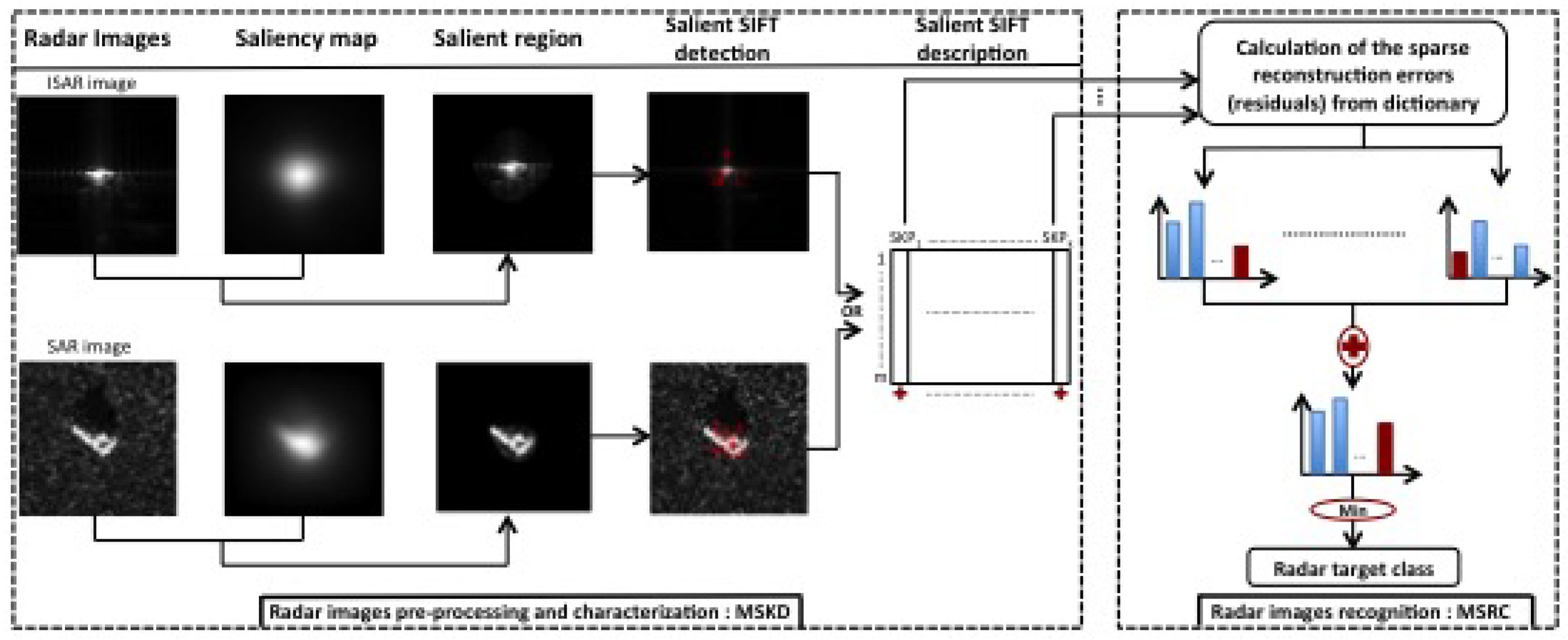
We illustrate in Figure 1 the working mechanism of the proposed method (MSKD-MSRC). It is composed by three complementary steps. The first and the second steps include the pre-processing and the characterization using MSKD method. The last step is dedicated to the recognition task using the MSRC classifier. These steps are detailed in the next subsections.
2.1. Radar Images Pre-Processing and Characterization: MSKD
As mentioned above, we combine the saliency map and SIFT descriptor in order to compute the MSKD for the radar images.
2.1.1. Saliency Attention
The human visual system (HVS) can automatically locate the salient regions on visual images. Inspired by the HVS mechanism, several saliency models are proposed to better understand how the attentional parts regions on images are selected. The most used model in the literature is that proposed by Itti et al. [9]. It locates well the salient regions on an image that visually attract the observers. To achieve this goal, this model exploits three channels: intensity, color and orientation. In this work, we do not integrate the color information using this model due to the grayscale nature of SAR and ISAR images. Based on the intensity channel, this model creates a Gaussian pyramid , where . To obtain the orientation channel from the intensity images, the model applies a pyramid of oriented Gabor filters , where is the orientation angles for each level of pyramid. After that, the feature maps (FM) of each channel are computed using the center-surround difference (⊖) between a center fine scale and a surround coarser scale as follows:
- Intensity:
- Orientation:
In total, 30 FM are generated (6 FM for intensity and 24 FM for orientation). To create one saliency map per channel, these feature maps are normalized and linearly combined. Finally, the overall saliency map is obtained by the summation of the two computed maps (intensity and orientation).
2.1.2. Scale Invariant Feature Transform (SIFT)
The scale invariant feature transform (SIFT) is a local method proposed by Lowe [20] to extract a set of descriptors from an image. This method has found a widespread use in different image processing applications [39,40,41]. The SIFT algorithm mainly covers four complementary steps:
- Scale space extrema detection: The image is transformed to a scale space by the convolution of the image with the Gaussian kernel :where is the standard deviation of the Gaussian probability distribution function.The difference of Gaussian (DOG) is computed as follows:where p is a factor to control the subtraction between two nearby scales. A pixel in the DOG scale space is considered as local extremum if it is the minimum or maximum of its 26 neighbors pixels (8 neighbors in the current scale and 9 neighbors in the adjacent scale separately).
- Unstable keypoints filtering: The found keypoints in the previous step are filtered to preserve the best candidates. Firstly, the algorithm rejects the keypoints with a DOG value less than a threshold, because these keypoints are with low contrast. Secondly, to discard the keypoints that are poorly localized along an edge, this algorithm uses a Hessian matrix :We note the ratio between the larger and the smaller eigenvalues of the matrix H. Then, the method eliminates the keypoints that satisfying:where is the trace and is the determinant.
- Orientation assignment: By selecting a region, we calculate the magnitude and the orientation of each keypoint. After that, a histogram of 36 bins weighted by a Gaussian and the gradient magnitude is built covering the 360 degree range of orientations. The orientation that achieves the peak of this histogram is assigned to the keypoint.
- Keypoint description: To generate the descriptor of each keypoint, we consider a neighboring region around the keypoint. This region has a size of pixels and are divided to 16 blocks of size pixels. For each block, a weighted gradient orientation histogram of 8 bins are computed. The descriptor is therefore composed by values.
2.1.3. Multi Salient Keypoints Descriptors (MSKD)
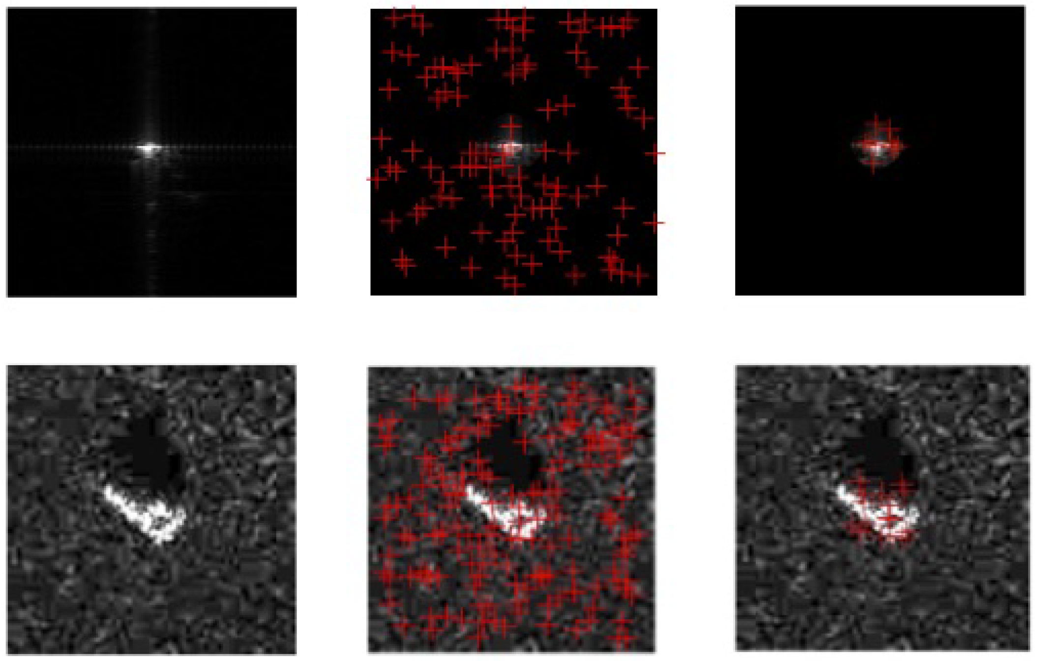
We illustrate in the second column of the Figure 2 the distribution of the SIFT applied to an example of ISAR and SAR images. It is clear that the SIFT generates a large number of keypoints to be processed. The majority of the these keypoints is located in the background of the radar images. This background does not present crucial information for radar image characterization. To handle this problem, we propose a new method called MSKD that combines saliency attention and SIFT methods. More precisely, we apply firstly the saliency attention model on the radar image. An example of the saliency maps of SAR and ISAR images are illustrated in the second column of Figure 1. It is observed that this model locates and enhances the most attractive regions of the input radar images which is the target area. This saliency map is exploited as a mask to segment the radar image into background and target areas. An example of this segmentation is illustrated in the third column of the Figure 1. From the segmented radar image, we compute the SIFT keypoints. In this way, we filter out the keypoints located in the background region as illustrated in the third column of Figure 2.
Finally, the descriptors matrix of one radar image is expressed as:
where k is the number of salient keypoints (SKP) in the radar image and m is the size of the descriptor of each SKP which is equal in our work to 128 values.
2.2. Radar Images Recognition: MSRC
After obtaining the MSKD for each test and training radar images, the next step consists of its classification using the MSRC. More specifically, we first construct a dictionary containing all MSKD of training radar images. Given the MSKD of the test radar image to classify, we solve an optimization problem that codes each descriptor (task) of the test radar image by a sparse vector. The l-2 norm difference between these sparse vectors and the descriptors leads to obtain the residuals (the error of the reconstruction) of each class for each MSKD. These residuals are after sum up. Finally, the class with the minimum residual is affected by the test radar image.
2.2.1. Dictionary Construction
The dictionary is obtained by the concatenation of all computed MSKD of training radar images as follows:
where s is the number of training radar images and n is the number of SKP in all training radar images.
2.2.2. Recognition via Multitask Sparse Framework
Given a radar image to recognize, we compute from it the set of local descriptors () using the MSKD method:
To recognize Y in sparse framework, we should compute the sparse reconstruction errors (residuals) for each task . After that, its class is found according to its sparse linear representation with all training samples:
with is the sparse coefficient matrix. To obtain it, the following optimization problem is solved as follows:
where and are respectively the -norm and the -norm, denotes the error tolerance. The Equation (11) represents a multitask problem since X and Y have multiple atoms (columns). This can be transformed to k -optimization problem, one for each (each task):
Equation (12) can be efficiently solved via second-order cone programming (SOCP) [42]. After obtaining the sparsest matrix , the total reconstruction error of each task for each class is computed as follows:
where is the labels of classes, represents the number of classes and is the characteristic function that selects only the coefficients associated with the c- class and set all others to be zero.
After that, the sum fusion is applied among all reconstruction residuals of all tasks according to the classes. Finally, the MSRC decides the class of the test sample as the class that produces the lowest total reconstruction error:
3. Experimental Results
In this section, we demonstrate the effectiveness of the proposed approach by conducting numerical recognition results on two radar images databases. The first one is composed of ISAR images and the second contains SAR images. To the best of our knowledge, until now there has not been a generic approach proposed in the literature that has the ability to recognize with the same treatment the ISAR and SAR images, excepting our previous work [18]. That is why aside from our MSKD-MSRC, we also implement three ATR methods which are practically close to the proposed method for a fair comparison. The first one uses the SIFT with matching (SIFT + matching). The second one consists of using the MSKD method in combination with the matching (MSKD + matching). The last one uses the SIFT descriptors as input of the MSRC (SIFT + MSRC). We note that the performance of the ATR system is related to its capabilities to locate the ROI containing the potential targets and its ability to provide a high recognition rate from the signature of the targets. We underline that all experiments are performed in the MATLAB 2016 environment with 3.10-GHz CPU Intel processor I5 and 24 GB of memory.
3.1. Experiment on ISAR Images
3.1.1. Database Description
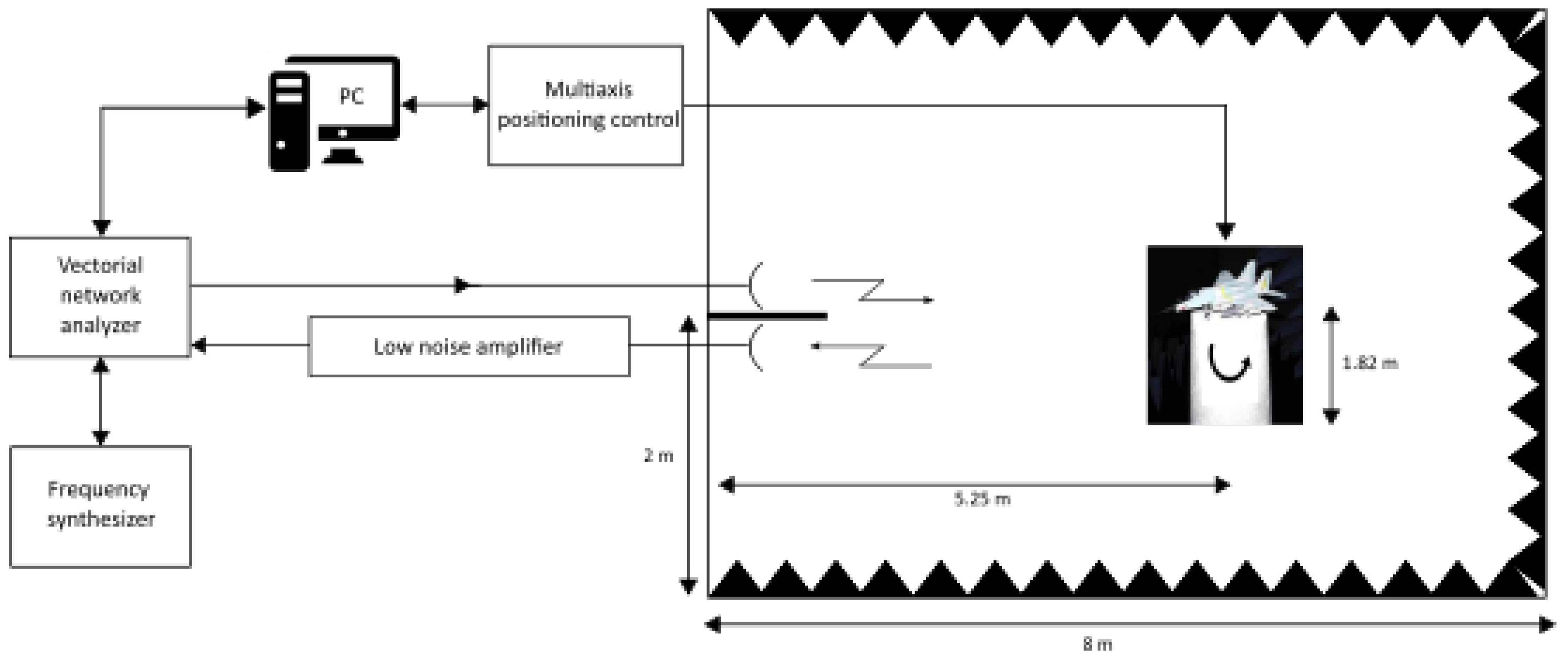
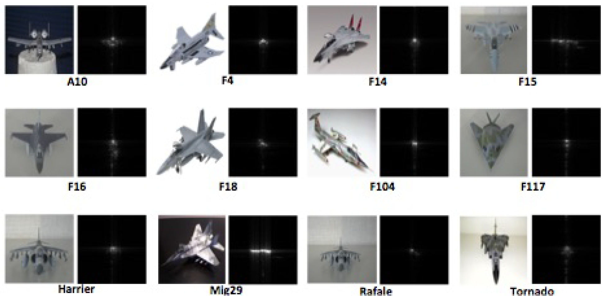
The ISAR images used in our work were acquired in the anechoic chamber of ENSTA Bretagne (Brest, France). The experimental setup of this chamber is depicted in Figure 3. The radar targets are illuminated with a frequency-stepped signal with a band varying between GHz and 18 GHz. A sequence of pulses is emitted using a frequency increment MHz. By applying the inverse fast Fourier transform (IFFT), we obtain 162 grayscale images per class with a size of pixels. To construct the ISAR database images, we have used 12 reduced aircraft models with reduced scale. For each target class, 162 ISAR images are generated. Consequently, the total number of ISAR images in this database is 1944. For rigorous details about the experiments conducted on the anechoic chamber, the reader is refereed to [1,43]. Samples of each aircraft target class of this dataset are displayed in Figure 4.
3.1.2. Target Recognition Results
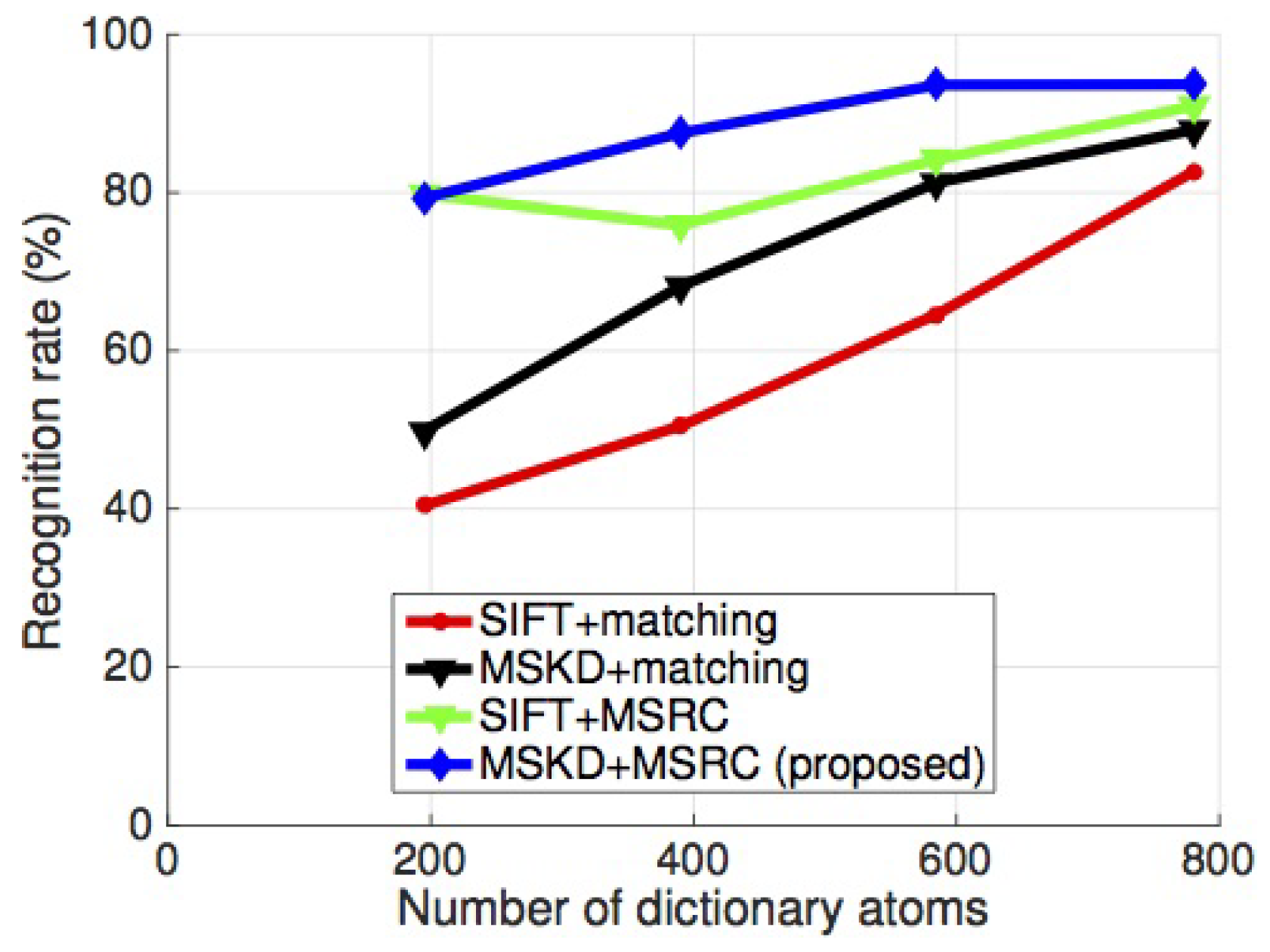
We study in Figure 5 the influence of the number of atoms in the dictionary (the size of training set) on the recognition rate. We select randomly 195, 390, 585 and 780 atoms that correspond to , , and of all ISAR images in the database respectively. The remaining ISAR images are used for the test. Consequently, we adopt configurations where the number of ISAR images in the training set are less than those of the test set. It is observed that all methods are sensitive to the number of dictionary atoms. When this number increases, the recognition rate rises as well. The proposed method outperforms the remaining ones under the different considered number of dictionary atoms. Additionally, comparing the matching and the MSRC to recognize the MSKD, it is observed that with the decreasing number of atoms, the recognition rate of MSKD + matching descends faster than that of the proposed method. In the upcoming experiments, we adopt 780 atoms. The comparison in terms of the overall recognition rate is given in Table 1 where those with the best accuracy are highlighted in bold. According to this table, some observations are concluded. First, the SIFT method combined with matching or MSRC provides the worst result. That is due to the location of keypoints in the background of the ISAR images which is not necessary for the recognition as illustrated in Figure 2. Conversely, the MSKD contributes to enhancing the recognition rate thanks to its concentration of SIFT keypoints in the target area. Then, by considering the matching or the MSKD, with a little number of keypoints of 23559 that corresponds to of the 420027 initial keypoints, the recognition rate is improved by and respectively. This issue demonstrates the benefit of the adopted filtration of the SIFT keypoints. Second, the MSRC performs better than the matching for SIFT and MSKD. That can be explained by the fact that the multitask sparsity of the MSKD of ISAR images leads to an enhancement of recognition rate.
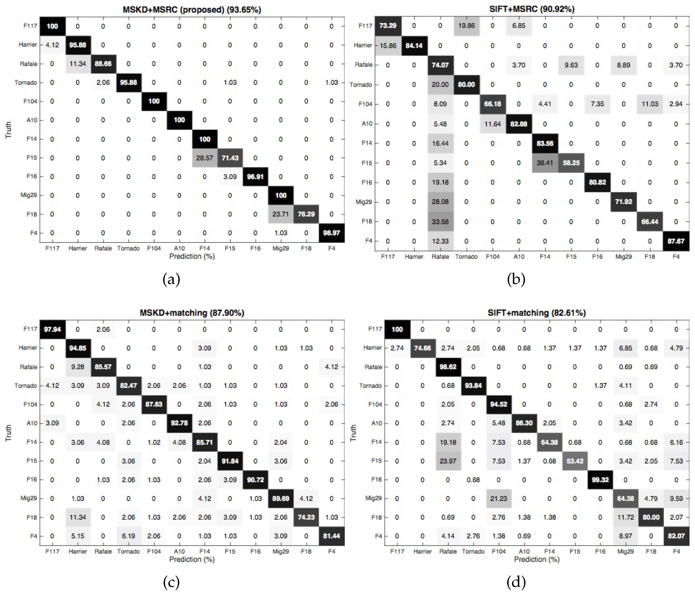
We provide in Figure 6 the confusion matrix of the proposed method as well as the remaining ones. For each confusion matrix, the diagonal values correspond to the recognition rate per class that should be high, while the rest of the values represent the misrecognition rate that must be low. The proposed method exceeds other methods for the recognition rate for all classes except for the F15 target. In addition, the MSKD + MSRC gives a recognition rate of for five target classes which are F117, F104, A10, F14 and Mig29. The SIFT + Matching gives a high recognition rate compared to other methods for only one class which is the Rafale. The overall recognition rate of the proposed method is which is , and better than SIFT + Matching, MSKD + matching and SIFT + MSRC methods respectively. This improvement demonstrates the power of the combination of the MSKD and the multitask sparse classifier to recognize the ISAR images.
3.1.3. Runtime Measurement
We study in this part the comparison of the runtime between the proposed method and three other methods. Table 2 records the mean runtime for pre-processing, feature extraction and recognition for each radar image in the database. We note that the mean runtime is computed by dividing the runtime of all ISAR images by the cardinal of the database. The sum of the runtime of these three steps gives the global mean runtime of each method. It is observed that the MSKD method is faster than the SIFT one for feature extraction. That is due to the small number of keypoints located using the MSKD. However, the pre-processing for the MSKD needs a remarkable runtime. For recognition, the matching or MSRC combined with the SIFT needs a heavy runtime compared with the MSKD. Moreover, the MSRC needs more runtime than matching. This is because of the time consumed by the optimized problem resolution for each task (each keypoint). Despite this issue, the MSRC significantly enhances the recognition rate. On the other hand, the SIFT + MSRC requires a computation time multiplied by compared to the proposed method.
3.2. Experiments on SAR Images
3.2.1. Databases Description
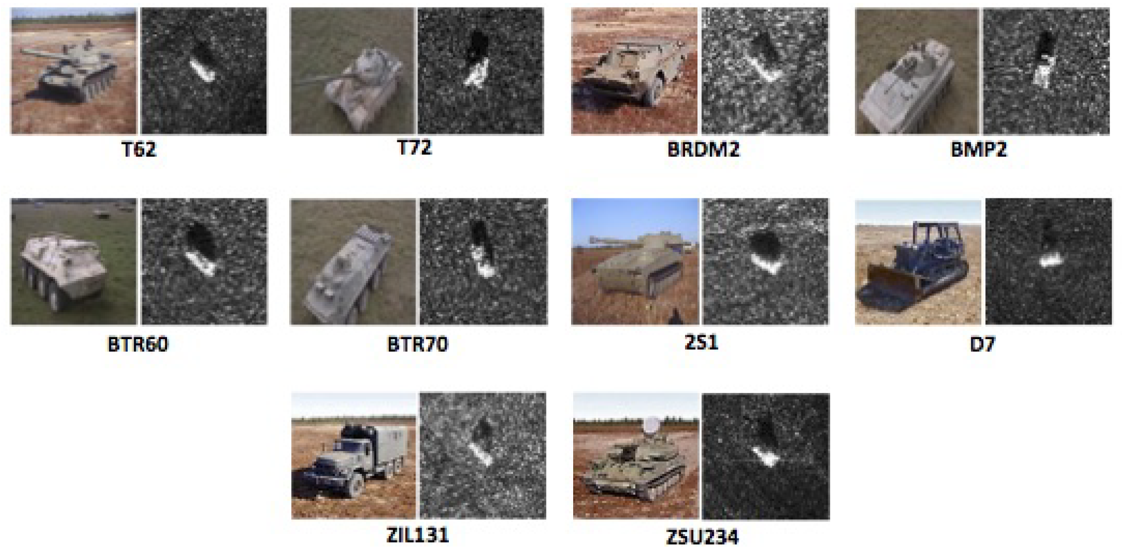
Regarding the SAR images, the moving and stationary target acquisition and recognition (MSTAR) public dataset (https://www.sdms.afrl.af.mil/index.php?collection=mstar) is used. This database is developed by Air Force Research Laboratory (AFRL) and the Defense Advanced Research Projects Agency (DARPA). The SAR images in this dataset are gathered by the X-band SAR sensor in spotlight mode. The MSTAR dataset includes multiple ground targets. Samples of each military ground target class of this dataset are displayed in Figure 7.
Two major versions are available for this dataset:
- SAR images under standard operating conditions (SOC, see Table 3). In this version, the training SAR images are obtained at the depression angle and the test ones at depression angle. Then, there is a depression angle difference of .
- SAR images under extended operating conditions (EOC) including:
- –
- The configuration variations (EOC-1, see Table 4). The configuration refers to small structural modifications and physical difference. Similarly to the SOC version, the training and the test targets are captured at and depressions angles respectively.
- –
- The depression variations (EOC-2, see Table 5). The SAR images acquired at depression angle are exploited for training, while the ones taken at , and depressions angles are used for testing.
The main difference between the SOC and EOC versions is that in the SOC, the condition of training and test sets are very near contrary to the EOC. We note that in the opposite case of the ISAR images database, the MSTAR is already partitioned to training and test datasets.
3.2.2. Target Recognition Results
We provide in Table 6 the quantitative comparison between the different methods on several versions of MSTAR dataset. As can be seen from this table, the MSKD performs much better than the use of the whole SIFT keypoints. This is because not all SIFT keypoints are useful to characterize the SAR images, and it can be remedied by the adopted filtration method as illustrated in Figure 2. This conclusion is an important motivation for coupling the saliency attention and the SIFT. Additionally, the use of the multitask SRC leads to an overwhelming superiority compared to the matching approach thanks to the sparse vectors extracted from each task in the SIFT and MSKD.
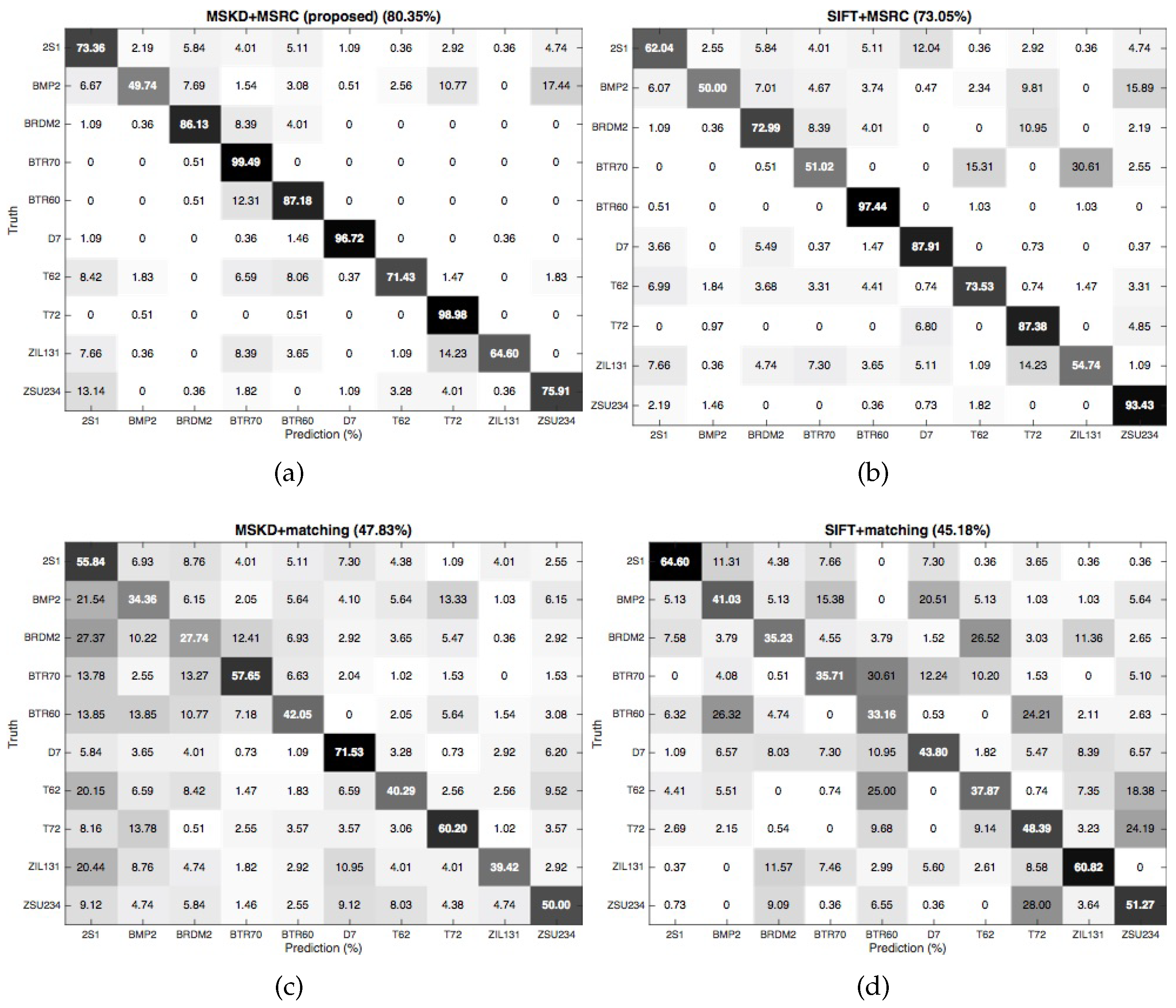
Considering the 10-class ground target (SOC), the recognition rate of the proposed method is which is , and better than the SIFT + matching, the MSKD + matching and the SIFT + MSRC. The SOC version of the MSTAR database is a big challenge due to its high number of existed SAR images. The confusion matrix of all methods are displayed in Figure 8. The proposed method provides a confusion between the BMP2, BRDM2 and BTR70 targets because they have the same vehicle type which is the armored personnel carriers. It is not able to correctly classify the BMP2 target. However, it has the high recognition rates for all classes compared to the remaining methods.
Regarding the configuration variations (EOC-1), the high recognition rate of is given by the proposed method compared to the remaining ones. It is an improvement of , and compared to the competitors. We give in Table 7 the confusion matrix of the different methods to be studied under EOC-1 version. We remark that the recognition rates of BMP2 and T72 are obviously less than BTR70 except the SIFT + MSRC method. This is because they have many variants included in the test set which do not exist in the training set. We note also that the MSKD-MSRC holds a remarkable superiority on BTR70 and T72 classes. However, it performs poorly on BMP2 class. Moreover, SIFT + Matching method is not able to recognize any images in the BTR70 class.
For the depression variations (EOC-2), the recognition rate is sharply degraded when the aspect angle increases for all methods. That is due to the variation between the aspect angles especially for and which represent a change of and compared to the train targets captured at . For instance, using the proposed method it drops from to to . The recognition rate of MSKD-MSRC still achieves the highest recognition rate in and depression angles. Whereas, the SIFT + Matching and the MSKD + matching work better for depression angle. Table 8 records the confusion matrix of all methods under EOC-2 using different depression angles. The proposed method gives a balanced recognition rate per class with a low value of the misclassification. However, for the depression angle, we show a high confusion between BRDM2 and 2S1 which drastically degrades the overall recognition rate. That is due to the large depression angle variance (from to ) between test and training SAR images. This issue modifies the global properties of SAR images, especially the ROI region, and consequently causes an abrupt change in the descriptors of the same target from different depression angles. Similarly, the depression angle enjoys the trend with a more moderate to depression angle.
3.2.3. Runtime Measurement
We record in the Table 9 a comparison between the execution time on different versions of the MSTAR database. Generally, the remarks presented in the Section 3.1.3 for ISAR images are also suitable for SAR images for MSTAR database. Additionally, the SIFT + MSRC requires more runtime than the proposed method. It is observed also that the SOC version needs a high runtime for MSRC. This is due to the large size of the dictionary (2747 atoms) that increases the time of the resolution of the optimization problem.
4. Discussion
The experiment results are obtained on two types of radar images which are ISAR (Section 3.1.1) and SAR images (Section 3.2.1). Lastly, different versions of MSTAR database (SOC, EOC1 and EOC2) are tested. We compared our method with three others. Several comparison criteria are used: the overall recognition rate, the recognition rate by class and the runtime. The objective of this contribution is to demonstrate that such an approach can be applied efficiently to SAR and ISAR images in the automatic radar target recognition problem.
Regarding the radar image characterization, the experiment results demonstrate that the proposed strategy enhances significantly the target recognition rates and speeds up the task of recognition. This is due to the pre-processing step that efficiently locates the ROI region through the saliency attention model. Consequently, the computation of the SIFT keypoints is faster than the use of the whole radar image. Additionally, the keypoints are concentrated in the salient region which increases the descriptor discrimination.
For the recognition stage, it is clear that the MSRC is slower than the matching but it contributes to increasing the recognition rate. On the other hand, the number of task used in the MSRC equals exactly to the number of keypoints. From that, the MSKD reduces the number of tasks and therefore accelerates the recognition step. We can conclude that the proposed method provides a trade-off between recognition rate and runtime.
Comparing both databases, the ISAR images provide the higher recognition rate. This is because the strong noise existed in the SAR images. In addition to this, the proposed method performs poorly for the high angles for the EOC-2 version of the MSTAR database. Generally, the difference in depression angles has more influence in recognition rate than the configuration variations. This issue is in compliance with the state-of-the-art results.
5. Conclusions and Future Work
This paper proposed a new generic algorithm called MSKD-MSRC for radar target recognition in ISAR/SAR images. Our approach represents each radar image with a set of salient keypoint descriptors (MKSD) located in the target area. For each test descriptor in the MSKD, a sparse reconstruction error (residual) according to each class is computed. After that, we sum all obtained residuals for the whole MSKD descriptors for all classes. The class with the minimum residual is affected to the test image. Extensive experiments are conducted on the ISAR images database and in the different versions of MSTAR dataset. Despite that, the SIFT and matching method performs worst for 10 classes (SOC) and 11 classes (ISAR images); it is a competitive method for three classes (EOC1 and EOC2). For all of the above performance comparisons in the experimental results, it can be concluded that despite that our approach does not provide the high recognition rate for all classes, it achieves in most cases the high overall recognition rates with a balanced performance for all ISAR and SAR classes in a reasonable runtime. Additionally, it effectively deals with the challenge of target recognition under EOC with a slight degradation for EOC-2 (). Considering the minor flaws of the proposed method, the future work will focus on using other local descriptors as well as testing the proposed system in other radar images databases such as those acquired in the maritime environment.
Author Contributions
Ayoub Karine proposed the general idea of the method presented and realized its application to real data. Abdelmalek Toumi, Ali Khenchaf and Mohammed El Hassouni, suggested the problematic and the field of application, reviewed the idea applied, and provided many suggestions. This manuscript was written globally by Ayoub Karine.
Conflicts of Interest
The authors declare no conflict of interest.
References
- Toumi, A.; Khenchaf, A.; Hoeltzener, B. A retrieval system from inverse synthetic aperture radar images: Application to radar target recognition. Inf. Sci. 2012, 196, 73–96. [Google Scholar] [CrossRef]
- El-Darymli, K.; Gill, E.W.; Mcguire, P.; Power, D.; Moloney, C. Automatic Target Recognition in Synthetic Aperture Radar Imagery: A State-of-the-Art Review. IEEE Access 2016, 4, 6014–6058. [Google Scholar] [CrossRef]
- Tait, P. Introduction to Radar Target Recognition; IET: Stevenage, UK, 2005; Volume 18. [Google Scholar]
- Toumi, A.; Hoeltzener, B.; Khenchaf, A. Hierarchical segmentation on ISAR image for target recongition. Int. J. Comput. Res. 2009, 5, 63–71. [Google Scholar]
- Bolourchi, P.; Demirel, H.; Uysal, S. Target recognition in SAR images using radial Chebyshev moments. Signal Image Video Process. 2017, 11, 1033–1040. [Google Scholar] [CrossRef]
- Ding, B.; Wen, G.; Ma, C.; Yang, X. Decision fusion based on physically relevant features for SAR ATR. IET Radar Sonar Navig. 2017, 11, 682–690. [Google Scholar] [CrossRef]
- Novak, L.M.; Benitz, G.R.; Owirka, G.J.; Bessette, L.A. ATR performance using enhanced resolution SAR. In Algorithms for Synthetic Aperture Radar Imagery III; International Society for Optics and Photonics: Orlanddo, FL, USA, 1996; Volume 2757, pp. 332–338. [Google Scholar]
- Chang, M.; You, X. Target Recognition in SAR Images Based on Information-Decoupled Representation. Remote Sens. 2018, 10, 138. [Google Scholar] [CrossRef]
- Itti, L.; Koch, C.; Niebur, E. A model of saliency-based visual attention for rapid scene analysis. IEEE Trans. Pattern Anal. Mach. Intell. 1998, 20, 1254–1259. [Google Scholar] [CrossRef]
- Kumar, N. Thresholding in salient object detection: A survey. In Multimedia Tools and Applications; Springer: Berlin, Germany, 2017. [Google Scholar]
- Borji, A.; Itti, L. State-of-the-Art in Visual Attention Modeling. IEEE Trans. Pattern Anal. Mach. Intell. 2013, 35, 185–207. [Google Scholar] [CrossRef] [PubMed]
- Gao, F.; You, J.; Wang, J.; Sun, J.; Yang, E.; Zhou, H. A novel target detection method for SAR images based on shadow proposal and saliency analysis. Neurocomputing 2017, 267, 220–231. [Google Scholar] [CrossRef]
- Wang, Z.; Du, L.; Zhang, P.; Li, L.; Wang, F.; Xu, S.; Su, H. Visual Attention-Based Target Detection and Discrimination for High-Resolution SAR Images in Complex Scenes. IEEE Trans. Geosci. Remote Sens. 2017, 56, 1855–1872. [Google Scholar] [CrossRef]
- Diao, W.; Sun, X.; Zheng, X.; Dou, F.; Wang, H.; Fu, K. Efficient Saliency-Based Object Detection in Remote Sensing Images Using Deep Belief Networks. IEEE Geosci. Remote Sens. Lett. 2016, 13, 137–141. [Google Scholar] [CrossRef]
- Song, H.; Ji, K.; Zhang, Y.; Xing, X.; Zou, H. Sparse Representation-Based SAR Image Target Classification on the 10-Class MSTAR Data Set. Appl. Sci. 2016, 6, 26. [Google Scholar] [CrossRef]
- Dong, G.; Kuang, G. A Soft Decision Rule for Sparse Signal Modeling via Dempster-Shafer Evidential Reasoning. IEEE Geosci. Remote Sens. Lett. 2016, 13, 1567–1571. [Google Scholar] [CrossRef]
- Dong, G.; Kuang, G.; Wang, N.; Zhao, L.; Lu, J. SAR Target Recognition via Joint Sparse Representation of Monogenic Signal. IEEE J. Sel. Top. Appl. Earth Obs. Remote Sens. 2015, 8, 3316–3328. [Google Scholar] [CrossRef]
- Karine, A.; Toumi, A.; Khenchaf, A.; Hassouni, M.E. Target Recognition in Radar Images Using Weighted Statistical Dictionary-Based Sparse Representation. IEEE Geosci. Remote Sens. Lett. 2017, 14, 2403–2407. [Google Scholar] [CrossRef]
- Clemente, C.; Pallotta, L.; Gaglione, D.; De Maio, A.; Soraghan, J.J. Automatic target recognition of military vehicles with Krawtchouk Moments. IEEE Trans. Aerosp. Electron. Syst. 2017, 53, 493–500. [Google Scholar] [CrossRef]
- Lowe, D. Distinctive Image Features from Scale-Invariant Keypoints. Int. J. Comput. Vis. 2004, 60, 91–110. [Google Scholar] [CrossRef]
- Zhu, X.; Ma, C.; Liu, B.; Cao, X. Target classification using SIFT sequence scale invariants. J. Syst. Eng. Electron. 2012, 23, 633–639. [Google Scholar] [CrossRef]
- Agrawal, A.; Mangalraj, P.; Bisherwal, M.A. Target detection in SAR images using SIFT. In Proceedings of the 2015 IEEE International Symposium on Signal Processing and Information Technology (ISSPIT), Abu Dhabi, UAE, 7–10 December 2015; pp. 90–94. [Google Scholar]
- Karine, A.; Toumi, A.; Khenchaf, A.; Hassouni, M.E. Target detection in SAR images using SIFT. In Proceedings of the 2017 IEEE International Conference on Advanced Technologies for Signal and Image Processing (ATSIP’2017), Fez, Morocco, 22–24 May 2017. [Google Scholar]
- Jdey, I.; Toumi, A.; Khenchaf, A.; Dhibi, M.; Bouhlel, M. Fuzzy fusion system for radar target recognition. Int. J. Comput. Appl. Inf. Technol. 2012, 1, 136–142. [Google Scholar]
- Sun, Y.; Liu, Z.; Todorovic, S.; Li, J. Adaptive boosting for SAR automatic target recognition. IEEE Trans. Aerospace Electron. Syst. 2007, 43, 112–125. [Google Scholar] [CrossRef]
- Huang, Z.; Pan, Z.; Lei, B. Transfer learning with deep convolutional neural network for SAR target classification with limited labeled data. Remote Sens. 2017, 9, 907. [Google Scholar] [CrossRef]
- El Housseini, A.; Toumi, A.; Khenchaf, A. Deep Learning for target recognition from SAR images. In Proceedings of the 2017 Seminar on Detection Systems Architectures and Technologies (DAT), Algiers, Algeria, 20–22 February 2017; pp. 1–5. [Google Scholar]
- Chen, S.; Wang, H.; Xu, F.; Jin, Y.Q. Target classification using the deep convolutional networks for SAR images. IEEE Trans. Geosci. Remote Sens. 2016, 54, 4806–4817. [Google Scholar] [CrossRef]
- Lin, Z.; Ji, K.; Kang, M.; Leng, X.; Zou, H. Deep convolutional highway unit network for sar target classification with limited labeled training data. IEEE Geosci. Remote Sens. Lett. 2017, 14, 1091–1095. [Google Scholar] [CrossRef]
- Wilmanski, M.; Kreucher, C.; Lauer, J. Modern approaches in deep learning for SAR ATR. In Algorithms for Synthetic Aperture Radar Imagery XXIII; International Society for Optics and Photonics: Baltimore, MD, USA, 2016; Volume 9843, p. 98430N. [Google Scholar]
- Wright, J.; Yang, A.Y.; Ganesh, A.; Sastry, S.S.; Ma, Y. Robust face recognition via sparse representation. IEEE Trans. Pattern Anal. Mach. Intell. 2009, 31, 210–227. [Google Scholar] [CrossRef] [PubMed]
- Li, W.; Du, Q. A survey on representation-based classification and detection in hyperspectral remote sensing imagery. Pattern Recognit. Lett. 2016, 83, 115–123. [Google Scholar] [CrossRef]
- Xing, X.; Ji, K.; Zou, H.; Chen, W.; Sun, J. Ship Classification in TerraSAR-X Images with Feature Space Based Sparse Representation. IEEE Geosci. Remote Sens. Lett. 2013, 10, 1562–1566. [Google Scholar] [CrossRef]
- Samadi, S.; Cetin, M.; Masnadi-Shirazi, M.A. Sparse representation-based synthetic aperture radar imaging. IET Radar Sonar Navig. 2011, 5, 182–193. [Google Scholar] [CrossRef] [Green Version]
- Yu, M.; Dong, G.; Fan, H.; Kuang, G. SAR Target Recognition via Local Sparse Representation of Multi-Manifold Regularized Low-Rank Approximation. Remote Sens. 2018, 10, 211. [Google Scholar]
- Wang, X.; Shao, Z.; Zhou, X.; Liu, J. A novel remote sensing image retrieval method based on visual salient point features. Sens. Rev. 2014, 34, 349–359. [Google Scholar] [CrossRef]
- Liao, S.; Jain, A.K.; Li, S.Z. Partial Face Recognition: Alignment-Free Approach. IEEE Trans. Pattern Anal. Mach. Intell. 2013, 35, 1193–1205. [Google Scholar] [CrossRef] [PubMed]
- Zhang, L.; Ding, Z.; Li, H.; Shen, Y.; Lu, J. 3D face recognition based on multiple keypoint descriptors and sparse representation. PLoS ONE 2014, 9, e100120. [Google Scholar] [CrossRef] [PubMed]
- Zhou, D.; Zeng, L.; Liang, J.; Zhang, K. Improved method for SAR image registration based on scale invariant feature transform. IET Radar Sonar Navig. 2017, 11, 579–585. [Google Scholar] [CrossRef]
- Bai, C.; Chen, J.N.; Huang, L.; Kpalma, K.; Chen, S. Saliency-based multi-feature modeling for semantic image retrieval. J. Vis. Commun. Image Represent. 2018, 50, 199–204. [Google Scholar] [CrossRef]
- Yuan, J.; Liu, X.; Hou, F.; Qin, H.; Hao, A. Hybrid-feature-guided lung nodule type classification on CT images. Comput. Gr. 2018, 70, 288–299. [Google Scholar] [CrossRef]
- Candes, E.; Romberg, J. l1-Magic: Rrrecovery of Sparse Signals via Convex Programming; Technical Report; California Institute of Technology: Pasadena, CA, USA, 2007. [Google Scholar]
- Bennani, Y.; Comblet, F.; Khenchaf, A. RCS of Complex Targets: Original Representation Validated by Measurements-Application to ISAR Imagery. IEEE Trans. Geosci. Remote Sens. 2012, 50, 3882–3891. [Google Scholar] [CrossRef]
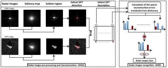
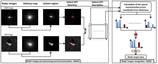
Figure 1.
Flowchart of the proposed ATR approach: MSKD-MSRC.

Figure 2.
SIFT and MSKD keypoints distribution. First column: ISAR and SAR images. Second column: SIFT keypoints distribution. Third column: MSKD keypoints distribution.
Figure 2.
SIFT and MSKD keypoints distribution. First column: ISAR and SAR images. Second column: SIFT keypoints distribution. Third column: MSKD keypoints distribution.

Figure 3.
Experimental setup of the anechoic chamber. Reproduced with permission from A. Toumi, Information sciences; published by ELSEVIER, 2012.
Figure 3.
Experimental setup of the anechoic chamber. Reproduced with permission from A. Toumi, Information sciences; published by ELSEVIER, 2012.

Figure 4.
Twelve classes of ISAR database.

Figure 5.
Recognition rate variation with the number of dictionary atoms on ISAR images database.

Figure 6.
Confusion matrix of the different methods on ISAR images database: (a) MSKD + MSRC; (b) SIFT + MSRC; (c) MSKD + matching; (d) SIFT + matching.
Figure 6.
Confusion matrix of the different methods on ISAR images database: (a) MSKD + MSRC; (b) SIFT + MSRC; (c) MSKD + matching; (d) SIFT + matching.

Figure 7.
Ten classes of MSTAR database: two tanks (T62 and T72), four armored personnel carriers (BRDM2, BMP2, BTR60 and BTR70), a rocket launcher (2S1), a bulldozer (D7), a truck (ZIL131), and an Air Defence Unit (ZSU234).
Figure 7.
Ten classes of MSTAR database: two tanks (T62 and T72), four armored personnel carriers (BRDM2, BMP2, BTR60 and BTR70), a rocket launcher (2S1), a bulldozer (D7), a truck (ZIL131), and an Air Defence Unit (ZSU234).

Figure 8.
Confusion matrix of the different methods on MSTAR dataset under SOC: (a) MSKD + MSRC; (b) SIFT + MSRC; (c) MSKD + matching; (d) SIFT + Matching.
Figure 8.
Confusion matrix of the different methods on MSTAR dataset under SOC: (a) MSKD + MSRC; (b) SIFT + MSRC; (c) MSKD + matching; (d) SIFT + Matching.


Table 1.
Comparison between the recognition rate (%) of different methods on ISAR images database.
| Methods | SIFT + Matching | MSKD + Matching | SIFT + MSRC | MSKD + MSRC (Proposed) |
|---|---|---|---|---|
| Recognition rate | 82.61 | 87.90 | 90.92 | 93.65 |
| Number of keypoints | 420,027 | 23,559 | 420,027 | 23,559 |
Table 2.
Comparison between the execution time (s) of different methods on ISAR images database.
| Methods | SIFT + Matching | MSKD + Matching | SIFT + MSRC | MSKD + MSRC (Proposed) |
|---|---|---|---|---|
| Pre-processing | 0 | 0.27 | 0 | 0.27 |
| Feature extraction | 0.24 | 0.08 | 0.24 | 0.08 |
| Recognition | 5.72 | 2.22 | 414.43 | 180.07 |
| Total | 5.96 | 2.57 | 414.67 | 180.42 |
Table 3.
Number of SAR images in MSTAR database under SOC.
| Target Classes | Depression Angle | |
|---|---|---|
| (Train) | (Test) | |
| T62 | 299 | 273 |
| T72 | 232 | 196 |
| BRDM2 | 298 | 274 |
| BMP2 | 233 | 195 |
| BTR60 | 256 | 195 |
| BTR70 | 233 | 196 |
| 2S1 | 299 | 274 |
| D7 | 299 | 274 |
| ZIL131 | 299 | 274 |
| ZSU234 | 299 | 274 |
| Total | 2747 | 2425 |
Table 4.
Number of SAR images in MSTAR database under configuration variation: EOC-1. The content in brackets represents the serial number of configuration.
Table 4.
Number of SAR images in MSTAR database under configuration variation: EOC-1. The content in brackets represents the serial number of configuration.
| Target Classes | Depression Angle | |
|---|---|---|
| BMP2 | 233 (snc21) | 196 (snc21) |
| 195 (snc9563) | ||
| 196 (snc9566) | ||
| BTR70 | 233 (c71) | 196 (c71) |
| 196 (snc132) | ||
| T72 | 233 (snc132) | 195 (sn812) |
| 191 (sn7) | ||
| Total | 689 | 1365 |
Table 5.
Number of SAR images in MSTAR database under depression variation: EOC-2.
| Target Classes | Depression Angle | |||
|---|---|---|---|---|
| Train | Test | |||
| 2S1 | 299 | 274 | 288 | 303 |
| BRDM2 | 298 | 274 | 420 | 423 |
| ZSU234 | 299 | 274 | 406 | 422 |
| Total | 896 | 822 | 1114 | 1148 |
Table 6.
Comparison between the recognition rate (%) of different methods on MSTAR dataset.
| Methods | SIFT + Matching | MSKD + Matching | ||
|---|---|---|---|---|
| Recognition Rate | Number of Keypoints | Recognition Rate | Number of Keypoints | |
| SOC | 45.18 | 183,963 | 47.83 | 35,459 |
| EOC-1 | 44.40 | 69,962 | 67.32 | 15,751 |
| EOC-2 () | 61.49 | 66,124 | 66.54 | 11,874 |
| EOC-2 () | 48.08 | 71,091 | 53.50 | 12,974 |
| EOC-2 () | 33.33 | 66,306 | 43.82 | 12,982 |
| SIFT + MSRC | MSKD + MSRC (proposed) | |||
| Recognition rate | Number of keypoints | Recognition rate | Number of keypoints | |
| SOC | 73.05 | 183,963 | 80.35 | 35,459 |
| EOC-1 | 70.84 | 69,962 | 84.54 | 15,751 |
| EOC-2 () | 70.63 | 66,124 | 84.18 | 11,874 |
| EOC-2 () | 49.42 | 71,091 | 68.58 | 12,974 |
| EOC-2 () | 37.34 | 66,306 | 36.32 | 12,982 |
Table 7.
Comparison between the confusion matrix (%) of different methods on MSTAR dataset under EOC-1 (configuration variation).
Table 7.
Comparison between the confusion matrix (%) of different methods on MSTAR dataset under EOC-1 (configuration variation).
| SIFT + Matching (44.40) | MSKD + Matching (67.32) | SIFT + MSRC (70.84) | |||||||
|---|---|---|---|---|---|---|---|---|---|
| BMP2 | BTR70 | T72 | BMP2 | BTR70 | T72 | BMP2 | BTR70 | T72 | |
| BMP2 | 80.58 | 0 | 19.42 | 52.98 | 5.96 | 41.06 | 82.15 | 10.36 | 7.49 |
| BTR70 | 53.57 | 0 | 46.42 | 10.20 | 82.14 | 7.65 | 17.28 | 60.13 | 22.59 |
| T72 | 77.14 | 0 | 22.85 | 20.27 | 2.92 | 76.80 | 12.06 | 17.69 | 70.25 |
| MSKD + MSRC (proposed) (84.54) | |||||||||
| BMP2 | BTR70 | T72 | |||||||
| BMP2 | 72.06 | 8.35 | 19.59 | ||||||
| BTR70 | 1.02 | 98.98 | 0 | ||||||
| T72 | 6.35 | 1.37 | 92.26 | ||||||
Table 8.
Comparison between the confusion matrix of different methods (%) on MSTAR dataset under EOC-2 (depression variation).
Table 8.
Comparison between the confusion matrix of different methods (%) on MSTAR dataset under EOC-2 (depression variation).
| SIFT + Matching (72.26) | MSKD + Matching (66.54) | SIFT + MSRC (70.63) | ||||||||
|---|---|---|---|---|---|---|---|---|---|---|
| 2S1 | BRDM2 | ZSU234 | 2S1 | BRDM2 | ZSU234 | 2S1 | BRDM2 | ZSU234 | ||
| 2S1 | 91.61 | 8.39 | 0 | 64.96 | 20.07 | 14.96 | 69.19 | 15.86 | 14.95 | |
| BRDM2 | 27.37 | 72.62 | 0 | 32.48 | 50 | 17.52 | 12.36 | 78.16 | 9.48 | |
| ZSU234 | 29.56 | 17.88 | 52.55 | 11.31 | 4.01 | 84.67 | 16.70 | 18.76 | 64.54 | |
| MSKD + MSRC (proposed) (84.18) | ||||||||||
| 2S1 | BRDM2 | ZSU234 | ||||||||
| 2S1 | 83.21 | 6.93 | 9.85 | |||||||
| BRDM2 | 7.66 | 91.97 | 0.36 | |||||||
| ZSU234 | 12.77 | 9.85 | 77.37 | |||||||
| SIFT + Matching (61.49) | MSKD + Matching (53.50) | SIFT + MSRC (49.42) | ||||||||
| 2S1 | BRDM2 | ZSU234 | 2S1 | BRDM2 | ZSU234 | 2S1 | BRDM2 | ZSU234 | ||
| 2S1 | 11.81 | 72.22 | 15.97 | 61.81 | 14.24 | 23.96 | 37.23 | 23.48 | 39.29 | |
| BRDM2 | 6.19 | 83.81 | 10 | 39.04 | 27.14 | 33.81 | 22.31 | 50.46 | 27.23 | |
| ZSU234 | 11.08 | 15.27 | 73.64 | 20.44 | 4.67 | 74.88 | 21.80 | 17.63 | 60.57 | |
| MSKD + MSRC (proposed) (68.58) | ||||||||||
| 2S1 | BRDM2 | ZSU234 | ||||||||
| 2S1 | 82.99 | 6.25 | 10.76 | |||||||
| BRDM2 | 42.85 | 33.81 | 23.33 | |||||||
| ZSU234 | 5.17 | 0.49 | 94.33 | |||||||
| SIFT + Matching (48.08) | MSKD + Matching (43.82) | SIFT + MSRC (37.34) | ||||||||
| 2S1 | BRDM2 | ZSU234 | 2S1 | BRDM2 | ZSU234 | 2S1 | BRDM2 | ZSU234 | ||
| 2S1 | 45.21 | 53.79 | 0.99 | 32.34 | 32.34 | 35.31 | 30.19 | 29.74 | 40.07 | |
| BRDM2 | 34.51 | 59.34 | 6.15 | 34.99 | 32.39 | 32.62 | 27.38 | 36.42 | 36.20 | |
| ZSU234 | 95.62 | 3.28 | 38 | 23.22 | 13.27 | 63.51 | 21.42 | 33.17 | 45.41 | |
| MSKD + MSRC (proposed) (36.32) | ||||||||||
| 2S1 | BRDM2 | ZSU234 | ||||||||
| 2S1 | 6.27 | 85.48 | 8.25 | |||||||
| BRDM2 | 39.24 | 35.46 | 25.30 | |||||||
| ZSU234 | 23.45 | 17.77 | 58.77 | |||||||
Table 9.
Comparison between the execution time (s) of different methods on MSTAR database.
| Methods | SIFT + Matching | MSKD + Matching | SIFT + MSRC | MSKD + MSRC (Proposed) | |
|---|---|---|---|---|---|
| Pre-processing | 0 | 0.08 | 0 | 0.08 | |
| Feature extraction | 0.02 | 0.009 | 0.02 | 0.09 | |
| SOC | Recognition | 76.87 | 2.46 | 933.21 | 780.34 |
| Total | 76.89 | 2.54 | 933.23 | 780.51 | |
| Pre-processing | 0 | 0.09 | 0 | 0.09 | |
| Feature extraction | 0.01 | 0.008 | 0.01 | 0.008 | |
| EOC-1 | Recognition | 3.14 | 0.72 | 57.69 | 30.01 |
| Total | 3.15 | 0.81 | 57.70 | 30.10 | |
| Pre-processing | 0 | 0.09 | 0 | 0.09 | |
| Feature extraction | 0.03 | 0.007 | 0.03 | 0.007 | |
| EOC-2 () | Recognition | 3.93 | 1.31 | 60.56 | 33.06 |
| Total | 3.96 | 1.40 | 60.59 | 33.15 | |
| Pre-processing | 0 | 0.06 | 0 | 0.06 | |
| Feature extraction | 0.01 | 0.003 | 0.01 | 0.003 | |
| EOC-2 () | Recognition | 4.13 | 1.30 | 60.07 | 34.35 |
| Total | 4.14 | 1.36 | 60.08 | 34.41 | |
| Pre-processing | 0 | 0.06 | 0 | 0.06 | |
| Feature extraction | 0.01 | 0.004 | 0.01 | 0.004 | |
| EOC-2 () | Recognition | 4.29 | 1.28 | 62.86 | 33.13 |
| Total | 4.30 | 1.34 | 62.87 | 33.19 |
© 2018 by the authors. Licensee MDPI, Basel, Switzerland. This article is an open access article distributed under the terms and conditions of the Creative Commons Attribution (CC BY) license (http://creativecommons.org/licenses/by/4.0/).
Share and Cite
MDPI and ACS Style
Karine, A.; Toumi, A.; Khenchaf, A.; El Hassouni, M. Radar Target Recognition Using Salient Keypoint Descriptors and Multitask Sparse Representation. Remote Sens. 2018, 10, 843. https://doi.org/10.3390/rs10060843
AMA Style
Karine A, Toumi A, Khenchaf A, El Hassouni M. Radar Target Recognition Using Salient Keypoint Descriptors and Multitask Sparse Representation. Remote Sensing. 2018; 10(6):843. https://doi.org/10.3390/rs10060843
Chicago/Turabian StyleKarine, Ayoub, Abdelmalek Toumi, Ali Khenchaf, and Mohammed El Hassouni. 2018. "Radar Target Recognition Using Salient Keypoint Descriptors and Multitask Sparse Representation" Remote Sensing 10, no. 6: 843. https://doi.org/10.3390/rs10060843
Note that from the first issue of 2016, this journal uses article numbers instead of page numbers. See further details here.