The Heterogeneity of Air Temperature in Urban Residential Neighborhoods and Its Relationship with the Surrounding Greenspace

Abstract

The thermal environment in residential areas is directly related to the living quality of residents. Therefore, it is important to understand thermal heterogeneity and ways to regulate temperature in residential neighborhoods. We investigated the spatial heterogeneity and temporal dynamics of air temperatures in 20 residential neighborhoods within the 5th ring road of Beijing, China. We further explored how the variations in air temperature were related to the patterns of the surrounding greenspace at different scales. We found that: (1) large air temperature differences existed among residential neighborhoods, with hourly maximum differences in air temperature reaching 5.30 °C on hot summer days; (2) not only the percentage but also the spatial configuration (e.g., edge density) of greenspace affected the local air temperature; and (3) the effects of spatial greenspace patterns on air temperature were scale dependent and varied by season. For example, increasing the proportion of greenspace in surrounding areas within a 100-m radius and increasing the edge density within radii from 500 to 1000 m could lower air temperatures in summer but not affect air temperatures in winter. In addition, decreasing the edge density of greenspaces within a 100-m radius of the surrounding areas would lead to an increase in air temperature in winter but not affect the air temperature in summer. These results extend our understanding of thermal environments and their relationships with greenspace patterns at the microscale (i.e., residential neighborhoods). They also provide useful information for urban planners to optimize greenspace patterns under better thermal conditions at the neighborhood scale.

1. Introduction

Urbanization has led to the phenomenon of urban heat islands (UHIs), which are defined by air temperatures in urban areas that are higher than those in the surrounding rural areas [1,2]. Numerous studies have examined the spatial patterns and temporal variations in UHI and related risk and mitigation strategies based on field observations, satellite data and modeling [3,4,5]. However, local cool islands also exist within urban areas, which are caused by different landscape patterns [6]. Urban residential areas are defined as areas where urban residents live and spend much of their time. Air temperatures in residential areas directly affect the health of urban dwellers and energy use [7,8,9]. Although simulations have been conducted to model temperature and evaluate how green and cool roofs can mitigate UHI effects in urban areas [10,11], few field observations have been conducted to reveal the spatial and temporal variations in air temperature in residential areas and their associations with residential landscape patterns.

With the availability of a dense meteorological network and mobile monitoring facilities, there is an increasing interest in measuring the intra-urban heterogeneity of air temperatures at fine scales [12,13,14]. These studies have reported that the maximum difference in air temperature could reach 9 °C in urban areas, and the differences are larger in summer [14,15]. These studies have also found that air temperatures vary by land use type. For example, central business districts are hotter than other land use types [12]. However, fewer studies have been conducted for residential areas [16].

Urban greenspaces (UGSs) can effectively mitigate the UHI effect [17,18,19,20,21,22]. UGSs reduce air temperatures mainly through two cooling functions: shading and evapotranspiration [23]. Shading reduces the input of solar radiation, while evapotranspiration converts sensible heat into latent heat [24,25]. Both the amount of UGSs and their spatial configuration affect these two cooling functions [20,26], which thereby affects the land surface temperature (LST) and air temperature [27,28]. A majority of previous studies have focused on how UGS patterns have affected LSTs [18,26,28,29], but few have focused on air temperatures [30,31,32,33,34]. This lack of studies is partially because LSTs can be directly derived from remotely sensed images, which provide spatially continuous data over large geographical extents. However, air temperature is more directly related to human comfort and health as opposed to LSTs and warrants more attention [7].

The overarching goal of this study is to understand the spatial variations and temporal dynamics of air temperatures in residential neighborhoods and examine how these variations in air temperature are related to spatial greenspace patterns in the surrounding areas at different scales. Specifically, we aim to: (1) quantify the spatial heterogeneity of air temperature and its temporal dynamics within residential areas; (2) explore the relationship between air temperature and pattern of UGSs, including percent cover and configuration of UGS; and (3) examine how these relationships vary by season and differ by scale. The results can expand our understanding of thermal environments in urban residential areas and provide useful insights for urban planners and designers on how to create a comfortable thermal microclimate by optimizing UGS patterns.

2. Materials and Methods

2.1. Study Area

Beijing is the capital of China and is located northeast of the North China Plain (longitude: 115°25′–117°30′E; latitude: 39°28′–41°25′N). It is located in a warm temperate zone and has a monsoon-influenced continental climate. The average daytime air temperature of Beijing ranges from 19 °C to 31 °C in summer and from −9 °C to 5 °C in winter. Studies have shown that the intensity of UHI effects has increased over the last several decades [35,36].

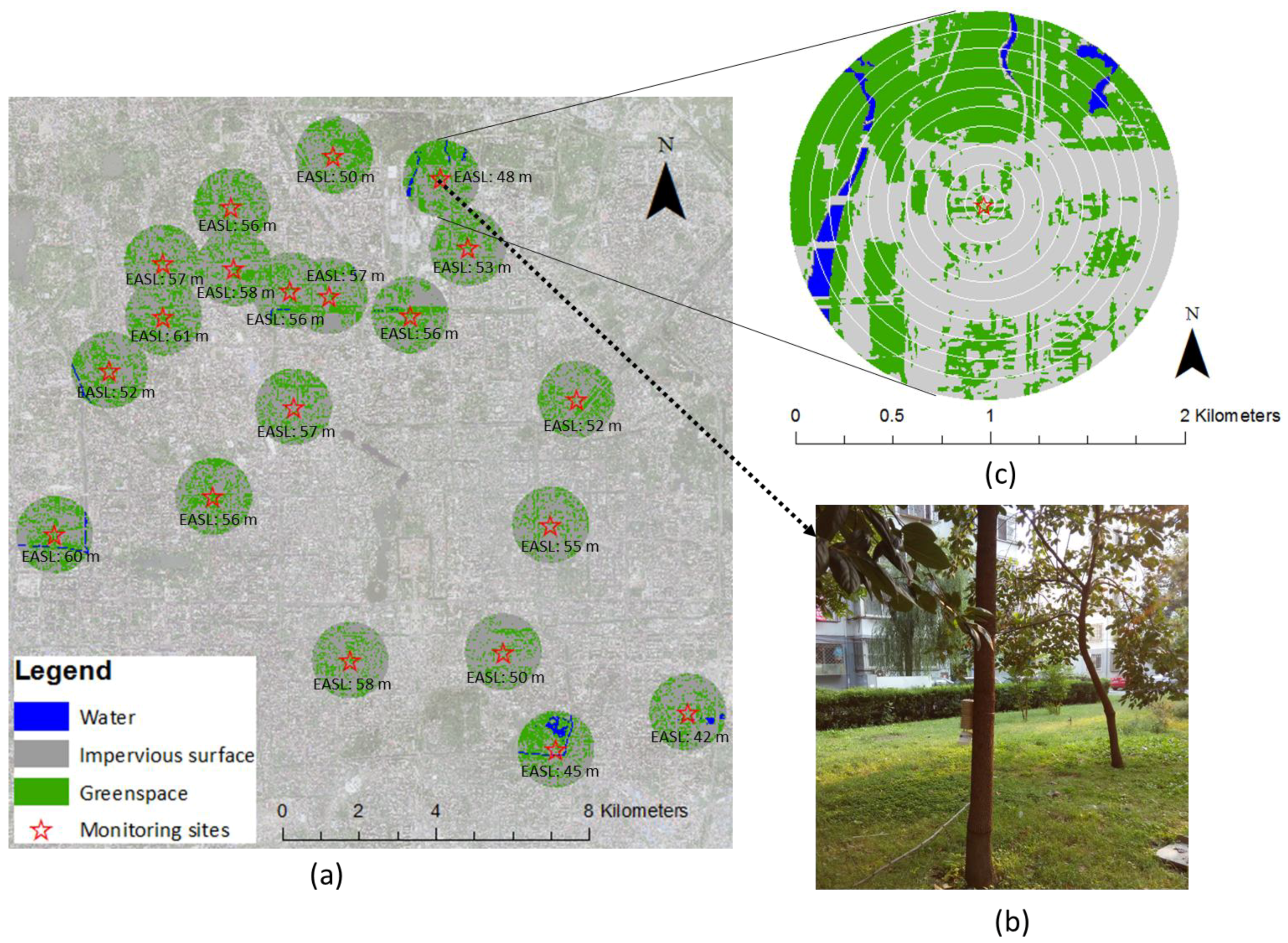
We chose 20 neighborhoods as the study sites (Figure 1a), and the areas around those sites (within a radius of 1 km) were used to study how UGSs influence air temperature. To minimize the influences caused by differences in elevation and anthropogenic heat, we chose neighborhoods that were located in highly developed areas, with elevations ranging from 41 m to 61 m (Figure 1a), and set the HOBO loggers at least 5-m away from the roads. Thus, these neighborhoods were ideal for studying the relationships between air temperature and the pattern of surrounding UGSs.

2.2. Classification of Land Cover for the Study Area

We used an image from Google Maps TM to map the land cover of the 20 neighborhoods and their surrounding areas (1-km radius). The date of acquisition for the satellite image from Google Maps TM was 11 July 2015. The image utilized 3 bands and had a spatial resolution of 0.5 m, which was sufficient for depicting fine-scale UGSs in urban residential areas. We identified three land cover types: UGSs (i.e., vegetation cover), impervious surfaces and water surfaces. The main component of the UGSs was trees, which had a small proportion of mixed shrubs and grasses. Impervious surfaces mainly consisted of roads and building roofs. Water was rare in and around the selected neighborhoods, and most of the water was in the park.

We mapped the land cover types using an object-based classification approach, which has been widely used to classify high-spatial-resolution images [37,38]. We classified the surrounding areas of each monitoring site within a 1-km radius. Specifically, we segmented the image into objects. Here, we used the multiresolution segmentation approach embedded in the commercial software Trimble eCognition. For multiresolution segmentation, the scale, shape and compactness parameters were customized to define the size and shape of the segmented objects. Based on the trial and error approach, we set the segmentation parameters of scale, color weight and compactness weight to 30, 0.9 and 0.5, respectively. Then, we conducted the classification using a support vector machine (SVM) as the classifier. We chose the radial basis function (RBF) kernel of the SVM, which has been proven to have good performance [39]. The RBF kernel has two parameters, cost (C) and gamma, which can affect the overall classification accuracy. We set parameters C and gamma for the SVM as 10⁶ and 10⁻⁵, respectively, as suggested in a previous study [38]. We randomly chose 200 training samples for each class for the supervised classification. We applied the most commonly used spectrum features in the classification (

Table 1. Object features used for classification.

Object Features	Description
Mean value a	Mean value of a specific band of an image object
Standard deviation a	Standard deviation of an image object
Brightness	Mean value of the 3 bands
Maximum difference	Maximum intensity difference of the 3 bands

^a Object features were calculated for each of the 3 bands.

). Finally, we applied a visual interpretation to improve the classification accuracy. After classification, we selected 100 random samples for each class to conduct an accuracy assessment. The final overall accuracy of the land cover map was 94.14%, and the kappa coefficient, which evaluates the consistency between the results and references, was 0.92. In addition, the user accuracy and product accuracy of the greenspace, which represent the commission and omission of the greenspace, were 96.51% and 95.40%, respectively.

2.3. Air Temperature Measurements

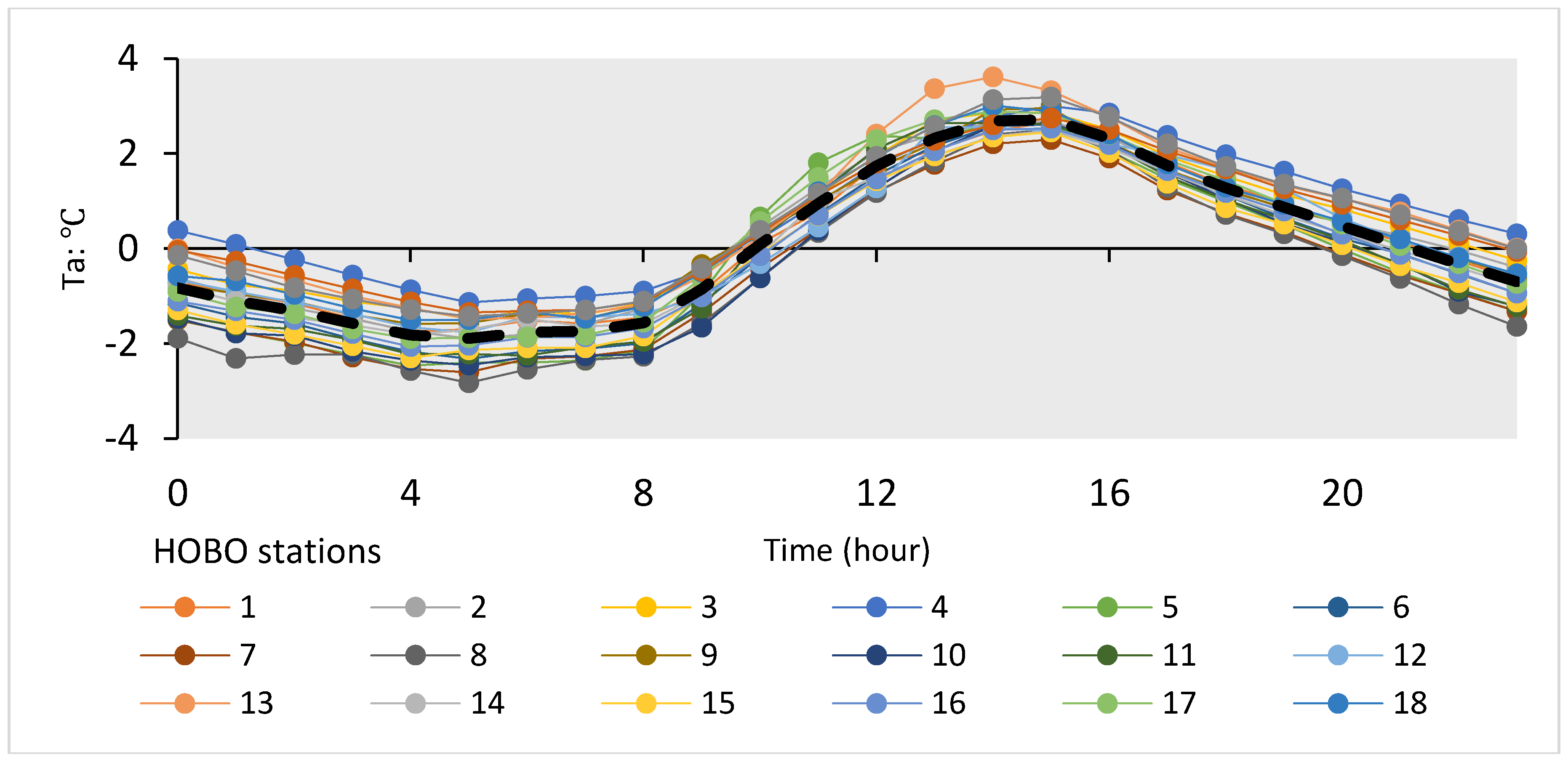
We used the HOBO U23 Pro v2 temperature/relative humidity data logger covered with a solar radiation shield to monitor air temperatures in the 20 neighborhoods. For each neighborhood, we selected one HOBO logger to represent the overall air temperature of the neighborhood. To make the monitoring results comparable, we set all HOBO loggers at the center of the UGS patches and kept them at least 5-m away from roads and public grounds to avoid human interruptions. All HOBO loggers were mounted on trees at a 1.5-m height (Figure 1b). We collected air temperatures from 17 August 2014 to 3 September 2014 in summer and from 1 December 2014 to 26 December 2014 in winter, with a sampling frequency of 10 min. By excluding days with rain, snow and extreme weather, we finally obtained 13 summer days and 15 winter days as the study period for the air temperature analysis.

2.4. Analysis of the Heterogeneity of Air Temperature in the Neighborhoods

We first plotted the daily variations in air temperature in the residential neighborhoods. Hourly air temperatures were calculated to analyze the differences and their dynamics. For each neighborhood, hourly temperatures were calculated in two steps. First, we summarized the mean temperature each hour; and, second, we averaged the hourly mean temperature for all summer days and winter days.

We then used two indicators to quantify the heterogeneity of the air temperature among the 20 neighborhoods during the day: the maximum difference in air temperature (MD) and the standard deviation of air temperature (SD). MD represents the air temperature difference between the hottest neighborhood and the coolest neighborhood. SD represents the standard deviation of the air temperature for all neighborhoods. MD represents the maximum heterogeneity, while SD represents the mean heterogeneity. Hourly MD and SD values were calculated to study the dynamics of air temperature differences among the neighborhoods.

In addition, we calculated the diurnal temperature range (DTR) for each neighborhood. The DTR represents the temperature difference between the highest temperature and lowest temperature during a given day. The DTR represents the variation in air temperature in a neighborhood. For each neighborhood, we first calculated the DTR for each day and averaged all DTRs for summer days and winter days for analysis.

2.5. Analysis of the Relationship between UGSs and Air Temperature

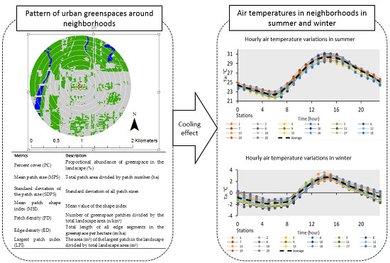
We used 13 circles with different radii around each monitoring site as the analytical units to evaluate the relationships between UGS and air temperature. These 13 circles were set with radii of 10 m, 20 m, 50 m, 100 m, 200 m, 300 m, 400 m, 500 m, 600 m, 700 m, 800 m, 900 m and 1000 m (Figure 1c). Within each unit, we calculated the percent cover (PC) and six other configuration metrics (i.e., mean patch size (MPS), standard deviation of the patch size (SDPS), patch density (PD), edge density (ED), mean shape index (MSI) and largest patch index (LPI)) of the UGS (

Table 2. Landscape metrics used in this study.

Metrics	Description	Equation
Percent cover (PC)	Proportional abundance of greenspace in the landscape (%)	$\frac{100}{A}\times {\displaystyle {\displaystyle \sum }_{i=1}^n}{a}_i$
Mean patch size (MPS)	Total patch area divided by patch number (ha)	$\frac{1}{10000\times n}\times {\displaystyle {\displaystyle \sum }_{i=1}^n}{a}_i$
Standard deviation of the patch size (SDPS)	Standard deviation of all patch sizes	$\sqrt{\frac{1}{n}\times {\displaystyle {\displaystyle \sum }_{i=1}^n}{\left(a_i-\overline{a}\right)}^2}$
Mean patch shape index (MSI)	Mean value of the shape index	$\frac{1}{n}\times {\displaystyle {\displaystyle \sum }_{i=1}^n}\frac{0.25\times e_i}{\sqrt{a_i}}$
Patch density (PD)	Number of greenspace patches divided by the total landscape area (n/km2)	$\frac{n}{A}\times {10}^6$
Edge density (ED)	Total length of all edge segments in the greenspace per hectare (m/ha)	$\frac{10000}{A}\times {\displaystyle {\displaystyle \sum }_{i=1}^n}{e}_i$
Largest patch index (LPI)	The area (m2) of the largest patch in the landscape divided by total landscape area (m2)	$\frac{\max \left(a_i\right)}{A}\times 100$

$a_i$ represents the area of patch i, $\overline{a}$ represents the average area of all patches, $e_i$ represents the length of the edge (or perimeter) of patch i, A represents the total area of the landscape, and n represents the total number of patches.

) that could potentially affect the air temperature [18,20,26,29]. For air temperature, we used the average temperature during summer and winter days. We first examined the Pearson correlation between air temperature and the seven metrics in each of the 13 units. Consequently, we calculated 91 Pearson coefficients in both summer and winter. To analyze the significance of these relationships at different scales, we explored effective radii for the effects of UGS on air temperature.

Because the configuration metrics are highly correlated with the proportion of greenspace, the Pearson correlation analysis may obtain spurious relationships between air temperature and the configuration metrics [26]. We further conducted a partial Pearson correlation analysis to investigate the relationships between air temperature and the configuration metrics after controlling the effects of the UGS proportion (i.e., using the PC as the controlled variable).

3. Results

3.1. Daily Variations in the Air Temperature of Residential Neighborhoods

The daily variations in the air temperature of the 20 neighborhoods were similar in both summer and winter (Figure 2 and Figure 3). Additionally, the daily variations recorded during summer and winter were also quite similar. From 0:00 to 6:00, the air temperatures in most neighborhoods continued decreasing; after 6:00, the temperatures started to increase, and they reached a maximum at 15:00. The temperatures then started to decrease until 24:00.

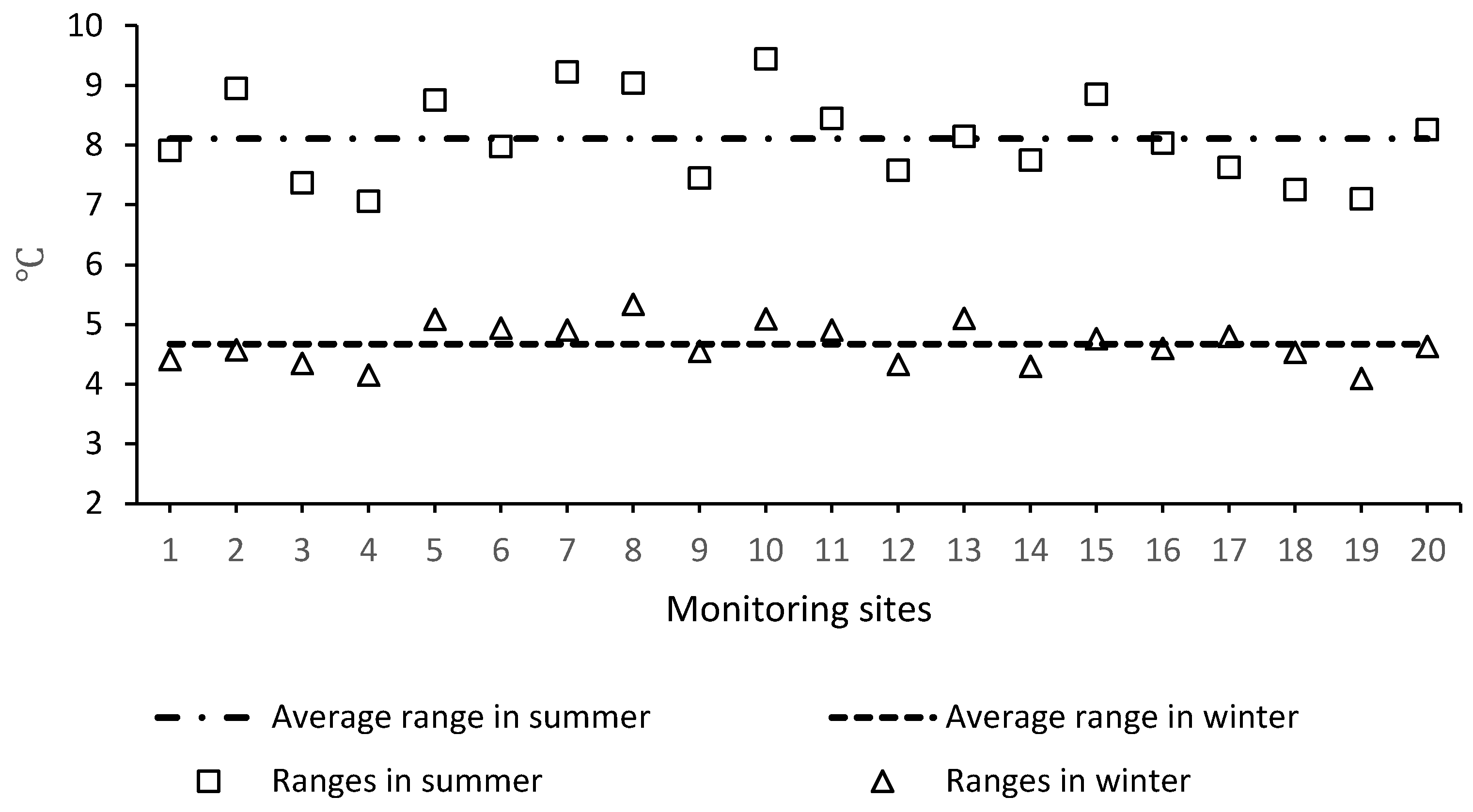
The DTR in summer was larger than that in winter (Figure 4). The DTRs in the 20 neighborhoods ranged from 7.1 to 9.4 °C in summer, with an average DTR of 8.1 °C. In winter, the DTRs ranged from 4.1 to 5.3 °C, with an average DTR of 4.6 °C. In addition, the variation in DTR among the 20 neighborhoods was larger in summer (2.3 °C) than in winter (1.2 °C).

3.2. The Heterogeneity of Air Temperature in Neighborhoods

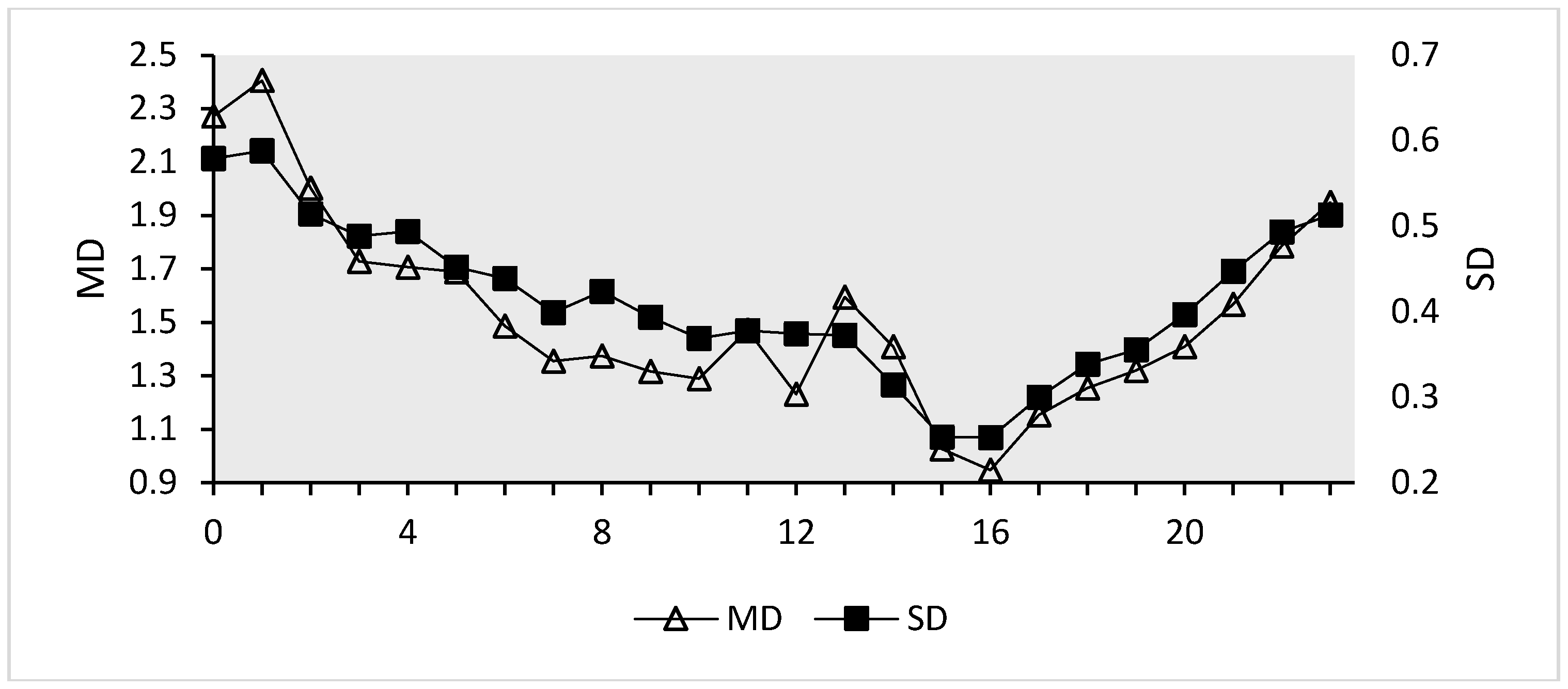
In both summer and winter, the variations in MD and SD were similar, which indicated that the largest heterogeneity and mean heterogeneity were consistent in residential areas. By comparing the variations in MD and SD in summer and winter, we found opposite tendencies. In summer, the MD and SD first increased and then decreased. In winter, the MD and SD decreased first and then increased (Figure 5 and Figure 6). In summer, from 0:00 to 14:00, the MD and SD increased from 1.02 to 1.90 °C and from 0.26 to 0.52 °C, respectively. From 14:00 to 24:00, the MD and SD decreased to 1.35 and 0.32 °C, respectively. In winter, from 0:00 to 16:00, the MD and SD decreased from 2.27 to 0.95 °C and from 0.58 to 0.25 °C, respectively. From 16:00 to 24:00, the MD and SD increased to 1.95 and 0.51 °C, respectively. In addition, the maximum air temperature differences in winter were larger than those in summer. In summer, the maximum MD and SD were 1.90 °C and 0.52 °C at 14:00, respectively, while, in winter, the maximum MD and SD were 2.40 °C and 0.59 °C at 1:00, respectively.

3.3. Relationship between Air Temperature and Its Surrounding UGSs

In summer, the PC of UGSs within radii of 20 m, 50 m and 100 m showed significantly negative correlations with air temperature (

Table 3. Pearson correlation between air temperature and landscape metrics in summer.

AU	PC	MPS	SDPS	MSI	PD	ED	LPI
10	−0.436	−0.484 * (R2 = 0.234)	0.166	0.270	0.166	−0.010	−0.436
20	−0.461 * (R2 = 0.213)	−0.228	−0.119	−0.070	−0.009	−0.141	−0.436
50	−0.624 ** (R2 = 0.389)	−0.070	−0.553 * (R2 = 0.306)	0.023	0.152	−0.177	−0.628 ** (R2 = 0.394)
100	−0.589 ** (R2 = 0.347)	−0.442	−0.489 * (R2 = 0.239)	−0.160	0.370	−0.249	−0.589 ** (R2 = 0.347)
200	−0.264	−0.326	−0.422	−0.250	0.158	−0.220	−0.414
300	−0.238	−0.288	−0.375	−0.236	0.170	−0.296	−0.344
400	−0.170	−0.165	−0.315	−0.263	0.152	−0.362	−0.346
500	−0.108	−0.150	−0.290	−0.305	0.133	−0.452 * (R2 = 0.204)	−0.351
600	−0.022	−0.057	−0.142	−0.260	0.080	−0.454 * (R2 = 0.206)	−0.226
700	0.009	−0.063	−0.069	−0.289	0.087	−0.515 * (R2 = 0.265)	−0.137
800	0.044	0.005	0.027	−0.242	0.051	−0.501 * (R2 = 0.251)	−0.044
900	0.059	0.009	0.076	−0.251	0.041	−0.513 * (R2 = 0.263)	0.007
1000	0.026	−0.011	0.077	−0.251	0.053	−0.516 * (R2 = 0.266)	0.030

* significant at the 0.05 level; ** significant at the 0.01 level. AU: analytical unit; PC: percent cover; MPS: mean patch size; SDPS: standard deviation of the patch size; MSI: mean shape index; PD: patch density; ED: edge density; LPI: largest patch index.

). The SDPS and LPI of the UGSs within radii of 50 m and 100 m showed significantly negative correlations with air temperature. The ED of the UGSs for radii from 500 to 1000 m showed significantly negative correlations with air temperature. The MPS within a radius of 20 m showed significantly negative correlations with air temperature. Other metrics showed no significant relationships with air temperature at any scale.

In winter, the PC of UGSs within radii of 200 m and between radii of 500 and 1000 m showed significantly negative correlations with air temperature (

Table 4. Pearson correlation coefficients between air temperature and landscape metrics in winter.

AU	PC	MPS	SDPS	MSI	PD	ED	LPI
10	−0.072	0.107	−0.405	−0.189	−0.405	−0.428	−0.071
20	−0.041	0.267	−0.428	0.113	−0.507 * (R2 = 0.257)	−0.527 * (R2 = 0.278)	−0.043
50	−0.087	0.219	0.137	0.378	−0.633 ** (R2 = 0.401)	−0.545 * (R2 = 0.297)	0.143
100	−0.342	0.066	−0.022	0.351	−0.428	−0.503 * (R2 = 0.253)	−0.057
200	−0.537 * (R2 = 0.288)	−0.058	−0.122	0.243	−0.305	−0.339	−0.192
300	−0.442	−0.013	−0.080	0.156	−0.364	−0.394	−0.149
400	−0.409	0.065	−0.070	0.240	−0.339	−0.336	−0.187
500	−0.450 * (R2 = 0.203)	0.051	−0.123	0.231	−0.331	−0.304	−0.259
600	−0.515 * (R2 = 0.265)	0.010	−0.139	0.268	−0.311	−0.278	−0.293
700	−0.507 * (R2 = 0.257)	0.006	−0.162	0.260	−0.318	−0.240	−0.283
800	−0.530 * (R2 = 0.281)	−0.007	−0.266	0.252	−0.321	−0.256	−0.438
900	−0.558 * (R2 = 0.311)	−0.013	−0.328	0.245	−0.331	−0.274	−0.444 * (R2 = 0.197)
1000	−0.534 * (R2 = 0.285)	0.002	−0.323	0.253	−0.342	−0.256	−0.451 * (R2 = 0.203)

* significant at the 0.05 level; ** significant at the 0.01 level. AU: analytical unit; PC: percent cover; MPS: mean patch size; SDPS: standard deviation of the patch size; MSI: mean shape index; PD: patch density; ED: edge density; LPI: largest patch index.

). The PD of the UGSs within radii of 20 m and 50 m was significantly negatively correlated with air temperature. The ED of UGSs within radii of 20 m, 50 m, and 100 m had significant negative relationships with air temperature. The LPI had negative correlations with air temperature with radii from 900 to 1000 m. Other metrics showed no significant relationships.

By comparing the impacts of seven metrics on air temperature in winter and summer, we found that the MSI showed no significant relationships with air temperature in both summer and winter; PC, ED and LPI affected air temperature in both seasons; and MPS and SDPS affected air temperature only in summer.

After controlling the effects of PC on UGSs, the relationship between air temperature and the configuration metrics changed greatly (

Table 5. Partial Pearson correlations between air temperature and the configuration metrics after controlling the effects of percent cover (PC) on UGS in summer.

AU	MPS	SDPS	MSI	PD	ED	LPI
10	−0.233	0.233	−0.050	0.233	0.126	−0.233
20	0.132	−0.156	−0.276	0.015	−0.071	0.439
50	0.332	−0.234	0.157	−0.015	0.149	−0.175
100	−0.130	−0.131	−0.160	0.329	0.085	−0.229
200	−0.231	−0.342	−0.268	0.162	−0.120	−0.338
300	−0.185	−0.303	−0.217	0.155	−0.197	−0.261
400	−0.078	−0.286	−0.245	0.143	−0.333	−0.372
500	−0.110	−0.314	−0.306	0.138	−0.481 * (R2 = 0.231)	−0.428
600	−0.053	−0.185	−0.261	0.080	−0.516 * (R2 = 0.266)	−0.314
700	−0.076	−0.113	−0.289	0.086	−0.600 ** (R2 = 0.360)	−0.211
800	−0.016	−0.012	−0.240	0.045	−0.609 ** (R2 = 0.371)	−0.119
900	−0.015	0.048	−0.247	0.031	−0.612 ** (R2 = 0.375)	−0.061
1000	−0.022	0.099	−0.250	0.049	−0.597 ** (R2 = 0.356)	0.016

* significant at the 0.05 level; ** significant at the 0.01 level. AU: analytical unit; PC: percent cover; MPS: mean patch size; SDPS: standard deviation of the patch size; MSI: mean shape index; PD: patch density; ED: edge density; LPI: largest patch index.

and

Table 6. Partial Pearson correlations between air temperature and the configuration metrics after controlling the effects of percent cover (PC) on UGS in winter.

AU	MPS	SDPS	MSI	PD	ED	LPI
10	0.396	−0.396	−0.335	−0.396	−0.408	0.396
20	0.406	−0.444	0.102	−0.504 * (R2 = 0.254)	−0.516 * (R2 = 0.266)	−0.045
50	0.313	0.269	0.406	−0.653 ** (R2 = 0.426)	−0.545 * (R2 = 0.297)	0.586 ** (R2 = 0.343)
100	0.332	0.284	0.382	−0.492 * (R2 = 0.242)	−0.340	0.361
200	0.272	0.272	0.269	−0.352	−0.117	0.308
300	0.359	0.348	0.253	−0.454	−0.170	0.322
400	0.441	0.373	0.335	−0.409	−0.138	0.286
500	0.395	0.336	0.257	−0.360	−0.107	0.143
600	0.371	0.387	0.294	−0.353	−0.075	0.107
700	0.327	0.363	0.276	−0.327	−0.051	0.102
800	0.310	0.282	0.255	−0.311	−0.064	−0.075
900	0.284	0.239	0.217	−0.299	−0.103	−0.033
1000	0.276	0.245	0.223	−0.308	−0.103	−0.058

* significant at the 0.05 level; ** significant at the 0.01 level. AU: analytical unit; PC: percent cover; MPS: mean patch size; SDPS: standard deviation of the patch size; MSI: mean shape index; PD: patch density; ED: edge density; LPI: largest patch index.

). In summer, the MPS, SDPS, and LPI were no longer significantly correlated with air temperature. However, ED still showed a significant relationship with air temperature within radii from 500 to 1000 m.

In winter, PD, ED, and LPI still showed significant relationships with air temperature but for different radii. PD showed a significant relationship with air temperature at radii of 20 m, 50 m and 100 m. ED had a significant relationship with air temperature at radii of 50 m and 100 m. LPI significantly affected air temperature at a radius of 50 m, which was quite different from the Pearson correlations.

4. Discussion

We found large differences in air temperature among residential neighborhoods. During the study period in summer, the average hourly MD reached 1.9 °C. On a hot day in summer, the hourly MD could reach 5.3 °C, which meant that the coolest neighborhood had an air temperature of only 30.6 °C but the hottest neighborhood could reach 36 °C; this value is above the warning temperature for China (35 °C) [40]. This difference has significant social and ecological implications. For example, when the daily mean air temperature reached 25 °C, the risk of daily death due to respiratory diseases largely increased in Beijing [7]. The large temperature difference also indicated that neighborhoods, particularly hotter neighborhoods, have the greatest potential for lower air temperatures in summer.

The dynamics of average air temperature differences among neighborhoods, which were represented by hourly MD and SD, were in accordance with temperature changes in summer, which indicated that solar radiation played a dominant role in air temperature differences in summer; thus, it is crucial to control the heating process (e.g., reduce solar radiation reaching the surface by implementing tree shading) to mitigate UHI effects in neighborhoods. In contrast, in winter, the dynamics of average air temperature differences were opposite those of temperature change, which indicated that anthropogenic heating (i.e., the main energy input at night) affected the air temperature. This pattern may be related to the heating supply for Beijing in winter.

Our results are consistent with previous studies in that the composition of UGSs could significantly affect in situ air temperatures [41]. Additionally, our results demonstrated that the configuration of UGSs also matters, especially regarding the ED of UGSs. The ED was negatively correlated with air temperature both in summer and winter at multiple scales, suggesting that increasing patch edges could significantly lower the air temperature because more edges likely reduce the solar radiation input by casting more shadows, which can thus decrease air temperatures. Because previous studies have mostly focused on the effects of the configuration on LSTs (e.g., [18,26]), our study enhanced the understanding of the cooling effects of UGSs on air temperature by adding evidence supporting the relationship between the ED and air temperature at different scales.

Our results further revealed that the effective radii at which the UGS patterns affected air temperature varied by season. In summer, the PC of UGSs in the immediate surrounding areas (within a radius of 100 m) significantly influenced air temperature, while, in winter, UGSs in much larger areas (radii larger than 500 m) affected temperature. Similarly, the effective radius at which the ED of UGSs affected air temperature also varied by season. In contrast to the PC of UGSs, in winter, the ED of UGSs in immediate surrounding areas significantly influenced air temperature, while, in summer, the ED of UGSs in much larger areas affected temperature. This characteristic is likely due to the weaker cooling functions, shading and evapotranspiration, of trees in winter because of the combination of lower temperatures, reduced solar radiation, and leaves falling off of trees. These results were different from a previous study that was conducted in Olympic Park, Beijing by Yan [41], where no seasonal effective scales were found in the relationship between the PC of UGSs and air temperature. However, this study only examined a maximum buffer of 300 m.

The differences in the effective radii of UGSs in summer and winter had important implications. Our results showed that UGSs lower air temperatures not only in summer but also in winter. While reducing air temperatures has positive effects in summer, it may have adverse impacts on energy use and human comfort in winter [42]. The differences in the effective radii of UGSs in summer and winter suggest that by changing the spatial pattern of UGSs at a certain radius, we can lower the air temperature in summer but not in winter. For example, increasing the PC of UGSs in surrounding areas within a 100-m radius and increasing the ED within radii from 500 to 1000 m could significantly lower air temperatures in summer but not significantly affect those in winter. Similarly, decreasing the ED of UGSs within a 100-m radius could increase air temperatures in winter but not affect those in summer.

This study has some limitations. First, the temperature sensors were set within relatively large UGS patches to avoid the interruption by human activities. Consequently, we found no significant relationship between air temperature and UGSs in the immediate surrounding areas (10-m radius), which was controversial in terms of understanding why UGSs closer to monitoring sites should have stronger impacts on the air temperature than those that are farther away. This result, however, is largely due to the percentage of UGSs within a 10-m radius, as all of the sites were similar (i.e., close to 100%), which did not contribute to the explanation of the variations in temperature. Second, this study did not fully explore the mechanisms behind the effects of UGS configuration on air temperature, which warrants more research in the future. Furthermore, we measured air temperature at a fixed point in each neighborhood, which may not fully represent the thermal conditions of the whole neighborhood. Future studies that consider the footprint of measured temperatures would be highly desirable [43,44,45].

5. Conclusions

Thermal environments in residential areas are directly related to the health and energy use of urban dwellers. We investigated the spatial patterns and temporal dynamics of the air temperature in residential neighborhoods and their relationships with the surrounding greenspace. This study compared the air temperature in residential neighborhoods within the 5th ring road of Beijing, China, in summer and winter. We further explored how these variations in air temperature were related to the spatial patterns of UGSs in surrounding areas by using different radii. The results showed that large differences in air temperature existed in different residential neighborhoods within a city. While some neighborhoods suffered from extreme heat, other neighborhoods had relatively comfortable thermal environments. Our results highlighted that not only the composition but also the configuration of greenspaces, especially the ED, influenced air temperatures. These results suggested that redesigning the spatial patterns of greenspaces within and near residential neighborhoods could effectively regulate air temperatures. The effective radius of greenspaces was different in summer and winter, which provided an opportunity to regulate air temperatures in one season while not affecting the air temperatures in the other season. We found that adding the percentage of greenspace within a radius of 100 m could significantly decrease the air temperature in summer without affecting the air temperature in winter. Decreasing the ED of a greenspace within 100 m and increasing the ED within radii from 500 to 1000 m could increase the local air temperature in winter while not decreasing the summer air temperature. The results of this study expanded our understanding of residential thermal environments and provided useful information for urban planners on how to decrease the air temperature in summer and increase the air temperature in winter by optimizing greenspace patterns within and near residential neighborhoods.

References

- Oke, T.R. The energetic basis of the urban heat island. Q. J. R. Meteorol. Soc. 1982, 108, 1–24. [Google Scholar] [CrossRef]
- Oke, T.R. City size and the urban heat island. Atmos. Environ. (1967) 1973, 7, 769–779. [Google Scholar] [CrossRef]
- Sharma, A.; Fernando, H.J.S.; Hamlet, A.F.; Hellmann, J.J.; Barlage, M.; Chen, F. Urban meteorological modeling using WRF: A sensitivity study. Int. J. Climatol. 2017, 37, 1885–1900. [Google Scholar] [CrossRef]
- Coffee, J.E.; Parzen, J.; Wagstaff, M.; Lewis, R.S. Preparing for a changing climate: The Chicago climate action plan’s adaptation strategy. J. Great Lakes Res. 2010, 36, 115–117. [Google Scholar] [CrossRef]
- Miao, S.; Chen, F.; Lemone, M.A.; Tewari, M.; Li, Q.; Wang, Y. An Observational and Modeling Study of Characteristics of Urban Heat Island and Boundary Layer Structures in Beijing. J. Appl. Meteorol. Climatol. 2009, 48, 484–501. [Google Scholar] [CrossRef]
- Stewart, I.; Oke, T. Newly developed “thermal climate zones” for defining and measuring urban heat island magnitidue in the canopy layer. In Proceedings of the Symposium & Eighth Symposium on Urban Environment, Phoenix, AZ, USA, 11–15 January 2009. [Google Scholar]
- Tao, H.; Tong, J.Y.; Shen, Y.H. Association between Daily Mean Air Temperature and Mortality of Respiratory Diseases in Beijing, China: A Case-Crossover Study. J. Environ. Health 2011, 9, 12–19. [Google Scholar]
- Kenney, W.L.; Craighead, D.H.; Alexander, L.M. Heat Waves, Aging, and Human Cardiovascular Health. Med. Sci. Sports Exerc. 2014, 46, 1891–1899. [Google Scholar] [CrossRef] [PubMed] [Green Version]
- Santamouris, M.; Papanikolaou, N.; Livada, I.; Koronakis, I.; Georgakis, C.; Argiriou, A.; Assimakopoulos, D. On the impact of urban climate on the energy consumption of buildings. Solar Energy 2001, 70, 201–216. [Google Scholar] [CrossRef]
- Sharma, A.; Conry, P.; Fernando, H.J.S.; Hamlet, A.F.; Hellmann, J.J.; Chen, F. Green and cool roofs to mitigate urban heat island effects in the Chicago metropolitan area: Evaluation with a regional climate model. Environ. Res. Lett. 2016, 11, 064004. [Google Scholar] [CrossRef]
- Li, D.; Bouzeid, E.; Oppenheimer, M. The effectiveness of cool and green roofs as urban heat island mitigation strategies. Environ. Res. Lett. 2014, in press. [Google Scholar] [CrossRef]
- Smoliak, B.V.; Snyder, P.K.; Twine, T.E.; Mykleby, P.M.; Hertel, W.F. Dense Network Observations of the Twin Cities Canopy-Layer Urban Heat Island*. J. Appl. Meteorol. Climatol. 2015, 54, 1899–1917. [Google Scholar] [CrossRef]
- Dobrovolný, P.; Krahula, L. The spatial variability of air temperature and nocturnal urban heat island intensity in the city of Brno, Czech Republic. Morav. Geogr. Rep. 2015, 23, 8–16. [Google Scholar] [CrossRef] [Green Version]
- Eliasson, I.; Svensson, M. Spatial air temperature variations and urban land use-a statistical approach. Meteorol. Appl. 2003, 10, 135–149. [Google Scholar] [CrossRef]
- Petralli, M.; Massetti, L.; Orlandini, S. Air temperature distribution in an urban park: Differences between open-field and below a canopy. In Proceedings of the 7th International Congress on Urban Climate, Yokohama, Japan, 29 June–3 July 2009. [Google Scholar]
- Hall, S.J.; Learned, J.; Ruddell, B.; Larson, K.L.; Cavender-Bares, J.; Bettez, N.; Groffman, P.M.; Grove, J.M.; Heffernan, J.B.; Hobbie, S.E. Convergence of microclimate in residential landscapes across diverse cities in the United States. Landsc. Ecol. 2016, 31, 101–117. [Google Scholar] [CrossRef]
- Kong, F.H.; Yin, H.W.; James, P.; Hutyra, L.R.; He, H.S. Effects of spatial pattern of greenspace on urban cooling in a large metropolitan area of eastern China. Landsc. Urban Plan. 2014, 128, 35–47. [Google Scholar] [CrossRef]
- Li, X.; Zhou, W.; Ouyang, Z.; Xu, W.; Zheng, H. Spatial pattern of greenspace affects land surface temperature: Evidence from the heavily urbanized Beijing metropolitan area, China. Landsc. Ecol. 2012, 27, 887–898. [Google Scholar] [CrossRef]
- Oliveira, S.; Andrade, H.; Vaz, T. The cooling effect of green spaces as a contribution to the mitigation of urban heat: A case study in Lisbon. Build. Environ. 2011, 46, 2186–2194. [Google Scholar] [CrossRef]
- Zhou, W.; Wang, J.; Cadenasso, M.L. Effects of the spatial configuration of trees on urban heat mitigation: A comparative study. Remote Sens. Environ. 2017, 195, 1–12. [Google Scholar] [CrossRef]
- Alves, E.D.L.; Lopes, A.M. The Urban Heat Island Effect and the Role of Vegetation to Address the Negative Impacts of Local Climate Changes in a Small Brazilian City. Atmosphere 2017, 8, 1–14. [Google Scholar]
- Jiao, M.; Zhou, W.; Zheng, Z.; Wang, J.; Qian, Y. Patch size of trees affects its cooling effectiveness: A perspective from shading and transpiration processes. Agric. For. Meteorol. 2017, 247, 293–299. [Google Scholar] [CrossRef]
- Bowler, D.E.; Buyung-Ali, L.; Knight, T.M.; Pullin, A.S. Urban greening to cool towns and cities: A systematic review of the empirical evidence. Landsc. Urban Plan. 2010, 97, 147–155. [Google Scholar] [CrossRef]
- Armson, D.; Stringer, P.; Ennos, A. The effect of tree shade and grass on surface and globe temperatures in an urban area. Urban For. Urban Green. 2012, 11, 245–255. [Google Scholar] [CrossRef]
- Akbari, H.; Pomerantz, M.; Taha, H. Cool surfaces and shade trees to reduce energy use and improve air quality in urban areas. Solar Energy 2001, 70, 295–310. [Google Scholar] [CrossRef]
- Zhou, W.; Huang, G.; Cadenasso, M.L. Does spatial configuration matter? Understanding the effects of land cover pattern on land surface temperature in urban landscapes. Landsc. Urban Plan. 2011, 102, 54–63. [Google Scholar] [CrossRef]
- Yan, H.; Dong, L. The impacts of land cover types on urban outdoor thermal environment: The case of Beijing, China. J. Environ. Health Sci. Eng. 2015, 13, 43. [Google Scholar] [CrossRef] [PubMed]
- Li, X.; Zhou, W.; Ouyang, Z. Relationship between land surface temperature and spatial pattern of greenspace: What are the effects of spatial resolution? Landsc. Urban Plan. 2013, 114, 1–8. [Google Scholar] [CrossRef]
- Peng, J.; Xie, P.; Liu, Y.; Ma, J. Urban thermal environment dynamics and associated landscape pattern factors: A case study in the Beijing metropolitan region. Remote Sens. Environ. 2016, 173, 145–155. [Google Scholar] [CrossRef]
- Upmanis, H.; Eliasson, I.; Lindqvist, S. The influence of green areas on nocturnal temperatures in a high latitude city (Göteborg, Sweden). Int. J. Climatol. 1998, 18, 681–700. [Google Scholar] [CrossRef] [Green Version]
- Monteiro, M.V.; Doick, K.J.; Handley, P.; Peace, A. The impact of greenspace size on the extent of local nocturnal air temperature cooling in London. Urban For. Urban Green. 2016, 16, 160–169. [Google Scholar] [CrossRef]
- Doick, K.J.; Peace, A.; Hutchings, T.R. The role of one large greenspace in mitigating London’s nocturnal urban heat island. Sci. Total Environ. 2014, 493C, 662–671. [Google Scholar] [CrossRef] [PubMed]
- Chang, C.-R.; Li, M.-H.; Chang, S.-D. A preliminary study on the local cool-island intensity of Taipei city parks. Landsc. Urban Plan. 2007, 80, 386–395. [Google Scholar] [CrossRef]
- Von Stülpnagel, A.; Horbert, M.; Sukopp, H. The importance of vegetation for the urban climate. In Urban Ecology. Plants and Plant Communities in Urban Environments; SPB Academic Publication: The Hague, The Netherlands, 1990; pp. 175–193. [Google Scholar]
- Liu, Y.; Xu, Y.; Ma, J.; Quan, W. Quantitative Assessment and Planning Simulation of Beijing Urban Heat Island. Ecol. Environ. Sci. 2014, 23, 1156–1163. [Google Scholar]
- Hu, X.; Zhou, W.; Qian, Y.; Yu, W. Urban expansion and local land-cover change both significantly contribute to urban warming, but their relative importance changes over time. Landsc. Ecol. 2016, 32, 1–18. [Google Scholar] [CrossRef]
- Blaschke, T. Object based image analysis for remote sensing. Isprs J. Photogramm. Remote Sens. 2010, 65, 2–16. [Google Scholar] [CrossRef]
- Qian, Y.; Zhou, W.; Yan, J.; Li, W.; Han, L. Comparing Machine Learning Classifiers for Object-Based Land Cover Classification Using Very High Resolution Imagery. Remote Sens. 2015, 7, 153–168. [Google Scholar] [CrossRef]
- Kavzoglu, T.; Colkesen, I. A kernel functions analysis for support vector machines for land cover classification. Int. J. Appl. Earth Observ. Geoinform. 2009, 11, 352–359. [Google Scholar] [CrossRef]
- Xu, X.; Zheng, Y.; Yin, J.; Wu, R. Characteristics of high temperature and heat wave in Nanjing City and their impacts on human health. Chin. J. Ecol. 2011, 30, 2815–2820. [Google Scholar]
- Yan, H.; Fan, S.; Guo, C.; Hu, J.; Dong, L. Quantifying the Impact of Land Cover Composition on Intra-Urban Air Temperature Variations at a Mid-Latitude City. PLoS ONE 2014, 9, e102124. [Google Scholar] [CrossRef] [PubMed]
- Anderson, B.G.; Bell, M.L. Weather-related mortality: How heat, cold, and heat waves affect mortality in the United States. Epidemiology 2009, 20, 205. [Google Scholar] [CrossRef] [PubMed]
- Grimmond, C.S.B. Progress in measuring and observing the urban atmosphere. Theor. Appl. Climatol. 2006, 84, 3–22. [Google Scholar] [CrossRef]
- Oke, T.R. Initial guidance to obtain representative meteorological observations at urban sites. Available online: https://www.researchgate.net/publication/265347633_Initial_guidance_to_obtain_representative_meteorological_observations_at_urban_sites (accessed on 15 June 2018).
- Alves, E.D.L.; Biudes, M.S. Method for determining the footprint area of air temperature and relative humidity. Acta Scientiarum Technol. 2013, 35, 187–194. [Google Scholar] [CrossRef]
Figure 1.
Study area showing the: (a) spatial distribution of the 20 residential neighborhoods, with an elevation above sea level (EASL) ranging from 41 to 61 m, and the corresponding land cover map; (b) field air temperature measurements using HOBO loggers covered by solar radiation shields; and (c) circles with different radii around the monitoring sites.
Figure 2.
Hourly air temperature variations over 20 neighborhoods in summer.
Figure 3.
Hourly air temperature variations over the 20 neighborhoods in winter.
Figure 4.
Diurnal temperature ranges (DTRs) for air temperature in the 20 neighborhoods.
Figure 5.
The hourly maximum differences in air temperature (MD) and the hourly standard deviation of air temperature (SD) in summer.
Figure 6.
The hourly maximum differences in air temperature (MD) and the hourly standard deviation of air temperature (SD) in winter.