Detecting and Quantifying a Massive Invasion of Floating Aquatic Plants in the Río de la Plata Turbid Waters Using High Spatial Resolution Ocean Color Imagery


Abstract
:
1. Introduction
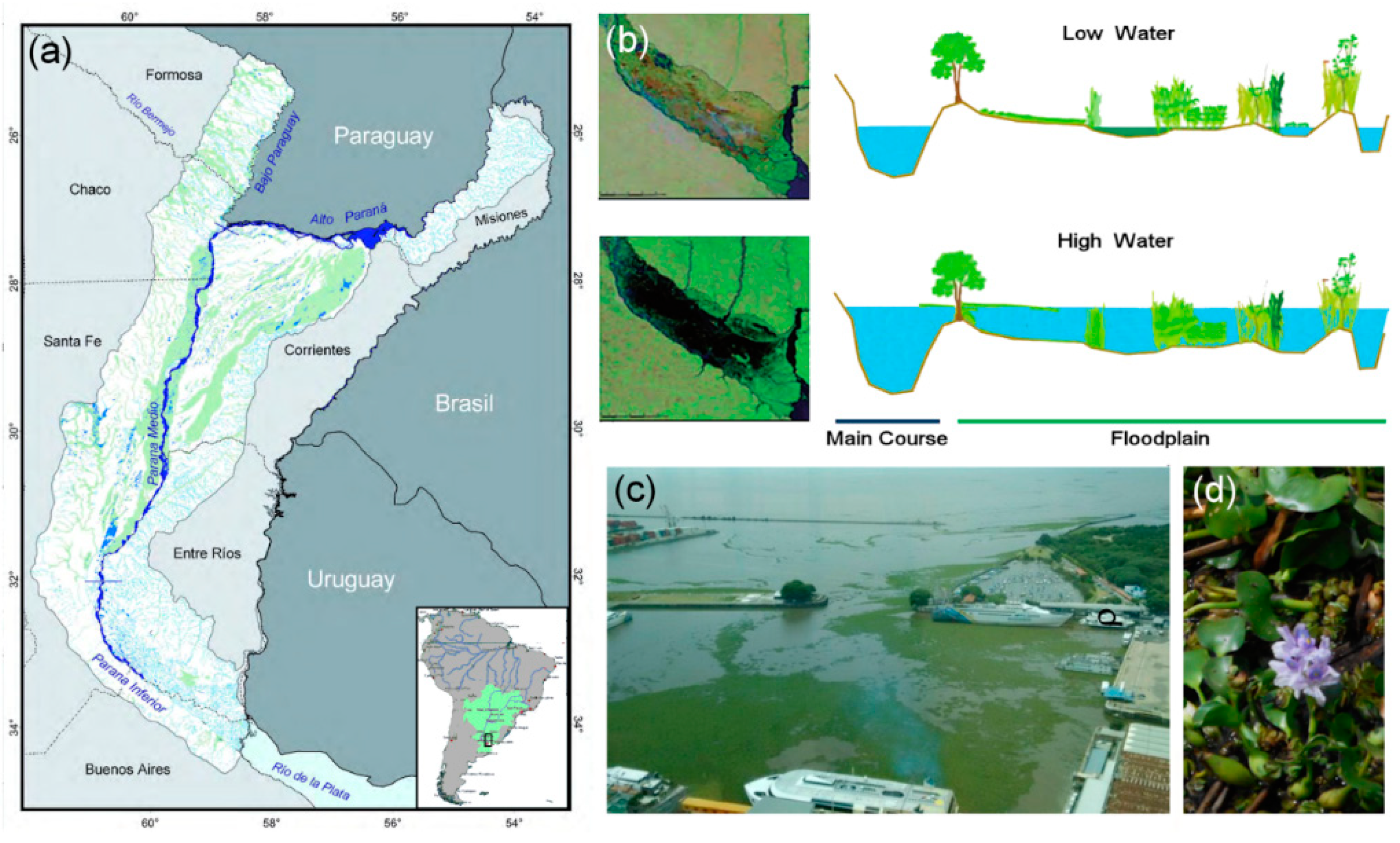
2. Study Area
3. Materials and Methods
3.1. Satellite Data
3.2. Field Data
4. Results and Discussion
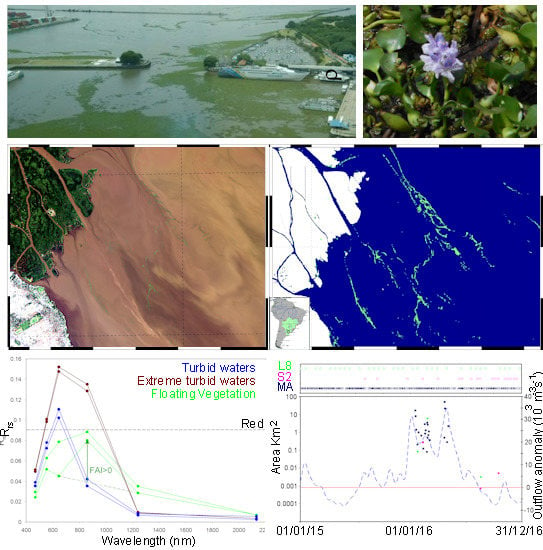
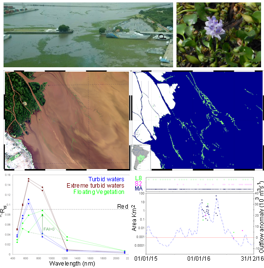
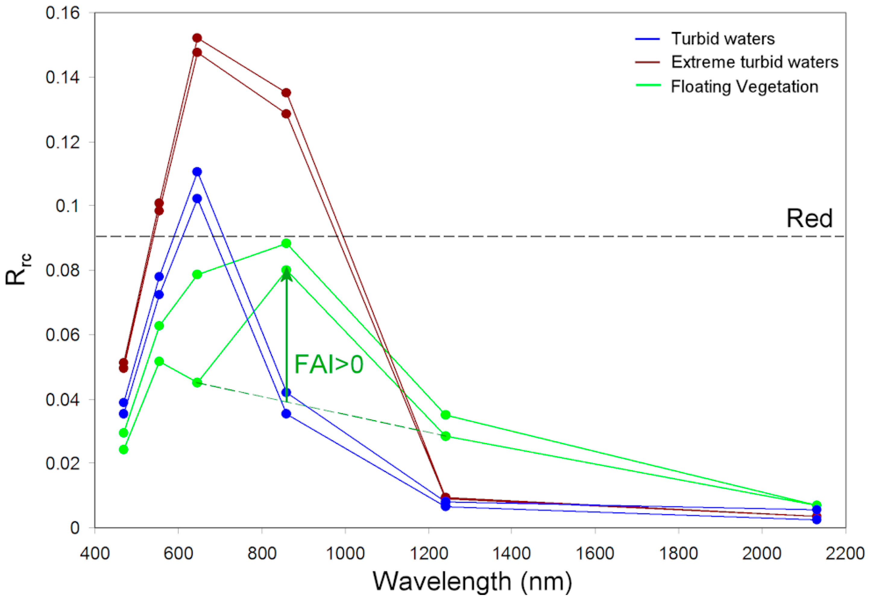
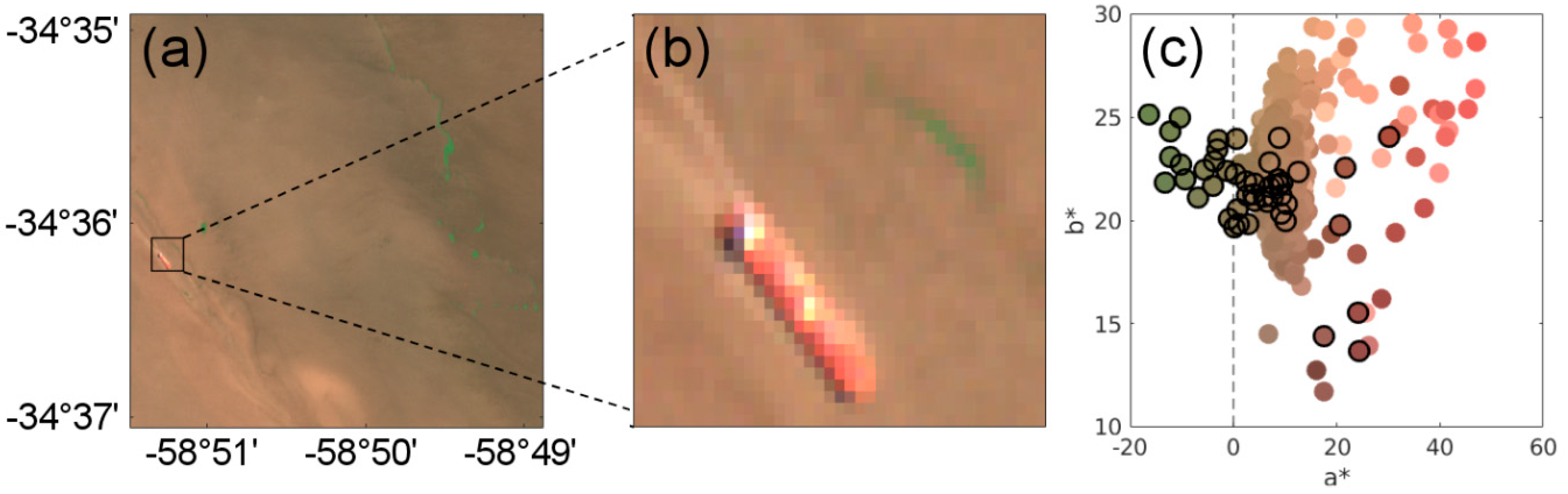
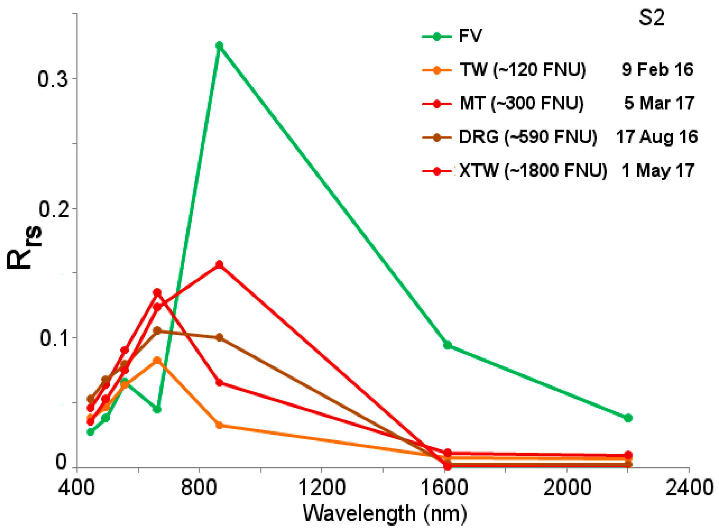
4.1. Spectral Features of Eichhornia Crassipes
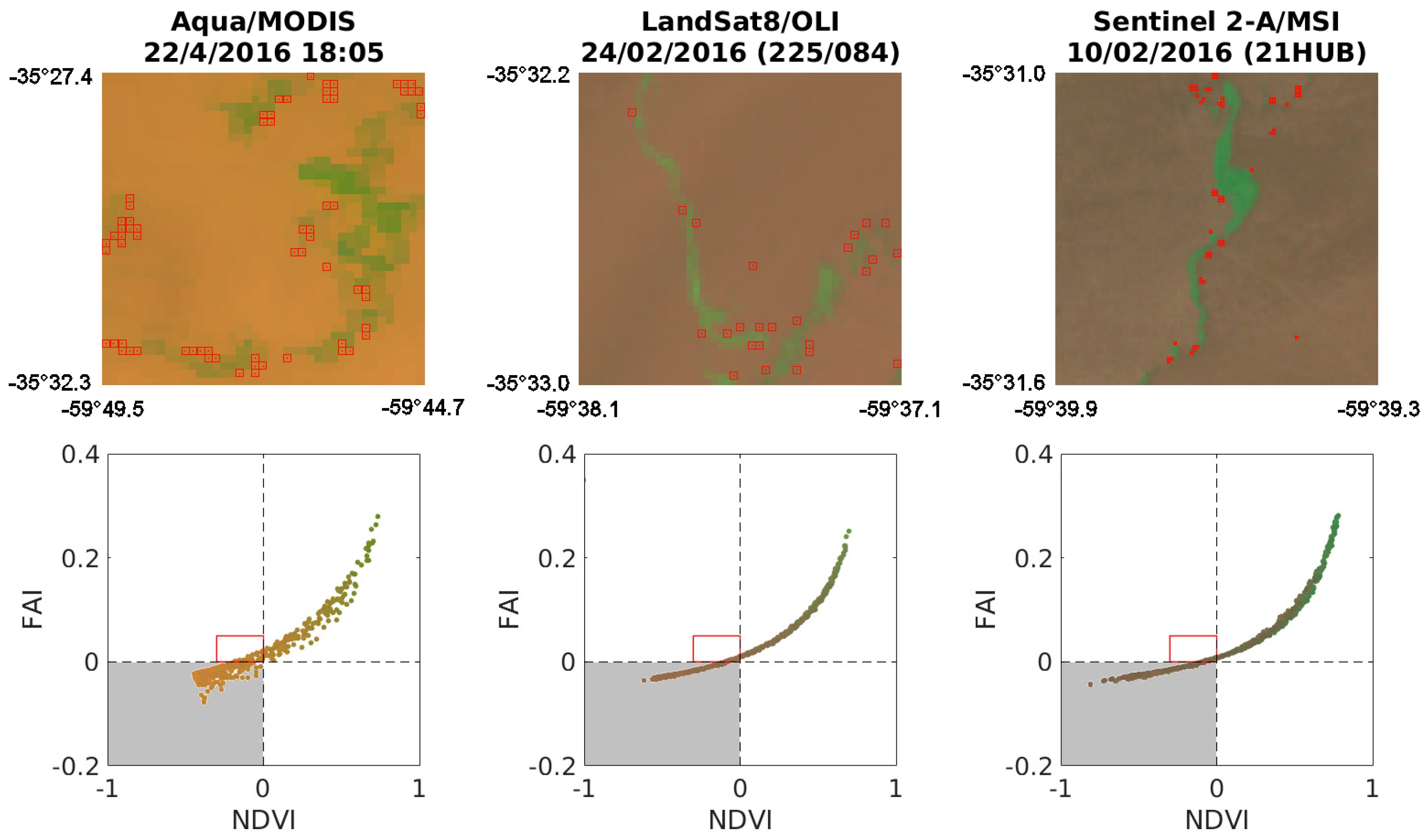
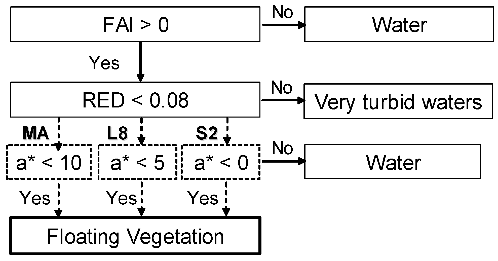
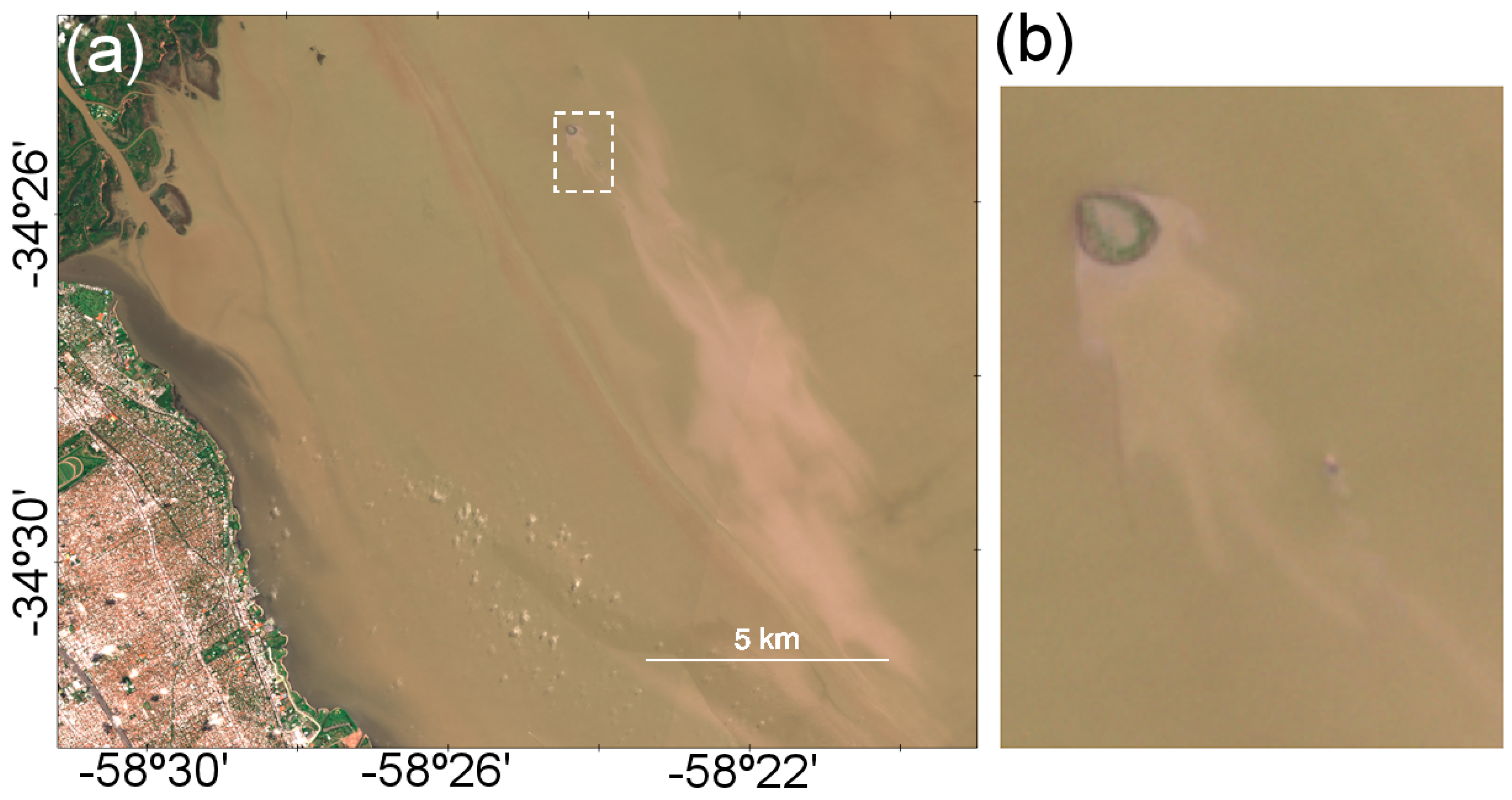
4.2. Floating Vegetation Identification
4.3. Classification Method Applied in the RdP Estuary
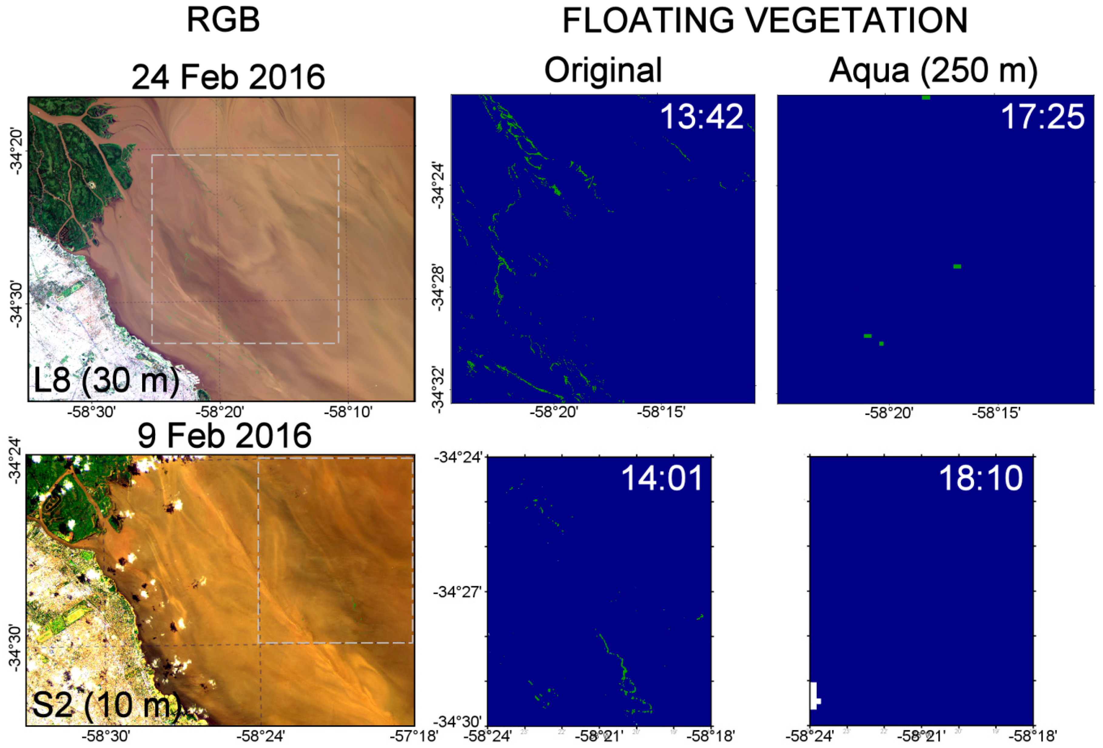
4.4. Impact of Spatial Resolution on the FV Detection
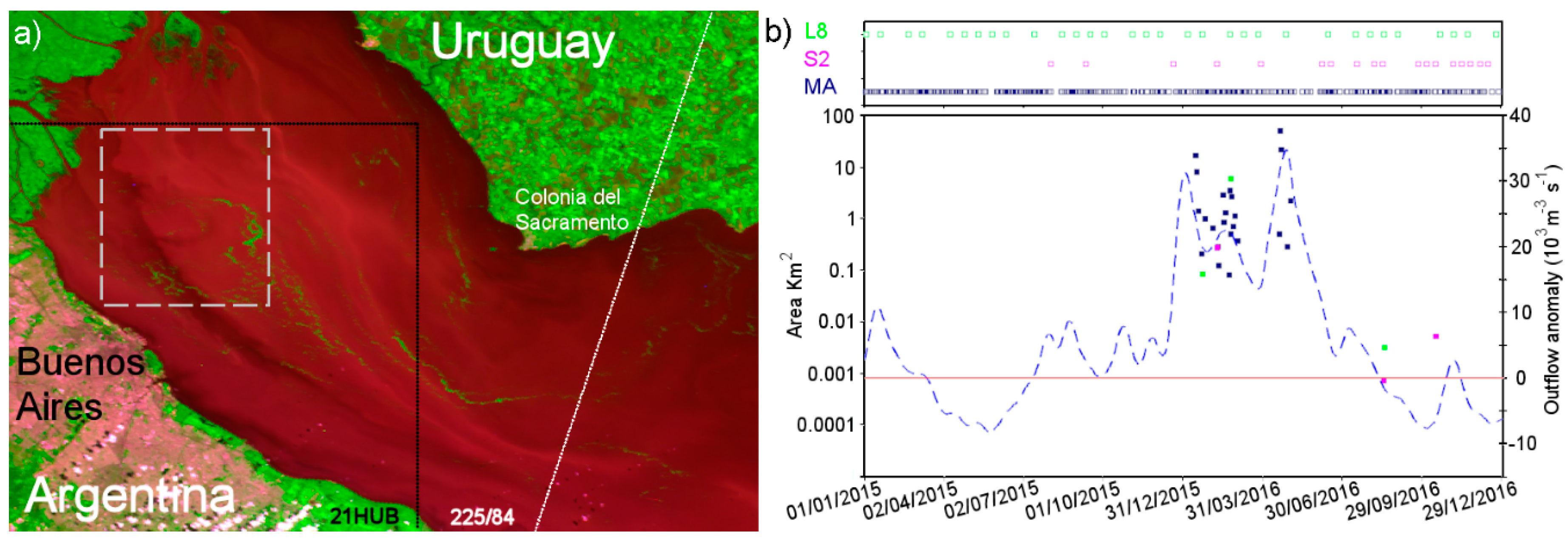
4.5. Temporal Analysis of FV Coverage
5. Conclusions
Author Contributions
Funding
Acknowledgments
Conflicts of Interest
References
- Marchetti, Z.Y.; Latrubesse, E.M.; Pereira, M.S.; Ramonell, C.G. Vegetation and its relationship with geomorphologic units in the Parana River floodplain, Argentina. J. S. Am. Earth Sci. 2013, 46, 122–136. [Google Scholar] [CrossRef]
- Fusilli, L.; Collins, M.O.; Laneve, G.; Palombo, A.; Pignatti, S.; Santini, F. Assessment of the abnormal growth of floating macrophytes in Winam Gulf (Kenya) by using MODIS imagery time series. Int. J. Appl. Earth Obs. Geoinform. 2013, 20, 33–41. [Google Scholar] [CrossRef]
- Everitt, J.H.; Alaniz, M.A.; Davis, M.R. Using spatial information technologies to detect and map waterhyacinth and hydrilla infestations in the Lower Rio Grande. J. Aquat. Plant Manag. 2003, 41, 93–98. [Google Scholar]
- Cohen, A.N.; Carlton, J.T. Accelerating invasion rate in a highly invaded estuary. Science 1998, 279, 555–558. [Google Scholar] [CrossRef] [PubMed]
- Gower, J.; Hu, C.; Borstad, G.; King, S. Ocean color satellites show extensive lines of floating Sargassum in the Gulf of Mexico. IEEE Trans. Geosci. Remote Sens. 2006, 44, 3619–3625. [Google Scholar] [CrossRef]
- Hu, C. A novel ocean color index to detect floating algae in the global oceans. Remote Sens. Environ. 2009, 113, 2118–2129. [Google Scholar] [CrossRef]
- Shi, W.; Wang, M. Green macroalgae blooms in the YellowSea during the spring and summer of 2008. J. Geophys. Res. Oceans 2009, 114, C12010. [Google Scholar] [CrossRef]
- Keesing, J.K.; Liu, D.; Fearns, P.; Garcia, R. Inter-and intra-annual patterns of Ulva prolifera green tides in the Yellow Sea during 2007–2009, their origin and relationship to the expansion of coastal seaweed aquaculture in China. Mar. Pollut. Bull. 2011, 62, 1169–1182. [Google Scholar] [CrossRef] [PubMed]
- Alawadi, F. Detection of Surface Algal Blooms Using the Newly Developed Algorithm Surface Algal Bloom Index (SABI). In Proceedings of the SPIE Remote Sensing of the Ocean, Sea Ice, and Large Water Regions 2010, Toulouse, France, 20–23 September 2010; Volume 7825, p. 782506. [Google Scholar]
- Xing, Q.; Hu, C. Mapping macroalgal blooms in the Yellow Sea and East China Sea using HJ-1 and Landsat data: Application of a virtual baseline reflectance height technique. Remote Sens. Environ. 2016, 178, 113–126. [Google Scholar] [CrossRef] [Green Version]
- Hu, L.; Hu, C.; HE, M. Remote estimation of biomass of Ulva prolifera macroalgae in the Yellow Sea. Remote Sens. Environ. 2017, 192, 217–227. [Google Scholar] [CrossRef]
- Hu, C.; Feng, L.; Hardy, R.F.; Hochberg, E.J. Spectral and spatial requirements of remote measurements of pelagic Sargassum macroalgae. Remote Sens. Environ. 2015, 167, 229–246. [Google Scholar] [CrossRef]
- Liang, Q.; Zhang, Y.; Ma, R.; Loiselle, S.A.; Li, J.; Hu, M. A MODIS-Based Novel Method to Distinguish Surface Cyanobacterial Scums and Aquatic Macrophytes in Lake Taihu. Remote Sens. 2017, 9, 133. [Google Scholar] [CrossRef]
- Minotti, P.; Ramonell, C.; Kandus, P. Regionalización del Corredor Fluvial Paraná-Paraguay. In Inventario de los Humedales de Argentina: Sistemas de Paisajes de Humedales del Corredor FluvialParaná-Paraguay, 1st ed.; Benzaquén, L., Blanco, D.E., Bó, R.F., Kandus, P., Lingua, G.F., Minotti, P., Quintana, R.D., Sverlij, S., Vidal, L., Eds.; Secretaría de Ambiente y Desarrollo Sustentable, Jefatura de Gabinete de Ministros de la Nación: Buenos Aires, Argentina, 2013; pp. 33–90. ISBN 978-987-29340-0-2. [Google Scholar]
- World Water Assessment Programme. La Plata Basin Case Study. Final Report. UNESCO. Available online: unesdoc.unesco.org/images/0015/001512/151252e.pdf (accessed on 27 April 2018).
- Robertson, A.W.; Mechoso, C.R. Interannual and decadal cycles in river flows of southeastern South America. J. Clim. 1998, 11, 2570–2581. [Google Scholar] [CrossRef]
- Jaime, P.R.; Menéndez, A.N. Análisis del Régimen Hidrológico de Los Ríos Paraná y Uruguay. Informe LHA-01-216-02; INA, 1997. Available online: https://www.ina.gov.ar/legacy/pdf/LH-Info_FRE_LHA-01-216-02_FrePlata-ParanaUruguay_Jun_2002.pdf (accessed on 27 April 2018).
- Neiff, J.J.; Malvárez, I. Grandes Humedales Fluviales. In Bases Ecológicas Para la Clasificación e Inventario de Humedales en Argentina, 1st ed.; Malvárez, I., Bó, R.F., Eds.; FCEN; Universidad de Buenos Aires; RAMSAR; USFWS; USDS: Buenos Aires, Argentina, 2004; pp. 77–93. [Google Scholar]
- Bó, R.F. Situación Ambiental en la Ecorregión Delta e Islas del Paraná. In Situación Ambiental en la Argentina 2005, 1st ed.; Brown, A., Martínez Ortiz, U., Acerbi, M., Corcuera, J., Eds.; Fundación Vida Silvestre Argentina: Buenos Aires, Argentina, 2016; pp. 131–143. ISBN 950-9427-14-4. [Google Scholar]
- Neiff, J.J.; Iriondo, M.; Carignan, R. Large Tropical South American Wetlands: A Review; UNESCO Ecotones Workshop: Seattle, DC, USA, 1994; 15p. [Google Scholar]
- Vanhellemont, Q.; Ruddick, K. Turbid wakes associated with offshore wind turbines observed with Landsat 8. Remote Sens. Environ. 2014, 145, 105–115. [Google Scholar] [CrossRef]
- Vanhellemont, Q.; Ruddick, K. Advantages of high quality SWIR bands for ocean colour processing: Examples from Landsat-8. Remote Sens. Environ. 2015, 161, 89–106. [Google Scholar] [CrossRef]
- Dogliotti, A.I.; Ruddick, K.G.; Nechad, B.; Doxaran, D.; Knaeps, E. A single algorithm to retrieve turbidity from remotely-sensed data in all coastal and estuarine waters. Remote Sens. Environ. 2015, 156, 157–168. [Google Scholar] [CrossRef]
- Knaeps, E.; Ruddick, K.G.; Doxaran, D.; Dogliotti, A.I.; Nechad, B.; Raymaekers, D.; Sterckx, S. A SWIR based algorithm to retrieve Total Suspended Matter in extremely turbid waters. Remote Sens. Environ. 2015, 168, 66–79. [Google Scholar] [CrossRef]
- Kou, L.; Labrie, D.; Chylek, P. Refractive indices of water and ice in the 0.65-2.5 μm spectral range. Appl. Opt. 1993, 32, 3531–3540. [Google Scholar] [CrossRef] [PubMed]
- Hu, C.; Lee, Z.; Ma, R.; Yu, K.; Li, D.; Shang, S. Moderate resolution imaging spectroradiometer (MODIS) observations of cyanobacteria blooms in Taihu Lake, China. J. Geophys. Res. Oceans 2010, 115, C04002. [Google Scholar] [CrossRef]
- CIE/ISO (Commission Internationale de l’Eclairage). Colorimetry—Part 5: CIE 1976 L*u*v* Colour Space and u’, v’ Uniform Chromaticity Scale Diagram, 1st ed.; International Standard ISO/CIE: Geneva, Switzerland, 2016. [Google Scholar]
- Dogliotti, A.I.; Gossn, J.I.; Vanhellemont, Q.; Ruddick, K. Large Invasion of Floating Aquatic Plants in the Río de la Plata Estuary! In Proceedings of the Ocean Optics XXIII Conference, Victoria, BC, Canada, 23–28 October 2016; Available online: http://www.iafe.uba.ar/wordpress/filesMarine/Conferences/2016_Dogliotti_etal_OO.pdf (accessed on 6 July 2018).
- Cui, T.; Zhang, J.; Sun, L.; Jia, Y.; Zhao, W.; Wang, Z.; Meng, J. Satellitemonitoring of massive green macroalgae bloom (GMB): Imagingability comparison of multi-source data and drifting velocityestimation. Int. J. Remote Sens. 2012, 33, 5513–5527. [Google Scholar] [CrossRef]
- Xu, Q.; Zhang, H.; Cheng, Y. Multi-sensor monitoring of Ulva prolifera blooms in the YellowSea using different methods. Front. Earth Sci. 2016, 10, 378–388. [Google Scholar] [CrossRef]
- Dogliotti, A.I.; Ruddick, K.; Guerrero, R. Seasonal and inter-annual turbidity variability in the Río de la Plata from 15 years of MODIS: El Niño dilution effect. Estuar. Coast. Shelf Sci. 2016, 182, 27–39. [Google Scholar] [CrossRef]
- Oyama, Y.; Matsushita, B.; Fukushima, T. Distinguishing surface cyanobacterial blooms and aquatic macrophytes using Landsat/TM and ETM+ shortwave infrared bands. Remote Sens. Environ. 2015, 157, 35–47. [Google Scholar] [CrossRef]
- Qi, L.; Hu, C.; Duan, H.; Cannizzaro, J.; Ma, R. A novel MERIS algorithm to derive cyanobacterial phycocyanin pigment concentrations in a eutrophic lake: Theoretical basis and practical considerations. Remote Sens. Environ. 2014, 154, 298–317. [Google Scholar] [CrossRef]


| Spatial Resolution (m) | RED (BW) | GREEN (BW) | BLUE (BW) | NIR (BW) | SWIR (BW) | Swath (km) | Revisit | |
|---|---|---|---|---|---|---|---|---|
| MODIS/Aqua | 250 1 & 500 2 | 645 1 (50) | 555 2 (20) | 469 2 (20) | 859 1 (250) | 1240 2 (20) | 2330 | Daily |
| L8/OLI | 30 | 655 (50) | 561 (75) | 483 (65) | 865 (40) | 1650 (100) | 180 | 8 or 16 days |
| S2A/MSI | 10 3 & 20 4 | 665 3 (30) | 560 3 (35) | 497 3 (65) | 865 4 (20) | 1610 4 (90) | 290 | 10 days |
| 100%W | FAI 0%W | Min% | 100%W | RED 0%W | Min% | 100%W | La*b* 0%W | Min% | FAIT Min% | |
|---|---|---|---|---|---|---|---|---|---|---|
| TW | −0.0336 | 0.2686 | 11.1 | 0.0834 | 0.043 | 9.1 | 10.6957 | −26.418 | 28.3 | 28.3 |
| MT | −0.0413 | 0.2686 | 13.4 | 0.1345 | 0.043 | 61.2 | 15.2198 | −26.418 | 51.8 | 61.2 |
| DRG | 0.0175 | 0.2686 | N/A | 0.1053 | 0.043 | 42.3 | 17.1252 | −26.418 | 40.0 | 42.3 |
| XTW | 0.0596 | 0.2686 | N/A | 0.1235 | 0.043 | 55.8 | 30.3149 | −26.418 | 56.2 | 56.2 |
| N | Total FV Area (Km2) | N2015 | N2016 |
|---|---|---|---|
| MA | 114.0 | 185 | 158 |
| L8 | 5.8 | 17 | 15 |
| S2A | 0.3 | 3 * | 15 |
© 2018 by the authors. Licensee MDPI, Basel, Switzerland. This article is an open access article distributed under the terms and conditions of the Creative Commons Attribution (CC BY) license (http://creativecommons.org/licenses/by/4.0/).
Share and Cite
Dogliotti, A.I.; Gossn, J.I.; Vanhellemont, Q.; Ruddick, K.G. Detecting and Quantifying a Massive Invasion of Floating Aquatic Plants in the Río de la Plata Turbid Waters Using High Spatial Resolution Ocean Color Imagery. Remote Sens. 2018, 10, 1140. https://doi.org/10.3390/rs10071140
Dogliotti AI, Gossn JI, Vanhellemont Q, Ruddick KG. Detecting and Quantifying a Massive Invasion of Floating Aquatic Plants in the Río de la Plata Turbid Waters Using High Spatial Resolution Ocean Color Imagery. Remote Sensing. 2018; 10(7):1140. https://doi.org/10.3390/rs10071140
Chicago/Turabian StyleDogliotti, Ana I., Juan I. Gossn, Quinten Vanhellemont, and Kevin G. Ruddick. 2018. "Detecting and Quantifying a Massive Invasion of Floating Aquatic Plants in the Río de la Plata Turbid Waters Using High Spatial Resolution Ocean Color Imagery" Remote Sensing 10, no. 7: 1140. https://doi.org/10.3390/rs10071140