Article

Intercomparison of Three Two-Source Energy Balance Models for Partitioning Evaporation and Transpiration in Semiarid Climates

1
State Key Laboratory of Simulation and Regulation of Water Cycle in River Basin, Beijing 100038, China
2
Research Center on Flood and Drought Disaster Reduction of the Ministry of Water Resources, China Institute of Water Resources and Hydropower Research, Beijing 100038, China
3
Guangdong Provincial Key Laboratory of Urbanization and Geo-simulation, School of Geography and Planning, Sun Yat-sen University, Guangzhou 510275, China
4
Key Laboratory of Water Cycle & Related Land Surface Processes, Institute of Geographic Sciences and Natural Resources Research, Beijing 100101, China
*
Author to whom correspondence should be addressed.
Remote Sens. 2018, 10(7), 1149; https://doi.org/10.3390/rs10071149
Submission received: 10 May 2018 / Revised: 9 July 2018 / Accepted: 18 July 2018 / Published: 20 July 2018
(This article belongs to the Special Issue Remote Sensing of Evapotranspiration (ET))

Abstract

:
Evaporation (E) and transpiration (T) information is crucial for precise water resources planning and management in arid and semiarid areas. Two-source energy balance (TSEB) methods based on remotely-sensed land surface temperature provide an important modeling approach for estimating evapotranspiration (ET) and its components of E and T. Approaches for accurate decomposition of the component temperature and E/T partitioning from ET based on TSEB requires careful investigation. In this study, three TSEB models are used: (i) the TSEB model with the Priestley-Taylor equation, i.e., TSEB-PT; (ii) the TSEB model using the Penman-Monteith equation, i.e., TSEB-PM, and (iii) the TSEB using component temperatures derived from vegetation fractional cover and land surface temperature (VFC/LST) space, i.e., TSEB-TC-TS. These models are employed to investigate the impact of component temperature decomposition on E/T partitioning accuracy. Validation was conducted in the large-scale campaign of Heihe Watershed Allied Telemetry Experimental Research-Multi-Scale Observation Experiment on Evapotranspiration (HiWATER-MUSOEXE) in the northwest of China, and results showed that root mean square errors (RMSEs) of latent and sensible heat fluxes were respectively lower than 76 W/m2 and 50 W/m2 for all three approaches. Based on the measurements from the stable oxygen and hydrogen isotopes system at the Daman superstation, it was found that all three models slightly overestimated the ratio of E/ET. In addition, discrepancies in E/T partitioning among the three models were observed in the kernel experimental area of MUSOEXE. Further intercomparison indicated that different temperature decomposition methods were responsible for the observed discrepancies in E/T partitioning. The iterative procedure adopted by TSEB-PT and TSEB-PM produced higher LEC and lower TC when compared to TSEB-TC-TS. Overall, this work provides valuable insights into understanding the performances of TSEB models with different temperature decomposition mechanisms over semiarid regions.

Graphical Abstract

1. Introduction

Evapotranspiration (ET) observations and modeling are crucial in water cycle studies [1,2,3,4]. Water scarcity is one of the main factors constraining agricultural development in arid or semiarid areas. The knowledge of ET, as well as the mechanism of ET partitioning into evaporation (E) and transpiration (T), is very important for precise quantification of the water balance in water resources planning and management, optimizing crop production, identifying crop stress and drought impacts, and evaluating the effects of climate change on water yields [5,6,7,8,9]. As satellite remote sensing is widely used to obtain information on the regional water and heat balance, it has been used to derive several global multi-decadal ET datasets that arouse extensive concern [10,11,12,13,14,15].
Over the last few decades, several remote sensing-based ET models have been proposed to estimate regional surface heat fluxes via satellite-derived land surface temperature (LST) [5,6,16,17,18,19,20]. Specifically, a one-source model, such as the Surface Energy Balance Algorithm for Land (SEBAL) [16,17], Simplified Surface Energy Balances Index (S-SEBI) [21], Surface Energy Balance System (SEBS) [20,22], and Mapping EvapoTranspiration at high Resolution with Internalized Calibration (METRIC) [5,6], often use LST and empirical resistance corrections to estimate surface heat fluxes. Two-source models, such as the two-source energy balance model (TSEB) [19], the two-source time-integrated model (TSTIM) [23], Pixel Component Arranging and Comparing Algorithm (PCACA) [24], and the enhanced two-source evapotranspiration model for land (ETEML) [25] were developed to make use of LST to estimate a sensible heat flux (H) and latent heat flux (LE) for the soil and canopy separately. Other alternative practical approaches have been proposed based on vegetation fractional cover and LST (VFC/LST) space [26,27]. Related research includes the work by Moran et al. [28], Jiang and Islam [29,30], Stisen et al. [31], and Shu et al. [32]. Extensive reviews of remote sensing-based methodologies on surface heat flux estimation can be found in the works of Courault et al. [33], Kalma et al. [34] and Li et al. [35].
As an appealing modeling scheme, two-source energy balance models can estimate evapotranspiration (ET), evaporation (E), and transpiration (T) of vegetated surfaces, which has important applications in water resources management for irrigated crops in arid and semiarid areas [36]. To estimate E and T separately, the soil temperature (TS) and canopy temperature (TC) need to be accurately measured or derived, making temperature decomposition the core of the two-source modeling approach. Generally, four categories of methods have been developed to decompose remotely-sensed temperature into soil and canopy temperatures. (1) The first category calculates soil and vegetation component temperatures using dual- or multi-angular thermal infrared measurements [37]. For instance, a dual-source model using bi-angular thermal infrared measurements was developed by Jia [38] and Jia et al. [39]. However, currently limited sensors have bi- or multi-angular thermal infrared channels and thus constrained the availability of remote sensing data source in this category of method. (2) The second category assumed that LST is the sum of vegetation and soil temperatures weighted by the vegetation fractional cover (fc), i.e., LST f c T C + T S ( 1 f c ) . This kind of method assumed that the LST of a highly vegetated pixel in the neighborhood would be a reasonable approximation of TC, and a selected neighborhood area of the target pixel based on certain thresholds in the corresponding NDVI image [40,41]. As TC is approximately determined, TS can be derived accordingly using T S = ( LST f c T C ) / ( 1 f c ) . (3) The third category retrieves component temperatures using an iterative procedure based on an energy balance and resistance network. Typically, the TSEB model proposed by Norman et al. [19] uses a system of temperature gradient-resistance equations that are solved by an iterative procedure, in which an initial estimate of plant transpiration is determined by the Priestley-Taylor equation (TSEB-PT). The procedure terminates when soil evaporation (LEs) exceeds zero, and Tc and Ts are recalculated until energy balance closure is reached. Recently, TSEB was revised by Colaizzi et al. [42] and Colaizzi et al. [43] using the Penman-Monteith equation (TSEB-PM) instead of the Priestley-Taylor equation in order to characterize vegetation transpiration, and this revised version was found to be more applicable for advective semiarid climates. (4) The fourth category derives component temperatures based on VFC/LST space [24,28,44,45]. Moran et al. [28] introduced a water deficit index (WDI) based on the VFC/LST trapezoid space and extended the application of a crop water stress index (CWSI) over fully- to partially-vegetated surface areas. Zhang et al. [24] proposed a method to retrieve land surface component temperatures based on the interpretation of soil wetness isolines within a VFC/LST trapezoidal space. The main assumption of this method is that the isolines in the VFC/LST trapezoid space is mainly controlled by soil water availability and the isolines within a VI/LST trapezoidal space are used to decompose the composite temperature into component temperatures. This method was recently revised and adopted by Sun et al. [46], Long and Singh [47], Yang and Shang [48], Yang et al. [25], and Sun [49] to develop two-source models.
Combined with satellite remote sensing, the TSEB models have been extensively used to estimate regional ET. However, how the accuracy of ET estimations from TSEB models is affected by its component temperature estimation and E/T partitioning are rarely reported, and requires careful study. The objective of this study is to evaluate the capabilities of three TSEB models in predicting surface fluxes under various ranges of soil moisture contents, and then analyze how the different performances of three models are attributed to the different adopted schemes in component temperature decomposition and E/T partitioning. Section 2 presents the description of the three two-source models: TSEB-PT, TSEB-PM, and TSEB-TC-TS. Section 3 introduces the pertinent experiment campaign in the study area, i.e., Heihe Watershed Allied Telemetry Experimental Research-The Multi-Scale Observation Experiment on Evapotranspiration (HiWATER-MUSOEXE) Campaign, remotely-sensed data used for driving the TSEB models, and the ground measurements for the models’ assessment. Section 4 first reports the fluxes estimation accuracies from three TSEB models with retrievals from ASTER imagery. In Section 4.2, E/T partitioning is intercompared within three models and evaluated against the benchmark obtained using the stable oxygen and hydrogen isotopes technique. In the remainder of Section 4, intercomparison using component temperatures generated from three models was conducted to further investigate the uncertainty in E/T partitioning. Section 5 discusses the advantages and limitations in this work, and the final section provides a conclusion.

2. Theory and Methodology

2.1. TSEB-PT Model

The TSEB model was originally developed by Norman et al. [19] to make use of remotely-sensed radiometric surface temperatures to estimate soil evaporation and canopy transpiration. This model has been modified by Kustas and Norman [50,51] through improving the soil surface resistance formulation and net radiation partitioning between the soil and canopy components. The net radiation is partitioned between the vegetated canopy and soil, and can be expressed as:
R n = R ns + R nc = H + L E + G
where R n is net radiation (W/m2), R ns and R nc are the net radiation for soil and vegetation canopy (W/m2), respectively; H and LE are the sensible and latent heat fluxes (W/m2), respectively, and G is the soil heat flux (W/m2). The energy balance for the soil and vegetated canopy can be expressed as:
R ns = H s + L E s + G
R nc = H c + L E c
where H s and H c are the sensible heat fluxes for the soil and canopy respectively (W/m2), L E s and L E c are the latent heat fluxes for the soil and canopy, respectively (W/m2). G is parameterized with the phase-difference approach proposed by Santanello and Friedl [52]:
G = R ns { a · cos [ 2 π b ( t + c ) ] }
where t is the solar time angle (s), a is the amplitude parameter (dimensionless), b is the period length (s), and c is the shift (s). In this study, parameters a, b, and c take the values of 0.3, 86,400, and 10,800 following Colaizzi et al. [43] and Song et al. [53].
In this study, the series resistance network form was applied, in which Hc, Hs, and the sum of both terms are calculated as:
H c = ρ C P T C T AC r x
H s = ρ C P T S T AC r s
H = ρ C P T AC T A r A
where ρ is the air density (kg/cm3), C P is the specific heat of air (J/kg/K), T S is the soil temperature (K), T C is the canopy temperature (K), T AC and T A are the air temperature within the canopy boundary layer and air temperature (K), respectively, r A is the aerodynamic resistance (s/m), r x is the resistance in the boundary layer near the canopy (s/m), and r s is the resistance to heat flux in the boundary layer above the soil surface (s/m). r A , r x , and r s are calculated according to Norman et al. [19] and Kustas and Norman [50].
The TSEB-PT model uses a modified Priestley-Taylor formulation to parameterize the canopy transpiration:
L E c = α PT f G Δ Δ + γ R nc
where α PT is the Priestley-Taylor parameter (dimensionless), f G is the fraction of green vegetation (dimensionless), Δ is the slope of the saturation vapor pressure versus temperature curve (kPa/°C), and γ is the psychrometric constant (kPa/°C). An initial estimate of T C can be derived as follows:
T c = T A + R nc r A ρ C P [ 1.0 α PT f G Δ Δ + γ ]
Accordingly, T S is calculated with an initial estimate of T S , and then r s can be estimated with the temperature gradient between the soil and canopy described in Kustas and Norman [51]. From Equations (5) to (8), the component sensible heat flux HS can be calculated and latent heat fluxes from canopy LEC and soil surface LES are solved as residual terms. In order to obtain a realistic estimation of surface heat fluxes under water stressed conditions, the α PT is iteratively decreased until LEs exceeds zero. The detailed description of the TSEB model and the parameterization of the resistance network can be found in Norman et al. [19] and Kustas and Norman [51].

2.2. TSEB-PM Model

The TSEB model was revised by Colaizzi et al. [42] and Colaizzi et al. [43] using the Penman-Monteith equation instead of the Priestley-Taylor formulation to account for the impact of advection over semiarid climates. This revised version of the TSEB model is termed TSEB-PM. The effects of varying the vapor pressure deficit can thus be taken into account in the TSEB-PM model. The canopy transpiration is characterized using the Penman-Monteith equation:
L E c = f G ( Δ R nc Δ + γ * + ρ C P ( e s e a ) r A ( Δ + γ * ) )
and T c is initialized as follows:
T C = T A + R nc r A γ * ρ C P ( Δ + γ * ) e s e a Δ + γ *
where γ * = γ ( 1 + r c / r A ) , r c is the bulk canopy resistance (s/m), r A is the aerodynamic resistance between the canopy and the air above the canopy (s/m), and e a and e s are the actual and saturation vapor pressure of the air (kPa), respectively. Similar to TSEB-PT, the TSEB-PM model was iteratively implemented as described in Section 2.1. During the iterative procedure, r c increases from 10 s/m with an increment of 20 s/m and terminates at 5000 s/m, or until LEs exceeds zero. The comprehensive introduction of the TSEB-PM can be found in Colaizzi et al. [42] and Colaizzi et al. [43].

2.3. TSEB-TC-TS Model

TSEB was modified by Kustas and Norman [54] to calculate turbulent heat fluxes using canopy and soil component temperatures that were measured or derived from other methods. This modified TSEB model is called TSEB-TC-TS in this study. The Priestley-Taylor iteration procedure is not applied in TSEB-TC-TS, but the remainder of the physical framework of TSEB-TC-TS is identical to that of TSEB-PT. The within-canopy temperature (TAC) is estimated from derived component temperatures as follows:
T AC = T A r A + T s r s + T C r x 1 r A + 1 r s + 1 r x
Consequently, the component sensible heat fluxes HS and HC are directly calculated from Equations (5) and (6), and the component latent heat fluxes LEC and LES are calculated as residual terms from Equations (2) and (3).
The VFC/LST space is adopted to retrieve component temperatures by Zhang et al. [24], Zhang et al. [55], Sun et al. [40], Merlin et al. [44], and Merlin et al. [45]. Based on the theoretical determination of the dry and wet edges of the VFC/LST space, this method was further revised and adopted by Long and Singh [47] and Yang and Shang [48] to develop two-source models. In the traditional method, the VFC/LST trapezoid is mainly determined manually based on the 2-D VFC/LST scatter plot, which would cause great uncertainty. Recently, Yang et al. [25] improved this method and proposed to make use of the VFC/LST trapezoid space for each pixel. Different from traditional method, the four theoretical points for each pixel are determined based on an energy balance model and the Penman-Monteith equations. In this study, this pixel-wise surface temperature decomposition method is adopted. The employed VFC/LST space is determined with four theoretical points using the following equations from Moran et al. [28].
For the vertex of dry bare soil, the difference between LST and Ta can be derived as follows:
( T S T a ) max = [ r a ( R n G ) / ρ a C p ]
For the vertex of saturated bare soil,
( T S T a ) min = [ ( r a ( R n G ) ) / ( ρ a C p ) ] [ γ / ( Δ + γ ) ] [ V P D / ( Δ + γ ) ]
For the vertex of well-watered fully-cover vegetation,
( T C T a ) min = [ ( r a ( R n G ) ) / ( ρ a C p ) ] [ γ ( 1 + r cp / r a ) / ( Δ + γ ( 1 + r cp / r a ) ) ] [ V P D / ( Δ + γ ( 1 + r cp / r a ) ) ]
For the vertex of water-stressed fully-cover vegetation,
( T C T a ) max = [ ( r a ( R n G ) ) / ( ρ a C p ) ] [ γ ( 1 + r cx / r a ) / ( Δ + γ ( 1 + r cx / r a ) ) ] [ V P D / ( Δ + γ ( 1 + r cx / r a ) ) ]
where VPD (kPa) is the vapor pressure deficit of the air at temperature T a , γ is the psychrometric constant (kPa/°C), and r a is aerodynamic resistance (s/m) estimated with the equations proposed by Thom [56]. r cp is the canopy resistance at potential evapotranspiration (s/m), and r cx is the maximum canopy resistance (s/m). As such, a VFC/LST trapezoid space is determined for each pixel and the measurements of (LST-Ta) and the fractional vegetation cover would be located within the trapezoid space.
Based on the VFC/LST trapezoid space determined above, the composite radiometric surface temperature of each pixel can be decomposed to soil and canopy component temperatures [24,25,55]:
T S T a = ( LST T a ) K s f c
T C T a = K s ( 1 f c ) + ( LST T a )
where K s is the slope of the isoline that passes through the point located in VFC/LST space, and can be derived by interpolating the slope of the warm edge and that of the cold edge. The detailed description of this method can be found in Yang et al. [25]. Once TS and TC are determined, the component fluxes in TSEB-TC-TS can be estimated.
In addition to TS and TC, TSEB models can estimate evaporation (E) and transpiration (T) of vegetated surface, such information can be used to calculate component water stress of vegetation and soil. Following the equations from Yang et al. [25], the crop water stress index for the canopy component (CWSIc) and soil water deficit index for soil component (SWDIS) are calculated as follows:
C W S I C = 1 L E c / E P c
S W D I s = 1 L E s / E P s
E P c and E P s are the potential transpiration rate and potential soil evaporation rate, respectively.

3. Study Area and Data Processing

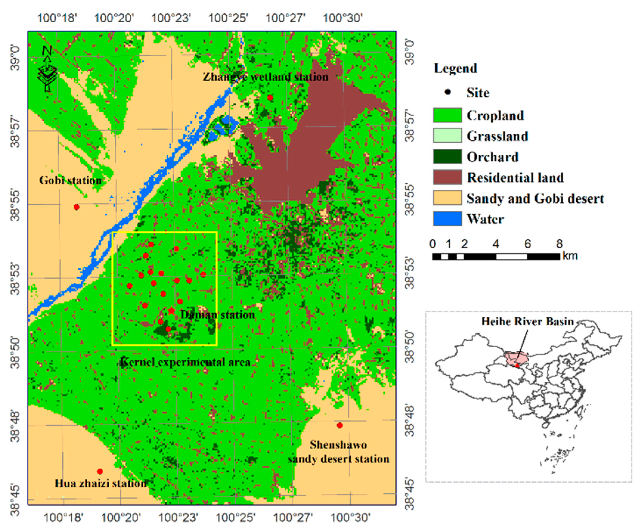
3.1. HiWATER-MUSOEXE Campaign and Ground-Based Measurements

Heihe Watershed Allied Telemetry Experimental Research (HiWATER) was performed at the Heihe River Basin of northwestern China with airborne, satellite-borne, and ground-based remote sensing experiments at various scales during 2012–2015 [57]. As one of most important thematic experiments of the HiWATER, the Multi-Scale Observation Experiment on Evapotranspiration (MUSOEXE) over the Zhangye oasis provided multiscale data sets of meteorological elements and land surface parameters that facilitate the development and validation of ET models over heterogeneous surfaces [58,59]. Figure 1 shows the distribution of flux towers and the land use classifications in the MUSOEXE.
MUSOEXE involved a multi-scale observation campaign over heterogeneous surfaces by using an observation matrix composed of 21 stations. Each station was equipped with a set of eddy covariance (EC) system and automatic weather system (AWS). Turbulent heat fluxes are measured with EC system and the raw data were processed using EdiRe software and averaged over 30 min. Wind speed, wind direction, air temperature, vapor pressure, net radiation, and atmospheric pressure were measured in AWS with 10-min intervals. The soil heat fluxes were measured using three heat flux plates located 6 cm below the ground’s surface at each site. In order to better represent the surface soil heat flux, the Thermal Diffusion Equation and Correction (TDEC) method proposed by Yang and Wang [60] was applied to correct the observed soil heat flux with the observed soil moisture and temperature profile. The residual method [61] was adopted to adjust sensible and latent heat fluxes by forcing the energy balance closure.
The isotopic composition of atmospheric water vapor provided rich information on the hydrological cycle and gaseous exchange processes between the terrestrial vegetation and atmosphere. Due to technical and instrumental limitations, the measurements of the isotopic composition of water vapor were limited to discrete campaigns and discrete samples. During the HiWATER program, the isotopic composition of water vapor from the surface air was measured in a corn cropland (100.3722°E, 38.8555°N) at Daman superstation using a flux gradient method, using a cavity ring-down spectroscopy (CRDS) water vapor isotope analyzer. Considering water vapor as a mixture of ET from an ecosystem that carried unique isotopic signals from plant transpiration and soil evaporation separately, the measured isotopic composition of water was used to partition ET into evaporation and transpiration. Details of the isotope experiment and its calibration procedure are given by Huang and Wen [62] and Wen et al. [63]. In this study, the ratio of T over ET was collected to evaluate the reliability of three TSEB models on evaporation and transpiration partitioning.

3.2. Remote Sensing Data and Derivation of Related Variables

In this study, nine scenes from the Advance Spaceborne Thermal Emission and Reflection Radiometer (ASTER) on board Terra during the experiment period were collected. These nine scenes were acquired on 15 June, 24 June, 10 July, 2 August, 11 August, 18 August, 27 August, 3 September, and 12 September of 2012 (DOYs: 167, 176, 192, 215, 224, 231, 240, 247, 256, respectively). The LST and the land surface albedo were provided by “Heihe Plan Science Data Center, National Natural Science Foundation of China” (http://www.heihedata.org). The LST data were retrieved by Li et al. [64] using a temperature/emissivity separation (TES) algorithm proposed by Gillespie et al. [65], combined with the water vapor scaling atmospheric correction method [66]. Land surface albedo was retrieved from a Charge Coupled Device (CCD) camera on HJ-1 satellite by Sun et al. [67].
Three data sets including the visible, near-infrared (NIR) bands of ASTER and albedo from HJ-1, were all re-sampled to 90 m to be consistent with the thermal infrared band in spatial resolution. In addition, the leaf area index (LAI), crop height, and fractional vegetation cover for HiWATER-MUSOEXE were derived based on the empirical relationships proposed by Yang et al. [68].

4. Results

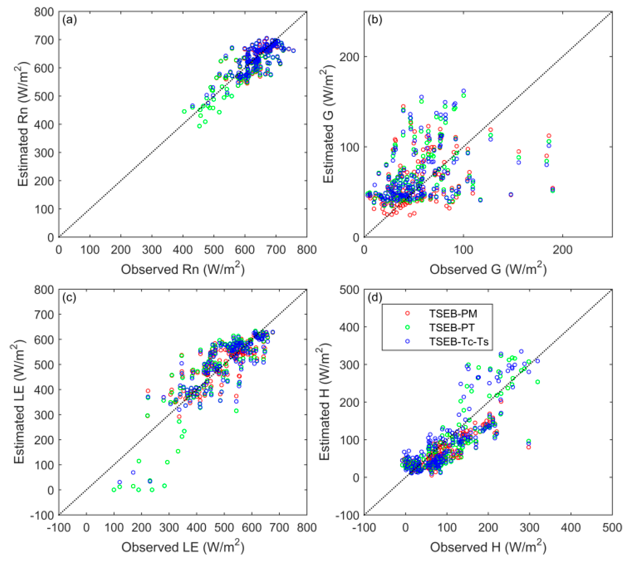
4.1. Validation of Three TSEB Models over MUSOEXE

TSEB-PT, TSEB-PM, and TSEB-TC-TS were applied to the Zhangye oasis using ground-based and satellite-derived observations introduced in Section 3, and the model performances were evaluated using flux measurements from the MUSOEXE observation matrix. As a first step of model validation, the flux estimates were averaged over the upwind source area for each flux tower [69], and flux measurements were linearly interpolated to temporally match the time of satellite overpass. Figure 2 shows the validation scatter plot for each energy balance component (Rn, G, LE, and H) from TSEB-PT, TSEB-PM, and TSEB-TC-TS estimations. Validation statistics comparing the three models’ performances are summarized in Table 1. Results show that estimated Rn from all three models were in good agreement with tower observations, and the absolute mean biases in estimated Rn for three models are all below 10 W/m2. Besides, all models slightly overestimated G, with the RMSEs all slightly exceeding 37 W/m2. Despite the different parameterization schemes used in three models (for instance, both TSEB-PT and TSEB-PM use the iterative procedure to calculate component surface temperatures, whereas TSEB-TC-TS employs the theoretical VFC/LST trapezoid for component temperature decomposition), they all exhibited comparable skills in estimation of H and LE, which can be indicated by the similar RMSEs (≈44.9–47.9 W/m2 for H, and ≈61.8–75.3 W/m2 for LE) from Table 1.
The spatial distributions of H and LE over the Zhangye oasis based on TSEB-PT, TSEB-PM, and TSEB-TC-TS for the satellite overpass on July 10 of 2012 are shown in Figure 3. Generally, the spatial patterns of surface fluxes were similar between the three models. In addition, the contrasting features over the oasis and the surrounding sandy and Gobi desert were clearly observed from all three models. Specifically, the Zhangye oasis, which mainly comprises of irrigated farmland, exhibited an average LE over 400 W/m2. On the contrary, across the sandy and Gobi desert, LE was typically below 300 W/m2 and H was over 100 W/m2.
In summary, all three employed models performed similarly in estimating H and LE despite using different schemes for modeling canopy transpiration and deriving component surface temperatures. With substantial ground observations from the tower-based network, the performances of the three models over MUSOEXE were proven reliable. The difference in derived component temperatures and partitioned evaporation and transpiration among the three models are analyzed in the following two sections.

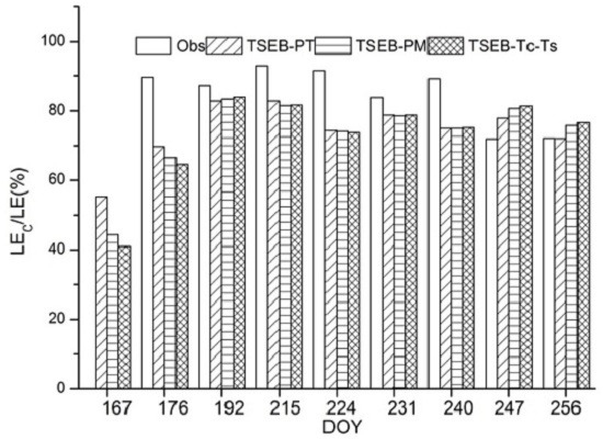
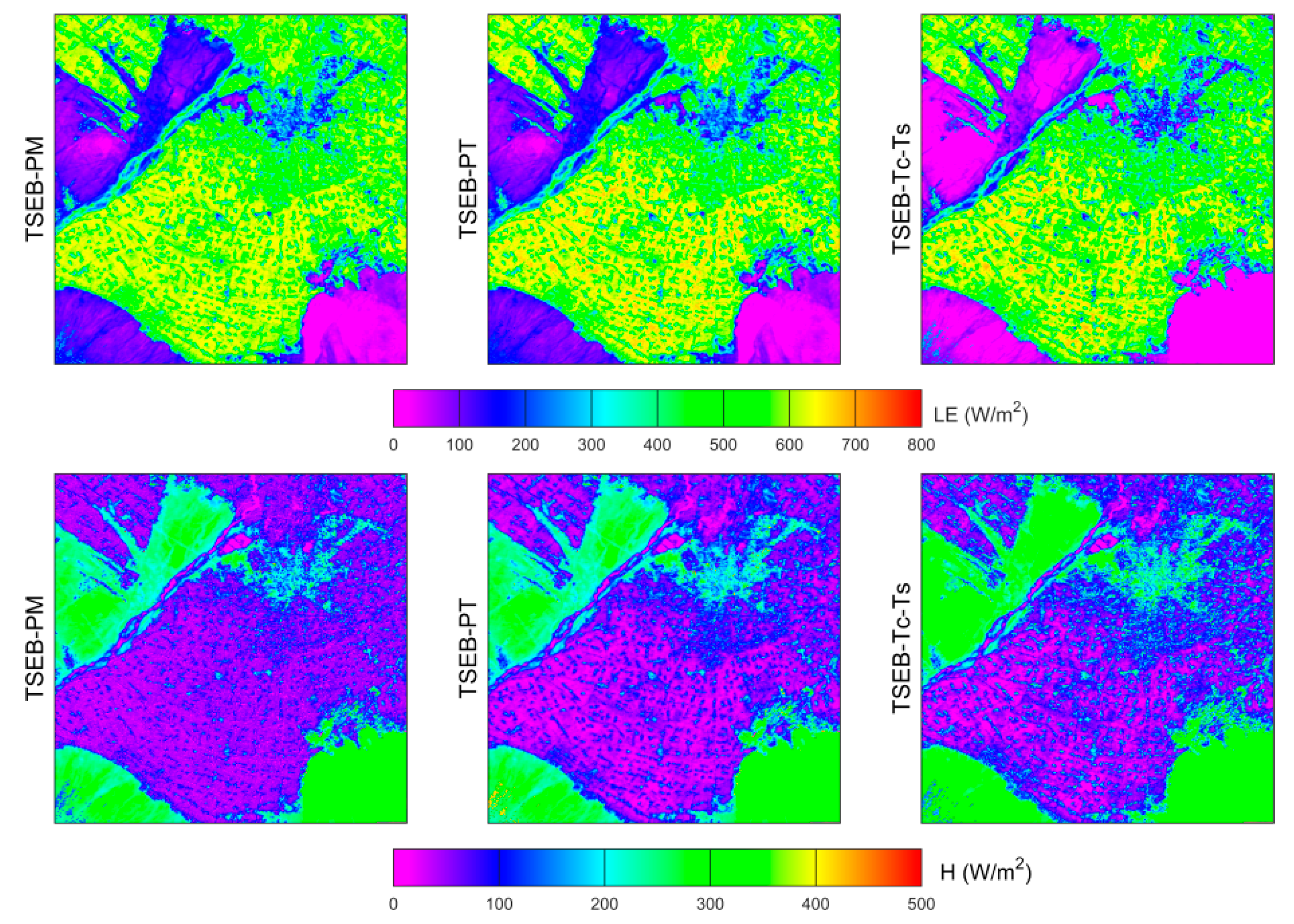
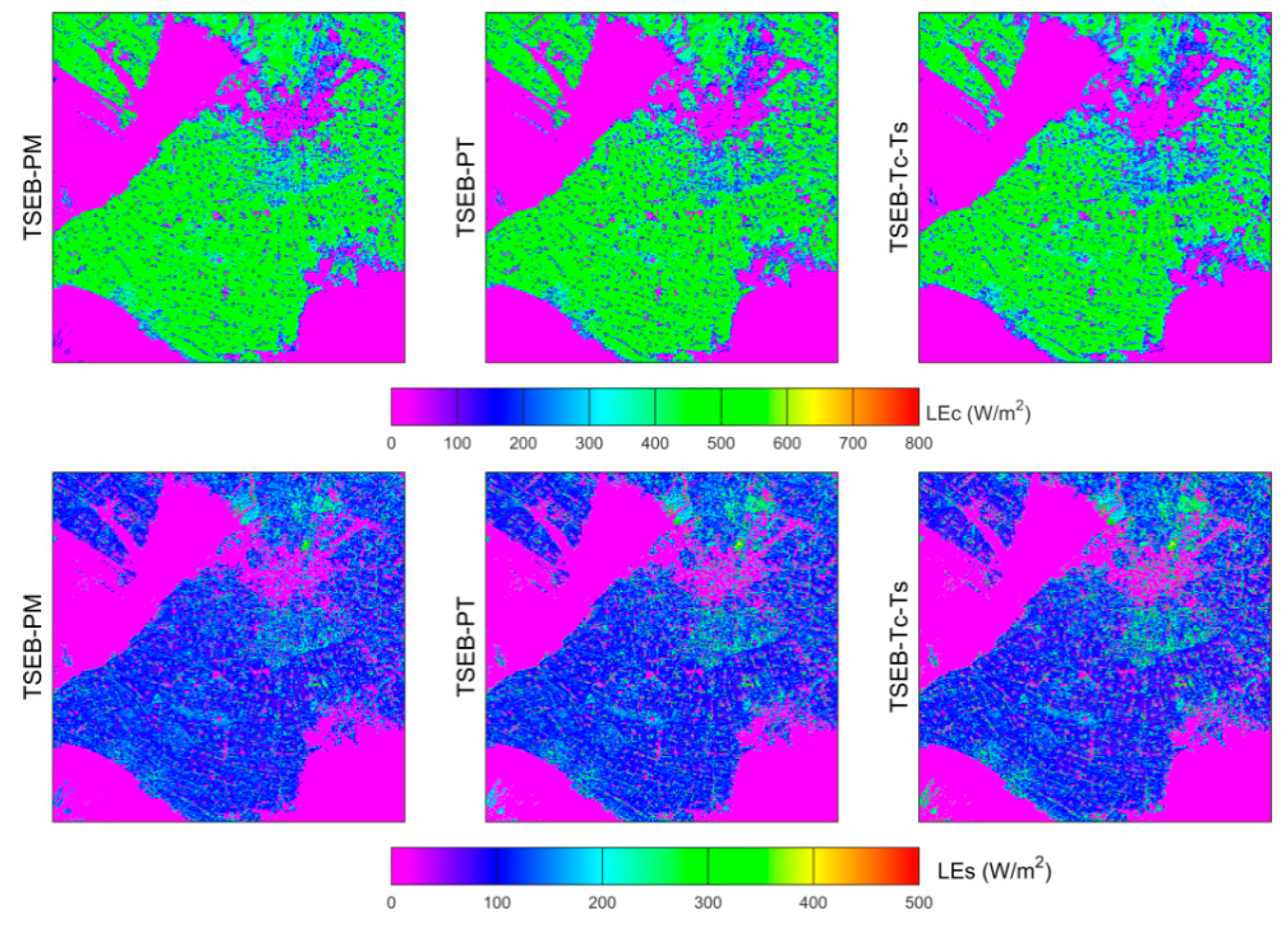
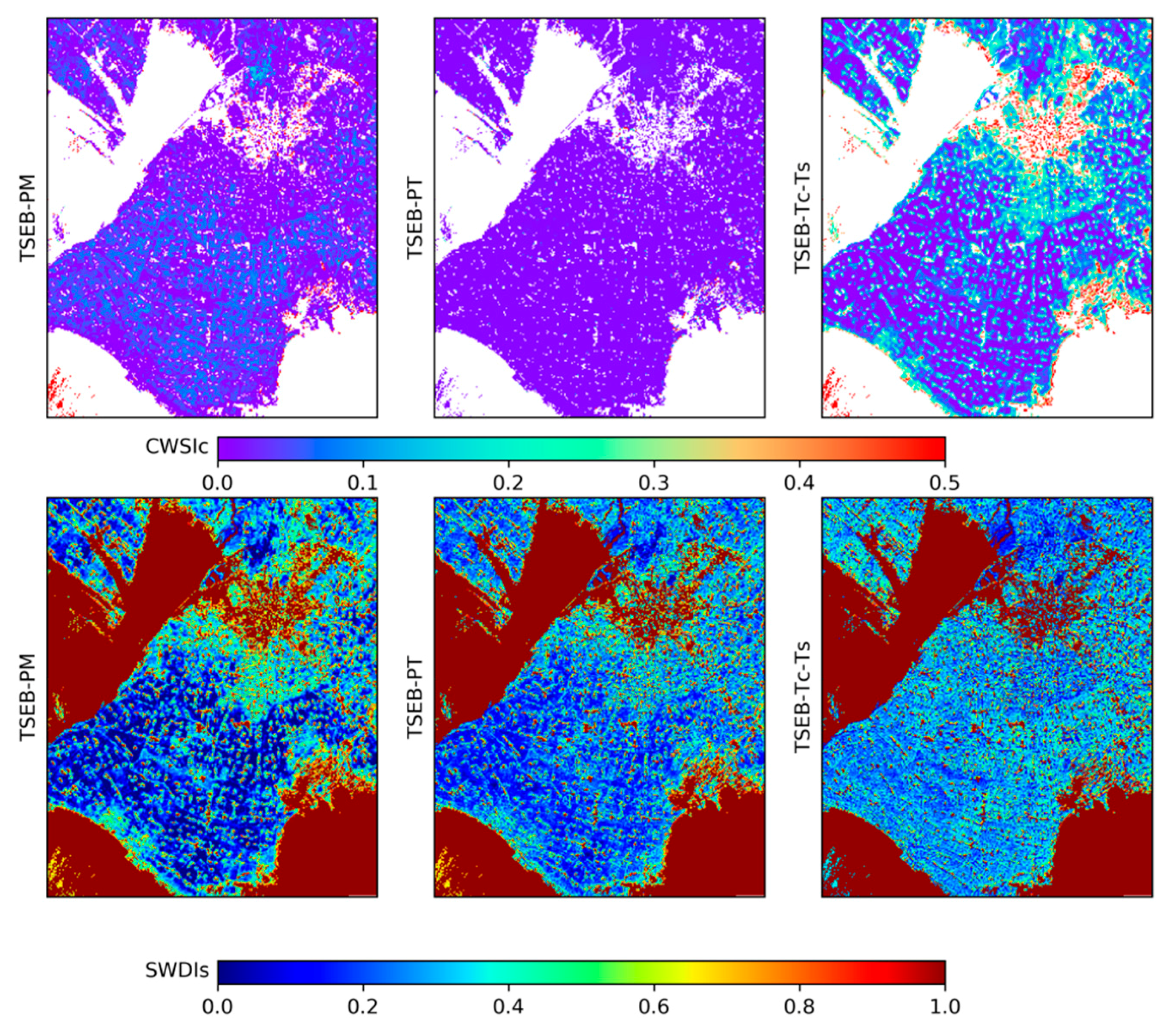
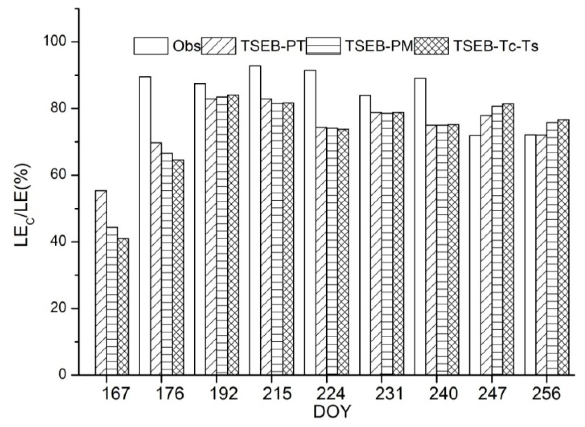
4.2. Intercomparison of E/T Partitioning from Three TSEB Models

The spatial distributions of canopy transpiration (LEc) and soil evaporation (LEs) based on TSEB-PT, TSEB-PM, and TSEB-TC-TS on 10 July of 2012 are shown in Figure 4. The spatial patterns of LEc and LEs derived from the three models are similar, and the range of LEc for irrigated farmland was about ≈350–500 W/m2. With respect to LEs, the difference derived from the three models can be visually discerned from Figure 4. In comparison with TSEB-PT and TSEB-PM, TSEB-TC-TS tended to produce higher LEs, especially over the sparsely vegetated area around the residential area and the sandy Gobi desert.
In this study, both CWSIc and SWDIs were further derived to compare the performances of the three TSEB models on detecting vegetation and soil water stresses. The spatial distributions of CWSIc and SWDIs on 10 July 2012 based on three models are shown in Figure 5. The sandy and Gobi desert pixels are masked in CWSIc images in order to more clearly reveal the difference of the three TSEB models in detecting vegetation water stress over the oasis. TSEB-PM and TSEB-PT show similar performances regarding the detection of vegetation stress with both CWSIc values close to zero. On the contrary, TSEB-TC-TS seemed to detect a higher level of vegetation water stress, with a CWSIc peak at 0.45. In addition, the spatial heterogeneity was more prominent in TSEB-TC-TS, since the CWSIc gradient in the oasis and urban areas are clearly seen from the upper right subplot of Figure 5. With respect to SWDIs, the spatial distributions were quite similar between the three TSEB models. The SWDIs values for the oasis was smaller than the surrounding sandy and Gobi desert, and the contrasting features over the oasis and the surrounding sandy and Gobi desert were clearly observed from SWDIs subplots from all three models.
The ratios of LEC/LE (i.e., T/ET) measured using the stable oxygen and hydrogen isotopes technique during HiWATER-MUSOEXE are utilized to evaluate the performances of three TSEB models on partitioning E and T. Figure 6 shows the intercomparison of LEC/LE between the three models and ground measurements. The ratios of LEC/LE were underestimated on DOYs of 176, 192, 215, 224, 231, and 240, while slight overestimation of LEC/LE occurred on DOYs of 247 and 256 in all three models. The LEC/LE ratios derived from three models were very close in most cases at this site. The mean observed LEC/LE ratio was 84.7%, while the mean estimated LEC/LE ratios were 76.7%, 76.9% and 77.0% for TSEB-PT, TSEB-PM, TSEB-TC-TS. All three models seemed to slightly underestimate the LEC/LE ratio. However, the observed LEC/LE ratios exhibited a decline during September (DOYs of 247 and 256), mainly due to leaf senescence, which was not characterized by all three models.
In order to further investigate the difference regarding E and T partitioning between the three models, a pixel-based comparison of LEC and LES in the kernel experimental area of MUSOEXE was conducted and shown in Figure 7, with color shading indicating pixel density. The statistics for a pixel-based comparison of LEC and LES in the kernel experimental area are summarized in Table 2. Most points are under the 1:1 line in Figure 7a,b, which suggests that TSEB-PM tended to produce higher LEC than TSEB-PT and TSEB-TC-TS. The mean differences (MDs) for the pairs of TSEB-PT/TSEB-PM and TSEB-TC-TS/TSEB-PM were 2.9 W/m2 and 18.1 W/m2, respectively (mean differences were calculated by subtracting the former model of the pair from the latter model). LEC estimated from TSEB-PT was comparatively higher than that from TSEB-TC-TS, with MD being 15.2 W/m2 for the TSEB-TC-TS/TSEB-PT pair. Correspondingly, comparing to TSEB-PT and TSEB-TC-TS, TSEB-PM tended to underestimate LEs as shown in Figure 7e,f, with MDs of −4.2 W/m2 and −2.8 W/m2 for the pairs of TSEB-PT/TSEB-PM and TSEB-TC-TS/TSEB-PM, respectively. The LES estimations from TSEB-PT and TSEB-TC-TS for the kernel experimental area were similar, with a correlation coefficient R being approximately 1.0, MD being 1.4 W/m2, and the mean absolute difference (MAD) being 6.2 W/m2. Since the component temperature decomposition has a major impact on E/T partitioning, to explore the mechanism underlying the observed difference on LEC (LES) from three models, a further intercomparison on the derived component temperature is conducted in the next section.

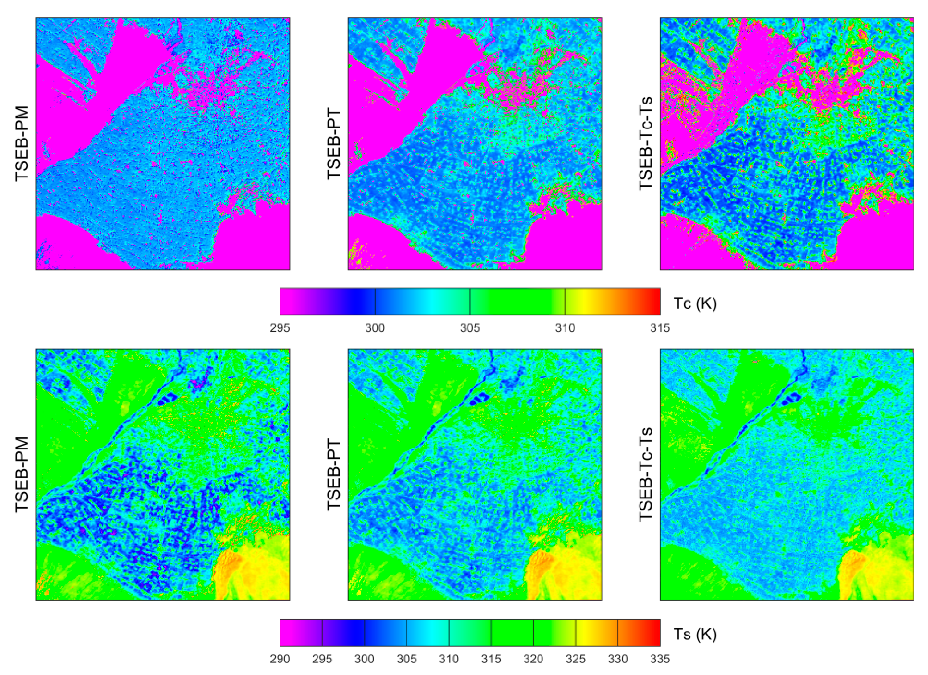
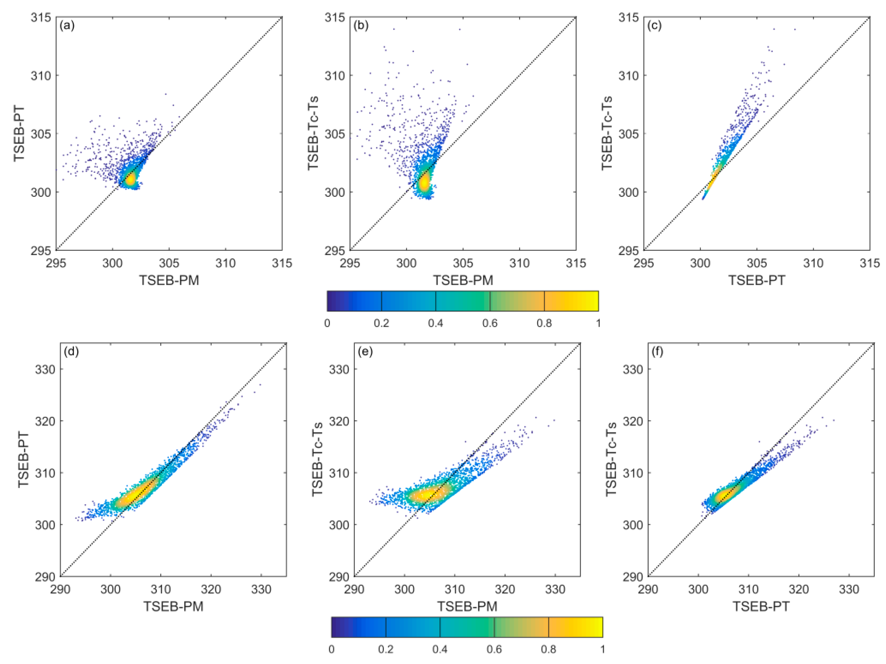
4.3. Intercomparison of Tc and Ts Derived from Three TSEB Models

Intercomparison of the component temperatures derived from the three models is shown in Figure 8. The TC derived from TSEB-PM showed a relatively homogenous pattern over the Zhangye oasis and the average of TC approximated 301 K. On the contrary, TC derived from TSEB-PT and TSEB-TC-TS showed a much larger spatial variability, and the contrast between farmland and residential area is more discernable in both models. However, the spatial contrast between farmland and residential area was less significant for the TSEB-TC-TS derived Ts (Figure 8).
A pixel-based comparison of decomposed TC and TS in the kernel experimental area was conducted and is shown in Figure 9. It is noticed that the component temperatures were much more scattered compared to the component fluxes in the scatter plot of Figure 7. The statistics for the pixel-based comparison of TC and TS in the kernel experimental area are listed in Table 3. Generally, TSEB-TC-TS estimates higher TC compared to TSEB-PT and TSEB-PM, and TSEB-PT tended to overestimate TC in relation to TSEB-PM, with the MD of TSEB-PT/TSEB-PM pair being −0.2 K.
Different strategies for deriving TC and TS were responsible for the observed differences in surface fluxes between the three modeling approaches. As previously stated, both TSEB-PT and TSEB-PM applied an iterative approach to derive component temperatures. Although the identical temperature decomposition method was applied to TSEB-PT and TSEB-PM, the component temperatures derived from both models showed a significant difference, with correlation coefficient R being only 0.13 for TC. Different from TSEB-PT and TSEB-PM, TSEB-TC-TS adopted the VFC/LST trapezoid space to estimate the component temperatures, which would explain the distinct characteristics shown in Figure 8. Specifically, for the irrigated farmland, the component temperatures derived from TSEB-TC-TS were comparable to those derived from the other two models. Due to the lack of constraint on adjusting the canopy transpiration, the vegetation component temperature from TSEB-PT and TSEB-PM would be very close to pixels in well-watered and fully-covered vegetation areas.
The scientific rationale can be explained as follows. Based on the VFC/LST space, Figure 10 illustrates the temperature decomposition methods adopted in TSEB-PT, TSEB-PM, and TSEB-TC-TS. Both TSEB-PT and TSEB-PM applied an iterative approach to derive the component temperatures and this approach assumed vegetation transpiration at the potential rate as an initial value. Due to the lack of constraint on adjusting the canopy transpiration, the vegetation component temperature from TSEB-PT and TSEB-PM would be very close to Point C (Figure 10) in well-watered and fully vegetated areas. Among TSEB-PM and TSEB-PT, the former employs the Penman-Monteith equation to consider the varying VPD under advective semiarid climates, and this would lead to higher LEC compared to TSEB-PT. Consequently, the soil component temperature from TSEB-PM was higher than that from TSEB-PT. Different from TSEB-PM and TSEB-PT, TSEB-TC-TS adopted the VFC/LST trapezoid space to estimate component temperatures. TSEB-TC-TS assumed that the vegetation and soil share the same water pool, and the slope of each isoline in the VFC/LST space could be derived by interpolating the slopes of both dry and cold edges. The temperature decomposition methods adopted in the three TSEB models is illustrated in Figure 10, the soil surface temperatures derived from TSEB-PM, TSEB-PT, and TSEB-TC-TS are denoted by Ts1, Ts2, and Ts3, and the vegetation canopy temperatures derived from the same three models are denoted by Tv1, Tv2, and Tv3. It is clear that Tv1 and Tv2 were underestimated compare to Tv3, and this led to a higher T/ET partition for TSEB-PM and TSEB-PT compared to TSEB-TC-TS, which consequently overestimated LEC when compared to TSEB-TC-TS. A component temperatures decomposition method based on isolines in the VFC/LST space provided a further constraint for vegetation transpiration and would be a good substitution for an iterative approach.

5. Discussion

5.1. Reliability of the Employed TSEB Models in Estimating Surface Fluxes

The HiWATER–MUSOEXE data have been used extensively to validate the land surface flux models, including one-source and two-source models [70,71,72]. Using the same set of ground-based observations, Ma et al. [70] applied a revised SEBS model to estimate regional heat fluxes in the Heihe River Basin, and their assessment indicates that the RMSEs of the modeled H and LE are 56.9 W/m2 and 74.8 W/m2, respectively. Huang et al. [71] integrated a Normalized Difference Water Index (NDWI) as a water stress index into SEBS through the modification of the parameter kB−1, and showed RMSEs of 79.8 W/m2 in H and 84.1 W/m2 in LE for the revised SEBS. In this study, three two-source models were applied to the middle reach of the Heihe River Basin. The RMSEs of H and LE from TSEB-PT are 47.5 and 75.3 W/m2, respectively, the RMSEs of H and LE from TSEB-PM are 44.9 and 70.6 W/m2, respectively, and the values from TSEB-TC-TS are 47.9 and 61.8 W/m2, respectively. Overall, the performances of two-source modeling approaches were reliable in relation to previously published studies.

5.2. Discrepancies in E/T Partitioning between the Three TSEB Models

Despite the comparable skills of ET estimations within the three TSEB models, different assumptions and formulations were adopted by the three different models, and discrepancies in E/T partitioning among the three models were observed in the kernel experimental area of MUSOEXE. In this study, both CWSIC and SWDIS were derived to compare the performances of three models regarding the detection of vegetation and soil water stresses. The results indicated that different from TSEB-PT and TSEB-PM, TSEB-TC-TS had the potential to detect vegetation water stress. In addition, the E/T partitioning efficacies of the three TSEB modeling approaches were evaluated using the measurements from the stable oxygen and hydrogen isotopes system. It was found that all three models tended to slightly underestimate the ratio of T/ET at the Daman site. Aside from the intercomparison between the three two-source models, it was found that TSEB-PM tended to generate a higher LEc estimation than the other two models, especially for the partially vegetated areas. LES derived from TSEB-PT and TSEB-TC-TS were quite similar. The differences in component temperatures derived from the three models, as well as the aerodynamic resistance, were responsible for this divergence. Besides, the declined LEC/LE ratios observed due to leaf senescence by the end of the growing season was not well characterized by all three models. This indicated the necessity of adding a green vegetation fraction in the future work, as suggested by Kustas et al. [73].

5.3. Impact of Temperature Decomposition Accuracies on ET Estimations

To separately estimate E and T, component temperatures are indispensable in the TSEB modeling approach and the temperature decomposition method is the core in E/T partitioning process. In this study, two categories of temperature decomposition methods were intercompared: (1) an iterative procedure based on an energy balance resistance network; and (2) a VFC/LST space method with the assumption that the isolines could be used to decompose composite temperatures. The iterative procedure is commonly adopted in the TSEB model and this approach is verified by different researchers [69,74,75]. The VFC/LST-based approach and related contextual-based method are applied by different researchers, such as Zhang et al. [24], Zhang et al. [55], Merlin et al. [44], Merlin et al. [45], Long and Singh [47], Yang et al. [48], Song et al. [53], and Sun [49].
Further intercomparison indicated that the differences in component temperatures derived from two categories of models were responsible for the discrepancy in ET estimates. As there was no constraint for canopy transpiration to terminate the procedure when LES exceeded zero in the iterative procedure, this procedure adopted by TSEB-PT and TSEB-PM may have derived a higher LEc and lower Tc compared to TSEB-TC-TS. This is consistent with the findings of Anderson et al. [76], who pointed out the same case under conditions of moderate stomatal closure for TSEB model. In this study, we found the temperature decomposition based on VFC/LST added a further constraint on vegetation transpiration, and this category of method could be a substitute for the iterative method. Besides, it was found that TSEB-TC-TS performed better at detecting the vegetation stress than the other two models. Although a similar temperature decomposition approach was applied to TSEB-PT and TSEB-PM, a significant difference was observed between them. For instance, the R between the two models was only 0.13 for the derived TC. Two reasons may be responsible for this: (1) TSEB-PM applied the Penman-Monteith equation to characterize the canopy transpiration and thus took into account the effect of varying VPD over different underlying surfaces, which was a different case than in TSEB-PT. (2) Resistances were involved in the iterative procedure and the resistance would impact the temperature decomposition. In this study, the theoretically defined VFC/LST trapezoid space was adopted to estimate the component temperatures in TSEB-TC-TS. A small amount of points may have been located outside the trapezoid, and this was mainly caused by ill-parameterized aerodynamic resistance. However, this portion was limited to 1% of the total pixels. Future studies are required to further investigate the influence of resistance on the component temperature decomposition.

6. Conclusions

In this study, three two-source modeling approaches were evaluated using the ground-based observations from the HiWATER-MUSOEXE campaign. Validated with tower observations, the RMSEs of H and LE were lower than 50 W/m2 and 76 W/m2, respectively, and the results demonstrated that the three TSEB models were capable of predicting reliable surface heat fluxes. The measurements from the stable oxygen and hydrogen isotopes system were used to evaluate the capabilities of three models in E and T partitioning, and it was found that all three models appeared to slightly underestimate the ratio of T/ET.
A further intercomparison of the component temperature decomposition among the three models was conducted to explore the underlying mechanism for the observed differences. Results indicated that the interactive methods applied in TSEB and TSEB-PM may have produced higher LEC and lower TC compared to TSEB-TC-TS due to lack of constraint on vegetation transpiration. Based on the soil moisture isoline in the VFC/LST space, the VFC/LST-based temperature decomposition method added a further constraint on vegetation transpiration, and could be used as a substitution for the interactive procedure adopted in the original TSEB model.

Author Contributions

Conceptualization, Y.Y. and J.Q.; Data curation, Y.Y. and J.Q.; Formal analysis, Y.Y. and J.Q.; Funding acquisition, Y.Y. and J.Q.; Investigation, Y.Y. and J.Q.; Methodology, Y.Y. and J.Q.; Project administration, R.Z., S.H., S.C., H.W., J.L., and Y.F.; Validation, Y.Y.; Visualization, J.Q.; Writing–original draft, Y.Y.; Writing–review & editing, J.Q.

Funding

This research was funded by the National Natural Science Foundation of China (grant numbers 41501415, 41501450, 51420105014), the IWHR Research & Development Support Program (grant number. JZ0145B032017), the 13th five-year plan of National Scientific Research and Development (2017YFC0405803, 2017YFC1502406), the Natural Science Foundation of Guangdong Province, China (grant number 2016A030310154), the Fundamental Research Funds for the Central Universities (grant number 16lgpy06).

Acknowledgments

We are very thankful to the researchers in HiWATER-MUSOEXE for their efforts on data acquisition and sharing. The data set used in this study is provided by Heihe Plan Science Data Center, National Natural Science Foundation of China (http://www.heihedata.org).

Conflicts of Interest

The authors declare no conflict of interest.

References

  1. Brutsaert, W. Evaporation into the Atmosphere: Theory, History and Applications; Springer: New York, NY, USA, 1982. [Google Scholar]
  2. Brutsaert, W. Hydrology: An Introduction; Cambridge University Press: Cambridge, UK, 2005. [Google Scholar]
  3. Eagleson, P.S. Ecohydrology: Darwinian Expression of Vegetation Form and Function; Cambridge University Press: Cambridge, UK, 2002. [Google Scholar]
  4. Kabat, P. Vegetation, Water, Humans and the Climate: A New Perspective on an Internactive System; Springer Science & Business Media: Berlin, Germany, 2004. [Google Scholar]
  5. Allen, R.G.; Tasumi, M.; Morse, A.; Trezza, R.; Wright, J.L.; Bastiaanssen, W.; Kramber, W.; Lorite, I.; Robison, C.W. Satellite-based energy balance for mapping evapotranspiration with internalized calibration (metric)—applications. J. Irrig. Drain. Eng. 2007, 133, 395–406. [Google Scholar] [CrossRef]
  6. Allen, R.G.; Tasumi, M.; Trezza, R. Satellite-based energy balance for mapping evapotranspiration with internalized calibration (metric)—model. J. Irrig. Drain. Eng. 2007, 133, 380–394. [Google Scholar] [CrossRef]
  7. Glenn, E.P.; Huete, A.R.; Nagler, P.L.; Hirschboeck, K.K.; Brown, P. Integrating remote sensing and ground methods to estimate evapotranspiration. Crit. Rev. Plant Sci. 2007, 26, 139–168. [Google Scholar] [CrossRef]
  8. Kustas, W.; Anderson, M. Advances in thermal infrared remote sensing for land surface modeling. Agric. For. Meteorol. 2009, 149, 2071–2081. [Google Scholar] [CrossRef]
  9. Wang, K.; Dickinson, R.E. A review of global terrestrial evapotranspiration: Observation, modeling, climatology, and climatic variability. Rev. Geophys. 2012, 50. [Google Scholar] [CrossRef] [Green Version]
  10. Jimenez, C.; Prigent, C.; Mueller, B.; Seneviratne, S.I.; McCabe, M.F.; Wood, E.F.; Rossow, W.B.; Balsamo, G.; Betts, A.K.; Dirmeyer, P.A. Global intercomparison of 12 land surface heat flux estimates. J. Geophys. Res. Atmos. 2011, 116. [Google Scholar] [CrossRef] [Green Version]
  11. McCabe, M.; Kustas, W.; Anderson, M.; Kongoli, C.; Ershadi, A.; Hain, C.R. Global-scale estimation of land surface heat fluxes from space: Current status, opportunities, and future directions. In Remote Sensing of Energy Fluxes and Soil Moisture Content; CRC Press: Boca Raton, FL, USA, 2013; pp. 447–462. [Google Scholar]
  12. Mu, Q.; Heinsch, F.A.; Zhao, M.; Running, S.W. Development of a global evapotranspiration algorithm based on modis and global meteorology data. Remote Sens. Environ. 2007, 111, 519–536. [Google Scholar] [CrossRef]
  13. Mu, Q.; Zhao, M.; Running, S.W. Improvements to a modis global terrestrial evapotranspiration algorithm. Remote Sens. Environ. 2011, 115, 1781–1800. [Google Scholar] [CrossRef]
  14. Mueller, B.; Hirschi, M.; Jimenez, C.; Ciais, P.; Dirmeyer, P.A.; Dolman, A.J.; Fisher, J.B.; Jung, M.; Ludwig, F.; Maignan, F. Benchmark products for land evapotranspiration: Landflux-eval multi-data set synthesis. Hydrol. Earth Syst. Sci. 2013, 17, 3707–3720. [Google Scholar] [CrossRef]
  15. Zhang, Y.; Leuning, R.; Chiew, F.H.S.; Wang, E.; Zhang, L.; Liu, C.; Sun, F.; Peel, M.C.; Shen, Y.; Jung, M. Decadal trends in evaporation from global energy and water balances. J. Hydrometeorol. 2012, 13, 379–391. [Google Scholar] [CrossRef]
  16. Bastiaanssen, W.G.M.; Menenti, M.; Feddes, R.A.; Holtslag, A.A.M. A remote sensing surface energy balance algorithm for land (SEBAL). 1. Formulation. J. Hydrol. 1998, 212, 198–212. [Google Scholar] [CrossRef] [Green Version]
  17. Bastiaanssen, W.G.M.; Pelgrum, H.; Wang, J.; Ma, Y.; Moreno, J.F.; Roerink, G.J.; Van der Wal, T. A remote sensing surface energy balance algorithm for land (SEBAL): Part 2: Validation. J. Hydrol. 1998, 212, 213–229. [Google Scholar] [CrossRef]
  18. Boegh, E.; Soegaard, H.; Thomsen, A. Evaluating evapotranspiration rates and surface conditions using landsat tm to estimate atmospheric resistance and surface resistance. Remote Sens. Environ. 2002, 79, 329–343. [Google Scholar] [CrossRef]
  19. Norman, J.M.; Kustas, W.P.; Humes, K.S. Source approach for estimating soil and vegetation energy fluxes in observations of directional radiometric surface temperature. Agric. For. Meteorol. 1995, 77, 263–293. [Google Scholar] [CrossRef]
  20. Su, Z. The surface energy balance system (sebs) for estimation of turbulent heat fluxes. Hydrol. Earth Syst. Sci. 2002, 6, 85–100. [Google Scholar] [CrossRef]
  21. Roerink, G.J.; Su, Z.; Menenti, M. S-sebi: A simple remote sensing algorithm to estimate the surface energy balance. Phys. Chem. Earth Part B Hydrol. Oceans Atmos. 2000, 25, 147–157. [Google Scholar] [CrossRef]
  22. Su, Z. Hydrological applications of remote sensing. Surface fluxes and other derived variables–surface energy balance. In Encyclopedia of Hydrological Sciences; John Wiley and Sons: Hoboken, NJ, USA, 2005. [Google Scholar]
  23. Anderson, M.C.; Norman, J.M.; Diak, G.R.; Kustas, W.P.; Mecikalski, J.R. A two-source time-integrated model for estimating surface fluxes using thermal infrared remote sensing. Remote Sens. Environ. 1997, 60, 195–216. [Google Scholar] [CrossRef]
  24. Zhang, R.H.; Sun, X.M.; Wang, W.M.; Xu, J.P.; Zhu, Z.L.; Tian, J. An operational two-layer remote sensing model to estimate surface flux in regional scale: Physical background. Sci. China Ser. D 2005, 48, 225–244. [Google Scholar]
  25. Yang, Y.; Su, H.; Zhang, R.; Tian, J.; Li, L. An enhanced two-source evapotranspiration model for land (ETEML): Algorithm and evaluation. Remote Sens. Environ. 2015, 168, 54–65. [Google Scholar] [CrossRef] [Green Version]
  26. Carlson, T. An overview of the “triangle method” for estimating surface evapotranspiration and soil moisture from satellite imagery. Sensors 2007, 7, 1612–1629. [Google Scholar] [CrossRef]
  27. Petropoulos, G.; Carlson, T.N.; Wooster, M.J.; Islam, S. A review of Ts/Vi remote sensing based methods for the retrieval of land surface energy fluxes and soil surface moisture. Prog. Phys. Geogr. 2009, 33, 224–250. [Google Scholar] [CrossRef]
  28. Moran, M.S.; Clarke, T.R.; Inoue, Y.; Vidal, A. Estimating crop water deficit using the relation between surface-air temperature and spectral vegetation index. Remote Sens. Environ. 1994, 49, 246–263. [Google Scholar] [CrossRef]
  29. Jiang, L.; Islam, S. Estimation of surface evaporation map over southern great plains using remote sensing data. Water Resour. Res. 2001, 37, 329–340. [Google Scholar] [CrossRef]
  30. Jiang, L.; Islam, S. An intercomparison of regional latent heat flux estimation using remote sensing data. Int. J. Remote Sens. 2003, 24, 2221–2236. [Google Scholar] [CrossRef]
  31. Stisen, S.; Sandholt, I.; Nørgaard, A.; Fensholt, R.; Jensen, K.H. Combining the triangle method with thermal inertia to estimate regional evapotranspiration—Applied to msg-seviri data in the senegal river basin. Remote Sens. Environ. 2008, 112, 1242–1255. [Google Scholar] [CrossRef]
  32. Shu, Y.; Stisen, S.; Jensen, K.H.; Sandholt, I. Estimation of regional evapotranspiration over the north china plain using geostationary satellite data. Int. J. Appl. Earth Obs. Geoinf. 2011, 13, 192–206. [Google Scholar] [CrossRef]
  33. Courault, D.; Seguin, B.; Olioso, A. Review on estimation of evapotranspiration from remote sensing data: From empirical to numerical modeling approaches. Irrig. Drain. Syst. 2005, 19, 223–249. [Google Scholar] [CrossRef]
  34. Kalma, J.D.; McVicar, T.R.; McCabe, M.F. Estimating land surface evaporation: A review of methods using remotely sensed surface temperature data. Surv. Geophys. 2008, 29, 421–469. [Google Scholar] [CrossRef]
  35. Li, Z.-L.; Tang, R.; Wan, Z.; Bi, Y.; Zhou, C.; Tang, B.; Yan, G.; Zhang, X. A review of current methodologies for regional evapotranspiration estimation from remotely sensed data. Sensors 2009, 9, 3801–3853. [Google Scholar] [CrossRef] [PubMed]
  36. Anderson, M.C.; Allen, R.G.; Morse, A.; Kustas, W.P. Use of landsat thermal imagery in monitoring evapotranspiration and managing water resources. Remote Sens. Environ. 2012, 122, 50–65. [Google Scholar] [CrossRef]
  37. Rauwerda, J.; Roerink, G.J.; Su, Z. Estimation of Evaporative Fractions by the Use of Vegetation and Soil Component Temperature Determined by Means of Dual-Looking Remote Sensing; Alterra: Osborne Park, WA, USA, 2002. [Google Scholar]
  38. Jia, L. Modeling Heat Exchanges at the Land-Atmosphere Interface Using Multi-Angular Thermal Infrared Measurements; Wageningen University: Wageningen, The Netherlands, 2004. [Google Scholar]
  39. Jia, L.; Li, Z.L.; Menenti, M.; Su, Z.; Verhoef, W.; Wan, Z. A practical algorithm to infer soil and foliage component temperatures from bi-angular atsr-2 data. Int. J. Remote Sens. 2003, 24, 4739–4760. [Google Scholar] [CrossRef]
  40. Sun, Z.; Wang, Q.; Matsushita, B.; Fukushima, T.; Ouyang, Z.; Watanabe, M. A new method to define the vi-ts diagram using subpixel vegetation and soil information: A case study over a semiarid agricultural region in the north China plain. Sensors 2008, 8, 6260–6279. [Google Scholar] [CrossRef] [PubMed] [Green Version]
  41. Bisquert, M.; Sánchez, J.M.; López-Urrea, R.; Caselles, V. Estimating high resolution evapotranspiration from disaggregated thermal images. Remote Sens. Environ. 2016, 187, 423–433. [Google Scholar] [CrossRef]
  42. Colaizzi, P.D.; Agam, N.; Tolk, J.A.; Evett, S.R.; Howell, T.A.; Gowda, P.H.; O’Shaughnessy, S.A.; Kustas, W.P.; Anderson, M.C. Two-source energy balance model to calculate e, t, and et: Comparison of priestley-taylor and penman-monteith formulations and two time scaling methods. Trans. ASABE 2014, 57, 479–498. [Google Scholar]
  43. Colaizzi, P.D.; Kustas, W.P.; Anderson, M.C.; Agam, N.; Tolk, J.A.; Evett, S.R.; Howell, T.A.; Gowda, P.H.; O’Shaughnessy, S.A. Two-source energy balance model estimates of evapotranspiration using component and composite surface temperatures. Adv. Water Resour. 2012, 50, 134–151. [Google Scholar] [CrossRef]
  44. Merlin, O.; Escorihuela, M.J.; Mayoral, M.A.; Hagolle, O.; Al Bitar, A.; Kerr, Y. Self-calibrated evaporation-based disaggregation of smos soil moisture: An evaluation study at 3 km and 100 m resolution in Catalunya, Spain. Remote Sens. Environ. 2013, 130, 25–38. [Google Scholar] [CrossRef] [Green Version]
  45. Merlin, O.; Rudiger, C.; Al Bitar, A.; Richaume, P.; Walker, J.P.; Kerr, Y.H. Disaggregation of SMOS soil moisture in southeastern Australia. IEEE Trans. Geosci. Remote Sens. 2012, 50, 1556–1571. [Google Scholar] [CrossRef] [Green Version]
  46. Sun, Z.; Wang, Q.; Matsushita, B.; Fukushima, T.; Ouyang, Z.; Watanabe, M. Development of a simple remote sensing evapotranspiration model (sim-reset): Algorithm and model test. J. Hydrol. 2009, 376, 476–485. [Google Scholar] [CrossRef] [Green Version]
  47. Long, D.; Singh, V.P. A two-source trapezoid model for evapotranspiration (TTME) from satellite imagery. Remote Sens. Environ. 2012, 121, 370–388. [Google Scholar] [CrossRef]
  48. Yang, Y.; Shang, S. A hybrid dual-source scheme and trapezoid framework–based evapotranspiration model (htem) using satellite images: Algorithm and model test. J. Geophys. Res. Atmos. 2013, 118, 2284–2300. [Google Scholar] [CrossRef]
  49. Sun, H. A two-source model for estimating evaporative fraction (TMEF) coupling priestley-taylor formula and two-stage trapezoid. Remote Sens. 2016, 8, 248. [Google Scholar] [CrossRef]
  50. Kustas, W.P.; Norman, J.M. Evaluation of soil and vegetation heat flux predictions using a simple two-source model with radiometric temperatures for partial canopy cover. Agric. For. Meteorol. 1999, 94, 13–29. [Google Scholar] [CrossRef]
  51. Kustas, W.P.; Norman, J.M. A two-source energy balance approach using directional radiometric temperature observations for sparse canopy covered surfaces. Agron. J. 2000, 92, 847–854. [Google Scholar] [CrossRef]
  52. Santanello, J.A., Jr.; Friedl, M.A. Diurnal covariation in soil heat flux and net radiation. J. Appl. Meteorol. 2003, 42, 851–862. [Google Scholar] [CrossRef]
  53. Song, L.; Liu, S.; Kustas, W.P.; Zhou, J.; Xu, Z.; Xia, T.; Li, M. Application of remote sensing-based two-source energy balance model for mapping field surface fluxes with composite and component surface temperatures. Agric. For. Meteorol. 2016, 230, 8–19. [Google Scholar] [CrossRef]
  54. Kustas, W.P.; Norman, J.M. A two-source approach for estimating turbulent fluxes using multiple angle thermal infrared observations. Water Resour. Res. 1997, 33, 1495–1508. [Google Scholar] [CrossRef] [Green Version]
  55. Zhang, R.; Tian, J.; Su, H.; Sun, X.; Chen, S.; Xia, J. Two improvements of an operational two-layer model for terrestrial surface heat flux retrieval. Sensors 2008, 8, 6165–6187. [Google Scholar] [CrossRef] [PubMed]
  56. Thom, A.S. Momentum, mass and heat exchange of plant communities. Veg. Atmos. 1975, 1, 57–109. [Google Scholar]
  57. Li, X.; Cheng, G.; Liu, S.; Xiao, Q.; Ma, M.; Jin, R.; Che, T.; Liu, Q.; Wang, W.; Qi, Y. Heihe watershed allied telemetry experimental research (hiwater): Scientific objectives and experimental design. Bull. Am. Meteorol. Soc. 2013, 94, 1145–1160. [Google Scholar] [CrossRef]
  58. Liu, S.; Xu, Z.; Song, L.; Zhao, Q.; Ge, Y.; Xu, T.; Ma, Y.; Zhu, Z.; Jia, Z.; Zhang, F. Upscaling evapotranspiration measurements from multi-site to the satellite pixel scale over heterogeneous land surfaces. Agric. For. Meteorol. 2016, 230, 97–113. [Google Scholar] [CrossRef]
  59. Xu, Z.; Liu, S.; Li, X.; Shi, S.; Wang, J.; Zhu, Z.; Xu, T.; Wang, W.; Ma, M. Intercomparison of surface energy flux measurement systems used during the hiwater-musoexe. J. Geophys. Res. Atmos. 2013, 118, 13–140. [Google Scholar] [CrossRef]
  60. Yang, K.; Wang, J. A temperature prediction-correction method for estimating surface soil heat flux from soil temperature and moisture data. Sci. China Ser. D Earth Sci. 2008, 51, 721–729. [Google Scholar] [CrossRef]
  61. Twine, T.E.; Kustas, W.P.; Norman, J.M.; Cook, D.R.; Houser, P.; Meyers, T.P.; Prueger, J.H.; Starks, P.J.; Wesely, M.L. Correcting eddy-covariance flux underestimates over a grassland. Agric. For. Meteorol. 2000, 103, 279–300. [Google Scholar] [CrossRef] [Green Version]
  62. Huang, L.; Wen, X. Temporal variations of atmospheric water vapor δd and δ18o above an arid artificial oasis cropland in the Heihe river basin. J. Geophys. Res. Atmos. 2014, 119, 11456–11476. [Google Scholar] [CrossRef]
  63. Wen, X.; Yang, B.; Sun, X.; Lee, X. Evapotranspiration partitioning through in-situ oxygen isotope measurements in an oasis cropland. Agric. For. Meteorol. 2016, 230, 89–96. [Google Scholar] [CrossRef]
  64. Li, H.; Sun, D.; Yu, Y.; Wang, H.; Liu, Y.; Liu, Q.; Du, Y.; Wang, H.; Cao, B. Evaluation of the viirs and modis lst products in an arid area of northwest china. Remote Sens. Environ. 2014, 142, 111–121. [Google Scholar] [CrossRef]
  65. Gillespie, A.; Rokugawa, S.; Matsunaga, T.; Cothern, J.S.; Hook, S.; Kahle, A.B. A temperature and emissivity separation algorithm for advanced spaceborne thermal emission and reflection radiometer (aster) images. IEEE Trans. Geosci. Remote Sens. 1998, 36, 1113–1126. [Google Scholar] [CrossRef]
  66. Tonooka, H. Accurate atmospheric correction of aster thermal infrared imagery using the WVS method. IEEE Trans. Geosci. Remote Sens. 2005, 43, 2778–2792. [Google Scholar] [CrossRef]
  67. Sun, C.; Liu, Q.; Wen, J. An algorithm for retrieving land surface albedo from hj-1 CCD data. Remote Sens. Land Resour. 2013, 25, 58–63. [Google Scholar]
  68. Yang, Y.; Long, D.; Guan, H.; Liang, W.; Simmons, C.; Batelaan, O. Comparison of three dual-source remote sensing evapotranspiration models during the musoexe-12 campaign: Revisit of model physics. Water Resour. Res. 2015, 51, 3145–3165. [Google Scholar] [CrossRef]
  69. Gonzalez-Dugo, M.P.; Neale, C.M.U.; Mateos, L.; Kustas, W.P.; Prueger, J.H.; Anderson, M.C.; Li, F. A comparison of operational remote sensing-based models for estimating crop evapotranspiration. Agric. For. Meteorol. 2009, 149, 1843–1853. [Google Scholar] [CrossRef]
  70. Ma, Y.; Liu, S.; Zhang, F.; Zhou, J.; Jia, Z.; Song, L. Estimations of regional surface energy fluxes over heterogeneous oasis–desert surfaces in the middle reaches of the Heihe river during hiwater-musoexe. IEEE Geosci. Remote Sens. Lett. 2015, 12, 671–675. [Google Scholar]
  71. Huang, C.; Li, Y.; Gu, J.; Lu, L.; Li, X. Improving estimation of evapotranspiration under water-limited conditions based on sebs and modis data in arid regions. Remote Sens. 2015, 7, 16795–16814. [Google Scholar] [CrossRef]
  72. Yang, Y.; Qiu, J.; Su, H.; Bai, Q.; Liu, S.; Li, L.; Yu, Y.; Huang, Y. A one-source approach for estimating land surface heat fluxes using remotely sensed land surface temperature. Remote Sens. 2017, 9, 43. [Google Scholar] [CrossRef]
  73. Kustas, W.P.; Nieto, H.; Morillas, L.; Anderson, M.C.; Alfieri, J.G.; Hipps, L.E.; Villagarcía, L.; Domingo, F.; Garcia, M. Revisiting the paper “using radiometric surface temperature for surface energy flux estimation in mediterranean drylands from a two-source perspective”. Remote Sens. Environ. 2016, 184, 645–653. [Google Scholar] [CrossRef]
  74. Choi, M.; Kustas, W.P.; Anderson, M.C.; Allen, R.G.; Li, F.; Kjaersgaard, J.H. An intercomparison of three remote sensing-based surface energy balance algorithms over a corn and soybean production region (Iowa, US) during smacex. Agric. For. Meteorol. 2009, 149, 2082–2097. [Google Scholar] [CrossRef]
  75. Tang, R.; Li, Z.-L.; Jia, Y.; Li, C.; Chen, K.-S.; Sun, X.; Lou, J. Evaluating one-and two-source energy balance models in estimating surface evapotranspiration from landsat-derived surface temperature and field measurements. Int. J. Remote Sens. 2013, 34, 3299–3313. [Google Scholar] [CrossRef]
  76. Anderson, M.C.; Norman, J.M.; Kustas, W.P.; Houborg, R.; Starks, P.J.; Agam, N. A thermal-based remote sensing technique for routine mapping of land-surface carbon, water and energy fluxes from field to regional scales. Remote Sens. Environ. 2008, 112, 4227–4241. [Google Scholar] [CrossRef]
Figure 1. The distribution of flux towers and the land use classifications in MUSOEXE over the Zhangye oasis. The yellow rectangular in the left shows the kernel experimental area in MUSOEXE, and the subset figure in the lower right shows the location of MUSOEXE (marked in red triangle) in the Heihe River Basin (marked by pink polygon) and in China.
Remotesensing 10 01149 g001
Figure 2. Validation of energy balance components of TSEB-PT, TSEB-PM, and TSEB-TC-TS during the HiWATER experiment at times of ASTER overpass. Energy balance components are (a) Rn, (b) G, (c) LE and (d) H.
Remotesensing 10 01149 g002
Figure 3. The spatial distributions of LE (first row) and H (second row) over the Zhangye oasis based on TSEB-PT, TSEB-PM, and TSEB-TC-TS for the satellite overpass time on 10 July 2012.
Remotesensing 10 01149 g003
Figure 4. The spatial distribution of LEc (first row) and LEs (second row) over the Zhangye oasis based on TSEB-PT, TSEB-PM, and TSEB-TC-TS for the satellite overpass time on 10 July 2012.
Remotesensing 10 01149 g004
Figure 5. The spatial distribution of CWSIc (first row) and SWDIs (second row) over the Zhangye oasis based on TSEB-PM, TSEB-PT, and TSEB-TC-TS for the satellite overpass time on 10 July 2012. The white areas correspond to the sandy and Gobi desert, and these pixels are masked.
Remotesensing 10 01149 g005
Figure 6. Comparison of LEC/LE (%) between the three TSEB models and ground measurements by stable oxygen and hydrogen isotopes technique at Daman superstation.
Remotesensing 10 01149 g006
Figure 7. The intercomparison of LEC (first row) and LES (second row) derived from TSEB-PT, TSEB-PM, and TSEB-TC-TS in the kernel experimental area on 10 July 2012. The intercompared LEC pairs are (a) TSEB-PM vs. TSEB-PT; (b) TSEB-PM vs. TSEB-TC-TS; (c) TSEB-PT vs. TSEB-TC-TS. The intercompared LEs pairs are (d) TSEB-PM vs. TSEB-PT; (e)TSEB-PM vs. TSEB-TC-TS; (f) TSEB-PT vs. TSEB-TC-TS.
Remotesensing 10 01149 g007
Figure 8. The spatial distribution of TC (first row) and Ts (second row) over HiWATER-MUSOEXE derived from TSEB-PT, TSEB-PM, and TSEB-TC-TS on 10 July 2012.
Remotesensing 10 01149 g008
Figure 9. Intercomparison of Tc (first row) and Ts (second row) derived from TSEB-PT, TSEB-PM, and TSEB-Tc-Ts in the kernel experimental area on 10 July 2012. The intercompared Tc pairs are (a) TSEB-PM vs. TSEB-PT; (b) TSEB-PM vs. TSEB-TC-TS; (c) TSEB-PT vs. TSEB-TC-TS. The intercompared Ts pairs are (d) TSEB-PM vs. TSEB-PT; (e)TSEB-PM vs. TSEB-TC-TS; (f) TSEB-PT vs. TSEB-TC-TS.
Remotesensing 10 01149 g009
Figure 10. Illustration of the temperature decomposition methods adopted in the three TSEB models. Ts1, Ts2, and Ts3 denote the soil surface temperatures derived from TSEB-PM, TSEB-PT, and TSEB-TC-TS, respectively, and Tv1, Tv2, and Tv3 denote the vegetation canopy temperatures derived from the same three models.
Remotesensing 10 01149 g010
Table 1. Validation statistics of TSEB-PM, TSEB-PT and TSEB-TC-TS estimations.
Flux ComponentTSEB-PMTSEB-PTTSEB-TC-TS
RMSE (W/m2)Bias (W/m2)RRMSE (W/m2)Bias (W/m2)RRMSE (W/m2)Bias (W/m2)R
Rn37.6−8.50.8437.4−7.20.8435.5−5.70.76
G37.911.50.3737.512.80.3437.712.70.33
LE70.6−2.10.8675.3−0.20.8561.83.20.82
H44.9−14.30.8447.5−16.20.8347.9−8.60.81
Table 2. Statistics summarizing the intercomparison of LEC and LES derived from TSEB-PT, TSEB-PM, and TSEB-TC-TS in the kernel experimental area.
TSEB-PT vs. TSEB-PMTSEB-Tc-Ts vs. TSEB-PMTSEB-Tc-Ts vs. TSEB-PT
LEcRMSE (W/m2)18.833.923.2
MD * (W/m2)2.918.115.2
MAD (W/m2)13.224.616.5
R1.000.980.99
LEsRMSE (W/m2)10.816.27.6
MD (W/m2)−4.2−2.81.4
MAD (W/m2)6.111.16.2
R0.990.991.00
* MD is calculated by subtracting the former model of the pair from the latter model.
Table 3. Statistics summarizing the intercomparison of TC and TS derived from TSEB-PT, TSEB-PM, and TSEB-TC-TS in the kernel experimental area.
TSEB-PT vs. TSEB-PMTSEB-Tc-Ts vs. TSEB-PMTSEB-Tc-Ts vs. TSEB-PT
TcRMSE (K)1.42.41.0
MD (K)−0.2−0.48−0.3
MAD (K)0.81.50.6
R0.13−0.090.97
TsRMSE (K)2.03.41.6
MD (K)−0.6−0.30.3
MAD (K)1.52.71.3
R0.950.800.94

