GRACE-Based Terrestrial Water Storage in Northwest China: Changes and Causes
by
 ,
,
Yangyang Xie
1,2, 
Shengzhi Huang
1,*,
Saiyan Liu
1,
Guoyong Leng
3,
Jian Peng
4,5,6,
Qiang Huang
1 and
Pei Li
1 1
State Key Laboratory Base of Eco-Hydraulic Engineering in Arid Area, Xi’an University of Technology, Xi’an 710048, China
2
School of Hydraulic Energy and Power Engineering, Yangzhou University, Yangzhou 225000, China
3
Environmental Change Institute, University of Oxford, Oxford OX1 3QY, UK
4
School of Geography and the Environment, University of Oxford, Oxford OX1 3QY, UK
5
Department of Geography, University of Munich (LMU), 80333 Munich, Germany
6
Max Planck Institute for Meteorology, 20146 Hamburg, Germany
*
Author to whom correspondence should be addressed.
Remote Sens. 2018, 10(7), 1163; https://doi.org/10.3390/rs10071163
Submission received: 10 June 2018
/
Revised: 20 July 2018
/
Accepted: 20 July 2018
/
Published: 23 July 2018
(This article belongs to the Special Issue Observations, Modeling, and Impacts of Climate Extremes)
Abstract
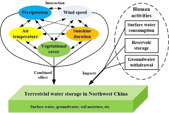
:Monitoring variations in terrestrial water storage (TWS) is of great significance for the management of water resources. However, it remains a challenge to continuously monitor TWS variations using in situ observations and hydrological models because of a limited number of gauge stations and the complicated spatial distribution characteristics of TWS. In contrast, the Gravity Recovery and Climate Experiment (GRACE) could overcome the aforementioned restrictions, providing a new reliable means of observing TWS variation. Thus, GRACE was employed to investigate TWS variations in Northwest China (NWC) between April 2002 and March 2016. Unlike previous studies, we focused on the interactions of multiple climatic and vegetational factors, and their combined effects on TWS variation. In addition, we also analyzed the relationship between TWS variations and socioeconomic water consumption. The results indicated that (i) TWS had obvious seasonal variations in NWC, and showed significant decreasing trends in most parts of NWC at the 95% confidence level; (ii) decreasing sunshine duration and wind speed resulted in an increase in TWS in Qinghai province, whereas the increasing air temperature, ameliorative vegetational coverage, and excessive groundwater withdrawal jointly led to a decrease in TWS in the other provinces of NWC; (iii) TWS variations in NWC had a good correlation with water storage variations in cascade reservoirs of the upper Yellow River; and (iv) the overall interactions between multiple climatic and vegetational factors were obvious, and the strong effects of some climatic and vegetational factors could mask the weak influences of other factors in TWS variations in NWC. Hence, it is necessary to focus on the interactions of multiple factors and their combined effects on TWS variations when exploring the causes of TWS variations.
1. Introduction
Terrestrial water storage (TWS), including surface water, groundwater, snow cover, and soil moisture, not only plays an important role in the global hydrological cycle, but also provides abundant freshwater resources for human society and the terrestrial ecological system [1,2,3]. With a changing environment (climate change and human activities), TWS has obvious variations in many river basins and/or regions, which bring big challenges to local water resource management and utilization [3,4,5]. It is imperative to continually monitor TWS variations. However, it is impossible to do so using in situ observations and hydrological models due to a limited number of gauge stations and the complicated spatial distribution characteristics of TWS [6,7,8]. Accordingly, a more advanced technology is hoped to effectively tackle this tricky issue.
To observe spatial and temporal changes of Earth’s gravity field, the National Aeronautics and Space Administration (NASA) and the German Aerospace Center (DLR) jointly developed the Gravity Recovery and Climate Experiment (GRACE) satellite mission [9]. Since the launch of the GRACE satellite mission in March 2002, an increasing number of hydrologists realized that it could act as a new effective tool for measuring TWS variations. GRACE could continuously measure TWS variations through conversion of the gravitational field, breaking the limitations of spatial heterogeneity for TWS. Furthermore, many recent research results showed that GRACE is able to provide reliable data for an investigation of TWS in a large area on a monthly basis [10,11,12,13,14].
Until now, most studies were concerned with the spatiotemporal characteristics of TWS variations based on GRACE, paying less attention to the causes of TWS variations [3]. To determine the causes of TWS variations, some scholars investigated the relationships between TWS and climatic and vegetational factors. Li et al. [15] found a good correlation between TWS and vegetational coverage in western and central Europe during droughts, on the basis of a severe deficiency in TWS harming vegetational growth to a large extent. Zhou et al. [16] suggested that TWS was dominated by precipitation in the Poyang Lake basin. Deng and Chen [3] showed the effects of precipitation and air temperature on TWS in Central Asia over the past decade. These studies substantially promoted the causal analysis of TWS variations. However, most previous studies only showed a correlation between GRACE-based TWS and one factor on a monthly basis without considering the combined effects and the interactions of multiple factors. This probably generated some unreliable correlations, maybe even misleading the causal analysis of TWS variations. For example, Deng and Chen [3] found that monthly TWS and monthly average air temperature (AT) had an obviously positive correlation in Xinjiang; however, they failed to clearly explain the effect of AT on TWS due to the combined effects of air temperature, precipitation, and wind speed on TWS. In contrast, this study paid more attention to the interactions of multiple factors and their combined effects on TWS variations.
Precipitation (P) and evapotranspiration (Et) directly influence TWS variation; however, it is difficult to access actual Et in a large region. According to the Penman–Monteith equation [17,18], Et is influenced by many climatic factors, such as sunshine duration (SD), air temperature (AT), and wind speed (WS). In addition, vegetational growth also has important effects on Et [19]. The normalized difference vegetation index (NDVI), an index for the greenness of vegetation, could characterize vegetation growth [20]. Thus, multiple climatic and vegetational factors including P, SD, AT, WS, and NDVI were adopted to account for TWS variations in this study.
In addition to climatic and vegetational factors, some studies also analyzed the relationship between TWS variations and socioeconomic water consumption. Rodell et al. [21] suggested that groundwater depletion was mainly attributable to irrigation in northwest India. Feng et al. [22] believed that a decrease in TWS was caused by agricultural water consumption in North China. Moreover, Deng and Chen [3] deemed that agricultural diversion and groundwater withdrawal were primarily attributable to the decrease in TWS in Central Asia. Artificial reservoirs play a significant role in utilizing and managing surface water resources [23]; however, few studies explore the relationship between TWS changes and reservoir operation. In addition to discussing the effects of groundwater withdrawals, this study also briefly analyzed the correlation between water storage variations in reservoirs and TWS variations.
Northwest China (NWC) is a typical arid and semi-arid region playing an important strategic role in the social and economic development of China [24,25,26]. Since the implementation of the Belt and Road initiative of China, this region faces an unprecedented new opportunity for development [27]. With rapid socioeconomic development, the water shortage problem became increasingly severe in NWC. To our knowledge, this study is the first study employing GRACE data to characterize TWS variations in NWC. The results of this study are proposed to hopefully help the management of local water resources in this region.
Two targets were established for this study. The first was to examine TWS variations in NWC, and to identify the relationships between TWS and climate change, vegetational coverage, and socioeconomic water consumption. The second was to show the interactions of multiple climatic and vegetational factors, and their combined effects on TWS variations. The paper is organized as follows: Section 2 describes the study area, data collection and processing, and two correlation analysis methods for hydrological and meteorological time series; Section 3 describes the detailed TWS variations in NWC, and an analysis of relationships between TWS and climate change, vegetational coverage, and socioeconomic water consumption; Section 4 presents the major conclusions of this study.
2. Materials and Methods
2.1. Study Area
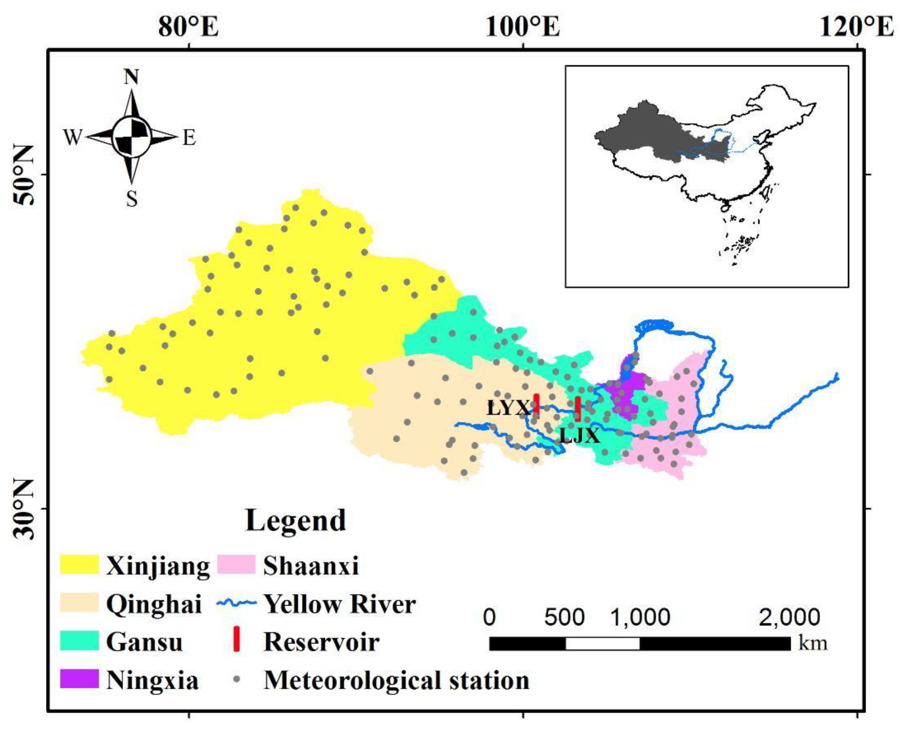
NWC, shown in Figure 1, includes the Shaanxi, Ningxia, Gansu, Qinghai, and Xinjiang provinces. NWC is in the interior of China and is located far from oceans, having a total area of 3.11 million km2. Its terrain is very complex, consisting of mountains, plateaus, basins, and plains. Among the five provinces, the area of Xinjiang (1.66 million km2) is the largest, and the average elevation of Qinghai (3000 m above sea level) is the highest. Most parts of NWC are mainly characterized by an arid or semi-arid climate, and the annual average precipitation in Shaanxi (634 mm) and Xinjiang (144 mm) are the maximum and minimum values, respectively. Overall, the ecosystem of NWC is rather vulnerable, particularly in Xinjiang where 64% of the area is desertified land as of the end of 2014 [28]. The upstream of the Yellow River flows through the Qinghai, Gansu, Ningxia, and Shaanxi provinces. In the upper Yellow River, Longyangxia (LYX) and Liujiaxia (LJX) in the Qinghai and Gansu provinces, respectively, are two large cascade reservoirs with a total storage capability of 30.4 billion m3 [29].
2.2. Data Collection
Three Release-05 gravity-field solutions were obtained separately from three different data processing centers: the University of Texas Center for Space Research (CSR; http://www.csr.utexas.edu/grace/), the German Research Center for Geosciences (GFZ; http://isdc.gfz-potsdam.de/grace), and the Jet Propulsion Laboratory (JPL; http://grace.jpl.nasa.gov/). The differences between the solutions obtained from the JPL, CSR, and GFZ were used to infer the uncertainty in the Level-2 GRACE fields [30]. Three sets of monthly gravity-field time series of NWC were collected from April 2002 to March 2016, a total of 168 months (13 months with missing data). TWS includes surface water, groundwater, snow cover, and soil moisture. Thus, to evaluate the products is challenging because of the unavailability of a reference dataset (field measurements) for each component of TWS in the study region. Nevertheless, numerous studies demonstrated the reliability of these datasets for monitoring the variation in TWS worldwide on monthly, seasonal, and annual bases [21,22,31,32].
Monthly P, SD, AT, and WS data (from January 1982 to March 2016) were collected from 192 meteorological stations (Figure 1) distributed across NWC, which could be downloaded from the National Meteorological Information Center of China (http://data.cma.cn/). Remote sensing data (MOD13C2 product) based on the moderate resolution imaging spectroradiometer (MODIS) sensors aboard the Terra satellite were downloaded from the Land Processes Distributed Active Archive Center (LP DAAC) of the National Aeronautics and Space Administration (https://lpdaac.usgs.gov/). Data on the monthly variation in storage of the LYX and LJX reservoirs (from April 2002 to March 2016) were obtained from the water year books and water-resources bulletins for Yellow River, which were released by the Yellow Conservancy Commission of the Ministry of Water Resources of China (http://www.yellowriver.gov.cn/). In addition, the annual groundwater withdrawal data (from 2002 to 2015) were collected from the water-resources bulletins released by the respective departments (http://www.sxmwr.gov.cn/; http://www.nxsl.gov.cn/; http://www.gssl.gov.cn/; http://www.qhsl.gov.cn/; http://www.xjslt.gov.cn/) of the five provinces in NWC.
2.3. Data Processing
(1) TWS Data Processing
In this study, the average monthly gravity field (between January 2004 and December 2009) was taken as the baseline of the monthly gravity-field time series (from April 2002 to March 2016), i.e., a monthly gravity field anomaly was generated following the subtraction of the baseline from the monthly gravity field. The missing monthly GRACE data between April 2002 and March 2016 were interpolated using the linear interpolation method. To eliminate the influence of noise, a Gauss smoothing kernel [33] was introduced into the calculation of gravity-field anomalies, which was expressed as an equivalent water height by the following equation [34]:
where Δh is the equivalent water height; θ is the colatitude; λ is the longitude; a is the equatorial radius (6378 km); ρave is the mean density of the earth (5517 kg/m3); ρwater is the density of water (1000 kg/m3); n is the degree of decomposition; m is the order; kn is the loading love number of the nth degree; Wn denotes Gauss smoothing kernel related to the nth degree, calculated by the recurrence formula W0 = 1, W1 = (1 + e − 2b)/(1 − e − 2b) − 1/b, Wn+1 = −(2n + 1)/b·Wn + Wn−1, b = ln2/(1 − cos(r/a)); r is the filter radius; ΔCnm and ΔSnm are the gravity spherical harmonic coefficient and normalized Stokes coefficient residuals relative to the baseline, respectively; and Pnm (cos(θ)) is the nth degree and the mth-order fully normalized Legendre function.
In Equation (1), the maximum value of the degree (nmax) and the filter radius (r) were two significant parameters, which were neither too large nor too small. If nmax was greater than 60, a larger error would result in the GRACE data [35]. If nmax was too small, the resolution of the gravity field would decrease. A large r could reduce the noise of the GRACE data; however, it probably resulted in some additional errors when it exceeded a study area [36]. In this study, nmax = 60 and r = 300 km. In addition, the C20 (degree 2, order 0) obtained from GRACE was replaced by the C20 from satellite laser ranging (SLR), because the GRACE-C20 values had a larger uncertainty than those of the SLR-C20 values [37,38].
Monthly variations in land gravity fields are mainly caused by monthly TWS changes [39,40]. Hence, a monthly equivalent water height represents a monthly anomaly in TWS, herein named TWSA. Based on the GRACE data from three centers (CSR, GFZ, and JPL), three sets of monthly TWSA time series (from April 2002 to March 2016) for NWC were available to support this study. Because the accuracy differences between three sets of time series were not clear, the cross-correlation coefficients between them were adopted to calculate the weights of the data from the three centers as follows:
where r(X, Y) is the Pearson correlation coefficient between two time series, X and Y [41]; Xk and Yk denote the kth sample values of X and Y, respectively; Xa and Ya represent the averages of X and Y, respectively; n is the length of the two time series; wi is the data weight of the ith center (CSR, GFZ, and JPL were separately numbered 1, 2, and 3); rij denotes the correlation coefficient between two monthly TWSA time series from the ith and jth centers; TWSA is the weighted TWSA time series; and TWSAi is the monthly TWSA time series from the ith center.
When obtaining monthly TWSA time series, the monthly TWS variation could be calculated as shown below [42].
where ΔTWS(i) is the TWS variation of the ith month, and TWSA(i + 1) is the TWSA of the (i + 1)th month.
(2) Climatic Data Processing
For a province in NWC, its monthly climatic time series (from January 1982 to March 2016) was calculated using the Thiessen polygon method as follows [43]:
where M is the climatic factor (P, SD, AT, and WS) value of a province, l is the total number of meteorological stations in the province, fi denotes the Thiessen polygon area controlled by the ith station, and F is the total area of the province.
Specifically, the procedures of the Thiessen polygon method are described below.
- (i)
- Connect the meteorological stations in NWC with straight lines, creating a Delaunay triangulation.
- (ii)
- Determine three perpendicular bisectors and a circumcenter for each triangle in the Delaunay triangulation, thus forming many polygons which take perpendicular bisectors and/or the outline of NWC as boundaries.
- (iii)
- Each polygon is controlled by one meteorological station, where the measured climatic factor values represent those over the whole polygon.
- (iv)
- Calculate the climatic factor values over a province according to Equation (6).
The Thiessen polygon method assumes that the climatic factors change linearly between two adjacent meteorological stations. The method is widely used in areas where meteorological stations are not uniformly distributed [43].
(3) NDVI Data Processing
The monthly remote sensing data (from January 1982 to March 2016) were adopted from a MOD13C2 product with a spatial resolution of 0.05 degrees. The remote sensing data were translated into NDVI data by means of the ENVI software [44]. The NDVI data of a province in NWC was the weighted mean value of all gridded NDVI data in the province. Specifically, the weight of each grid was equal to the ratio of overlapping area between the grid and the province to the area of province.
2.4. Cross-Wavelet Transformation
The cross-wavelet transformation (CWT) is able to present the correlation between two time series in both time and frequency domains, combined with the wavelet transformation and cross-spectrum analysis [45]. The CWT is often used to explore the correlations between two annual hydrological and climatic time series [46]. In this study, a CWT based on a Morlet wavelet [47] was mainly employed to investigate resonant periods between the monthly TWSA time series and the monthly climatic and vegetational factor time series.
During the CWT process, WnX(L) and WnY(L) separately denoted the continuous wavelet transformations of two time series, X and Y, respectively, where n is the length of two time series, and L is the time lag. The CWT between X and Y is expressed as WnXY(L) = WnX(L)·WnY*(L), where WnY*(L) is the complex conjugation of WnY(L). The power spectrum of the wavelet is defined as |WnXY(L)|, which reflects the correlation degree between X and Y. The Fourier transformation power spectrum (Pk) of red noise was calculated using the following equation [48]:
Here, b is the autoregressive coefficient of order 1 for a red-noise time series, and N denotes the length of the red-noise time series.
Supposing that the expectation spectra of the two time series, X and Y, are PkX and PkY, the distribution of the cross-wavelet power spectrum [49] is expressed as follows:
where σX and σY denote the standard deviations of the two time series, X and Y, respectively; Zν(p) is the confidence level corresponding to the probability p for a probability distribution function by the square root of two χ2 distributions; and ν is the freedom degree.
In Equation (8), if the left-hand value is larger than the upper limit of the power spectrum of red noise under the significance level, α, it is thought that the correlation between X and Y is significant.
2.5. Pearson Correlation Coefficient Test
The Pearson correlation coefficient (PCC) denotes a certain dependency relationship between two time series, X and Y, including the direction and degree of correlation. The PCC in Equation (2) is a traditional and effective statistic for correlation analysis. Its plus/minus sign and absolute value reflect the direction and degree of correlation between two time series, respectively. If X and Y are stationary, a statistic is built as follows [50]:
where t is the statistic following a Student’s t-distribution with a degree of freedom, n − 2; r is the PCC between two time series; and n is the length of the two time series.
When the significance of r is tested, the null hypothesis is that r is equal to zero, i.e., the two time series have no correlation. At the significance level, α, the null hypothesis is rejected if the absolute value of t is larger than tα/2.
In reality, a time series may be non-stationary, which could reduce the effectiveness of the PCC. In addition, the periodic components in both time series probably lead to a false correlation. Thus, the resonant periodic components and their respective trend components are removed from X and Y before analyzing their correlation. Specifically, it is assumed that X and Y have significant resonant periods, and their separate periodic components are XP and YP, respectively. In addition, both X-XP and Y-YP have separate, overall linear trend components, XT and YT, respectively. The PPC between X-XP-XT and Y-YP-YT is r’ with the statistic t’. If |t’| is larger than tα/2, X and Y have a significant correlation depending on r’; otherwise, it is insufficient to determine the correlation between X and Y based on r’.
For brevity, r and r’ were named original PCC and filtered PCC, respectively. It is assumed that m factors (X1, X2, …, Xm) jointly influence a factor (Y). Furthermore, ri (i = 1, 2, …, m) and r’i are the original and filtered PCCs between the Xi and Y time series. According to the (positive or negative) sign of r*·r’i and the value of |r’i|, the effects of different factors (X1, X2, …, Xm) on Y could be ranked. If r*r’j > 0 and r*r’k < 0 (j, k = 1, 2, …, m), the effect of Xj on Y is larger than that of Xk. If r*r’j and r*r’k have the same sign and |r’j| > |r’k|, the effect of Xj on Y is larger than that of Xk; otherwise, the effect of Xj on Y is smaller than that of Xk.
3. Results and Discussion
3.1. Data Weights of the Three Centers
Figure 2 shows the correlations of monthly TWSA time series measured by the three centers (CSR, GFZ, and JPL). All correlation coefficients were greater than 0.7, indicating that the TWSA data of NWC measured by the three centers were highly consistent. The correlation between CSR and GFZ was the highest, while the correlation between GFZ and JPL was the lowest. In addition, the correlations of the three centers decreased from east to west in NWC, which probably resulted from the increase in gravity-field inversion error related to the increases in regional size and topographic complexity in this direction [51]. Based on the correlations, the data weights of the three centers were calculated, and are presented in Table 1, thus obtaining the monthly weighted TWSA time series of NWC.
3.2. TWS Variations in the NWC
Figure 3 shows the intra-annual variations in TWS in the five provinces of NWC. It can be seen that the TWS showed distinct seasonal variations, and TWS variations in Xinjiang province were quite different from those in the other four provinces. In the Shaanxi, Ningxia, Gansu, and Qinghai provinces, TWS increased from April to September, and basically decreased from September to April. In the Xinjiang province, TWS decreased from April to October, and increased from October to April. Yang and Chen [12] found that TWS reached maximum and minimum values in April and October, respectively, in the Central Xinjiang province, which is consistent with the changing characteristics of TWS in the Xinjiang province in this study.
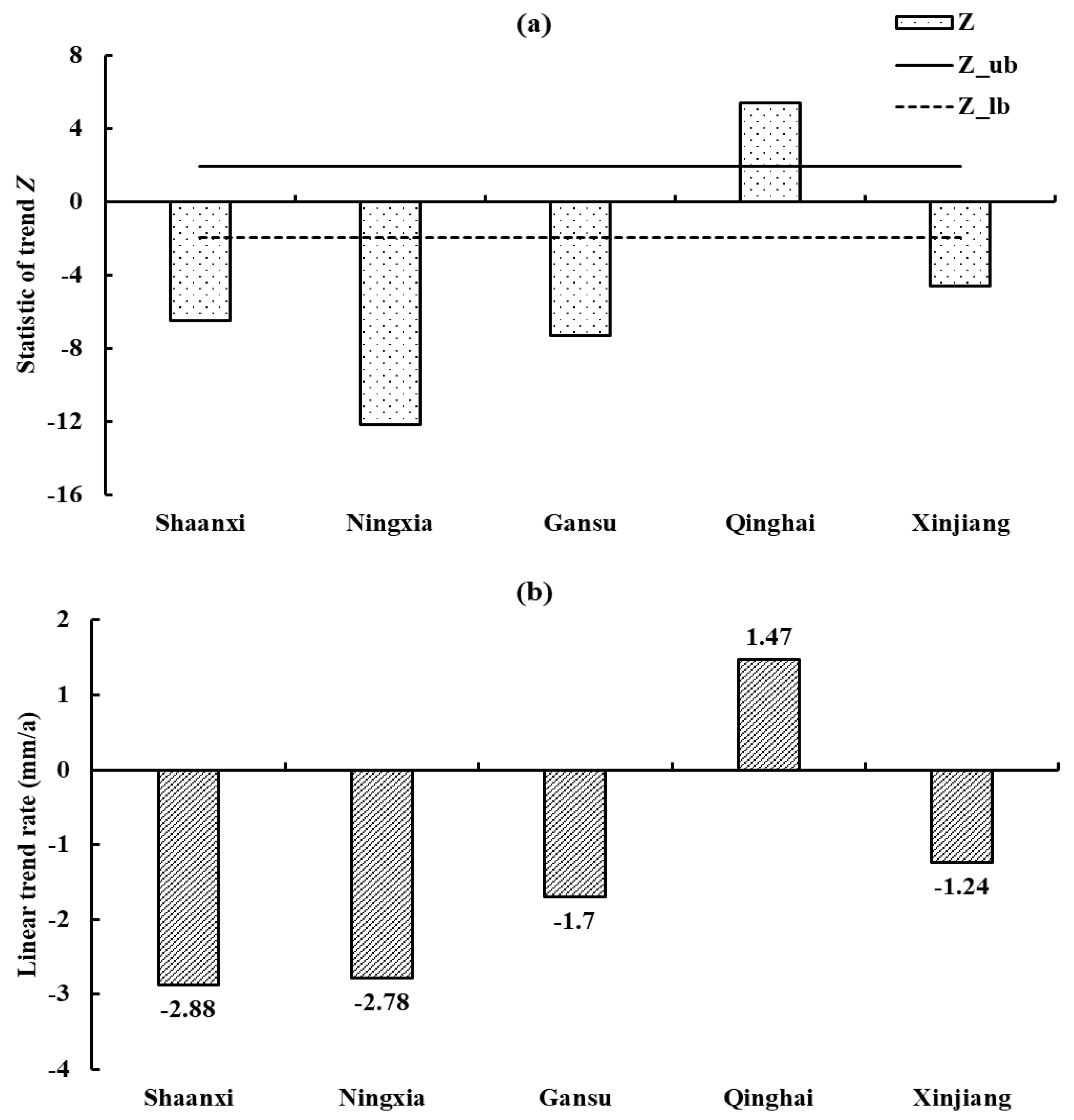
Using a Mann–Kendall test [52], the trends in Figure 4a show that TWS in Qinghai had a significant trend, with an increasing rate of 1.47 mm/a in Figure 4b, while TWS in the other four provinces (Shaanxi, Ningxia, Gansu, and Xinjiang) obviously decreased. Figure 4b shows the linear rates of TWS in the five provinces. Specifically, ranking the rates of TWS decrease from fastest to slowest yields Shaanxi (−2.88 mm/a), Ningxia (−2.78 mm/a), Gansu (−1.7 mm/a), and Xinjiang (−1.24 mm/a). According to the available literature [3,12,53,54,55], TWS had a significant decline in the Xinjiang province, particularly in the Tianshan Mountains and surrounding areas. TWS had an obvious increase at the intersection between Tibet and the Xinjiang and Qinghai provinces. TWS notably decreased in the Shaanxi and Ningxia provinces between 2003 and 2013. In addition, TWS also obviously decreased in the North Gansu province from 2003 to 2012.
3.3. Correlations between TWS and Climatic and Vegetational Factors
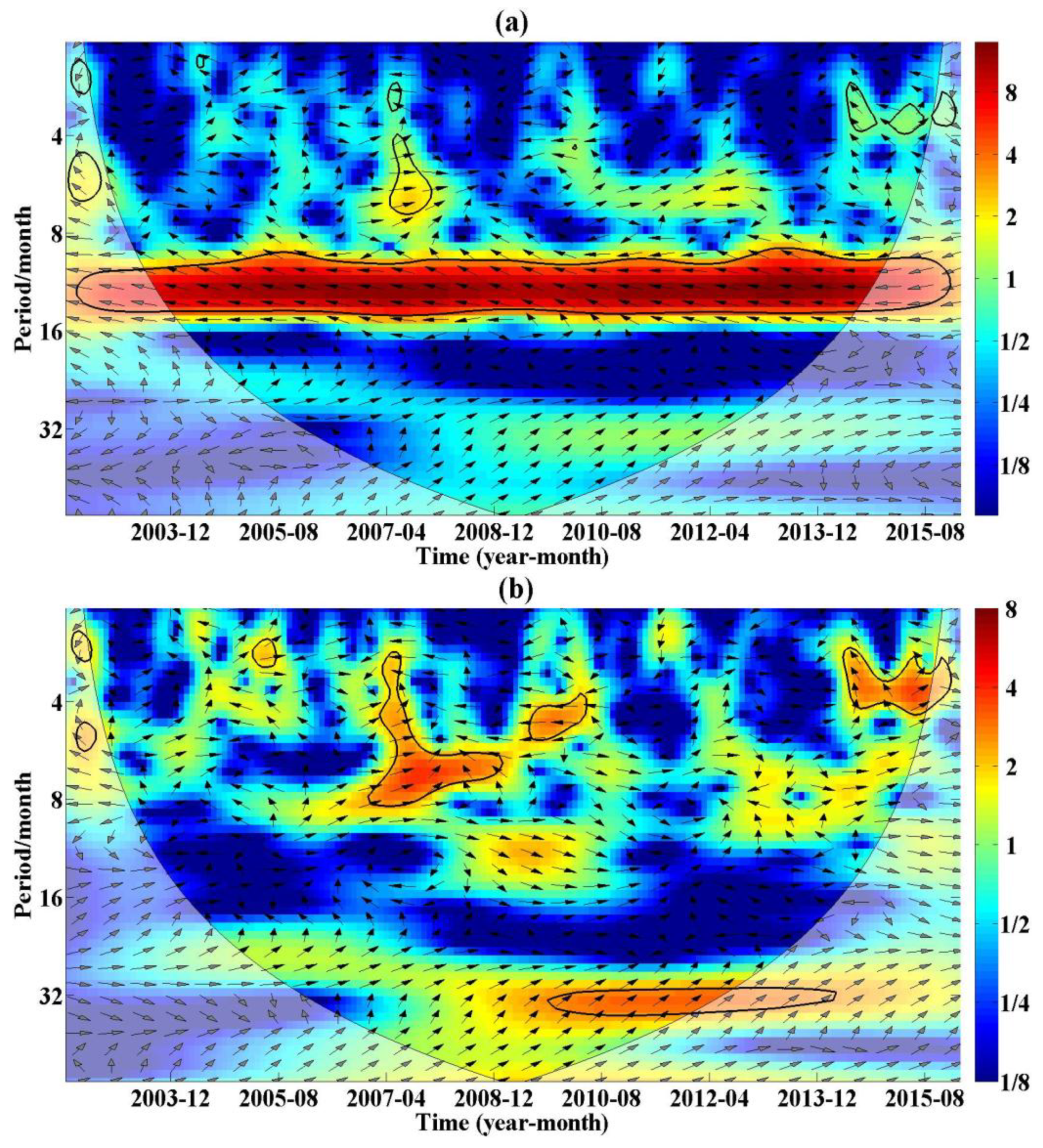
CWT was utilized to analyze the correlations between ΔTWS and climatic and vegetational factors in NWC. For brevity, Figure 5 only shows the CWTs between the monthly ΔTWS and P series in the Xinjiang province of NWC. The main information of the cross-wavelet power spectrum, like that in Figure 5a, could be described as follows: (1) the influencing cone of the wavelet, namely the area surrounded by the fine arc, is set to avoid the boundary effect and the false information outside the cone; (2) the area surrounded by the thick real line denotes the cross-wavelet power spectrum passing the test of standard spectrum of red noise under the significance level, α = 0.05; (3) the numbers on the right of the color bar represent the relative power spectrum values (dimensionless value); (4) darker red corresponding to a bigger spectrum value denotes a more significant resonant period (RP), while darker blue corresponding to a smaller spectrum value indicates a less significant RP; and (5) the arrow represents the phase relationship between factor 1 (such as precipitation) and factor 2 (such as ΔTWS). Specifically, “→” denotes that the variations of factors 2 and 1 are synchronous, “↓” indicates that the variation of factor 2 lags behind that of factor 1 with one-fourth of an RP, “←” implies that the variation of factor 2 lags behind that of factor 1 with half of an RP, and “↑” shows that the variation of factor 2 lags behind that of factor 1 with three-fourths of an RP. Additional information about wavelet cross spectra was given by Herrera et al. [56].
Without eliminating periodic and trend components, as shown in Figure 5a, monthly ΔTWS and P had a significant resonant period of 12 months. The ΔTWS value was negatively correlated with P as a whole, but monthly ΔTWS and P had a positive relationship according to the terrestrial water budget equation. In the Xinjiang province, the multi-year average ratio of P to potential Et was less than 0.1 [57]; thus, the negative correlation between ΔTWS and Et was far stronger than the positive correlation between ΔTWS and P. As shown in Figure 5b, the negative correlation between ΔTWS and P was greatly weakened, while the positive correlation was enhanced after removing their periodic and trend components. In NWC, monthly ΔTWS and climatic and vegetational factors had a significant resonant period of 12 months, based on the CWT analysis. To obtain reliable correlations, it was necessary to reduce the periodic and trend components before analyzing a correlation between the two factors on a monthly basis.
Overall, correlations between the climatic and vegetational factors were noteworthy, as shown in Table 2. In NWC, the negative correlations were significant between monthly P and monthly SD, AT, and NDVI. Monthly SD had significant positive correlations with monthly AT and NDVI. Monthly AT showed significant positive correlations with monthly NDVI. Monthly WS had no stable correlations with the other four factors. In the Shaanxi, Ningxia, Gansu, and Qinghai provinces, monthly WS had negative correlations with monthly P, and showed positive correlations with monthly SD, AT, and NDVI. However, monthly WS showed a significant positive correlation with monthly P and negative correlations with monthly SD, AT, and NDVI in the Xinjiang province. The significant correlations showed strong interactions between these factors, which could disturb the independent effects of some factors on ΔTWS to a certain extent.
Vegetational coverage was influenced by multiple climatic factors, particularly P, SD, and AT [58,59]. On a monthly scale, the increase of P led to the decreases of SD and AT, which hindered the normal growth process of vegetation, although soil moisture was replenished by P. Thus, the negative correlations between monthly P and NDVI were reasonable in the five northwest provinces. Nevertheless, the vegetational coverage conditions generally had a good positive correlation with antecedent P in an area; for example, Gessner et al. [60] found vegetational coverage was sensitive to P anomalies of the previous one to three months in Central Asia.
Wind speed has multiple effects on the transport of water vapor [61,62]. On one hand, wind can transport water vapor away from a region, improving regional Et. On the other hand, wind can also transport abundant water vapor to a region, promoting regional P. Thus, WS usually had complicated relationships with other climatic and vegetational variables because of its multiple effects on the transport of water vapor. In particular, Xinjiang is far from oceans, and its P is mainly supplied by water vapor from the North Atlantic Ocean and the Indian Ocean [63,64]. Thus, a higher WS could result in more water vapor being transported to Xinjiang, which explains the significant positive correlation between P and WS in this region to a certain extent.
Monthly ΔTWS had different correlations with the five climatic and vegetational factors based on the values of r’, as shown in Table 3. In the Shaanxi, Ningxia, Gansu, and Qinghai provinces, monthly ΔTWS had significant positive correlations with P, and presented obvious negative correlations with SD, AT, and NDVI. Monthly ΔTWS had non-significant negative correlations with WS in the Shaanxi, Ningxia, and Gansu provinces; furthermore, monthly ΔTWS showed a significant negative correlation with WS in the Qinghai province. In the four provinces, all PCCs between monthly ΔTWS and monthly SD, AT, WS, and NDVI changed from positive to negative after removing periodic and trend components; however, PCCs between monthly ΔTWS and P remained positive. This indicated that monthly P had the strongest effects on ΔTWS in the four provinces. In the Xinjiang province, monthly ΔTWS showed non-significant positive correlations with monthly P and WS, while having non-significant negative correlations with monthly SD, AT, and NDVI. However, monthly ΔTWS and monthly SD, AT, and NDVI had strong negative correlations in the Xinjiang province according to the values of r, which implied similarly prominent effects of the three factors on ΔTWS in this region.
Strong effects of one factor were also able to disturb the influences of the weaker factors on ΔTWS in NWC. In the Shaanxi, Ningxia, Gansu, and Qinghai provinces, the effects of P completely overshadowed the influences of SD, AT, WS, and NDVI. Conversely, the effect of P was thoroughly overshadowed in the Xinjiang province, where the annual average P (144 mm) was far less than that of the other four provinces Shaanxi (634 mm), Ningxia (275 mm), Gansu (295 mm), and Qinghai (356 mm) from 1982 to 2015. Deng and Chen [3] found that monthly TWS and P had a significant positive correlation in Southern Xinjiang, and showed a negative correlation in Northern Xinjiang. It was noted that the P in Northern Xinjiang obviously exceeded that in Southern Xinjiang [65]. In addition, Deng and Chen [3] found that monthly TWS and AT had significant positive correlations in most parts of Xinjiang, which was probably a result of disturbances in their periodic and trend components.
3.4. Effects of Climate and Vegetation Changes on TWS Variations
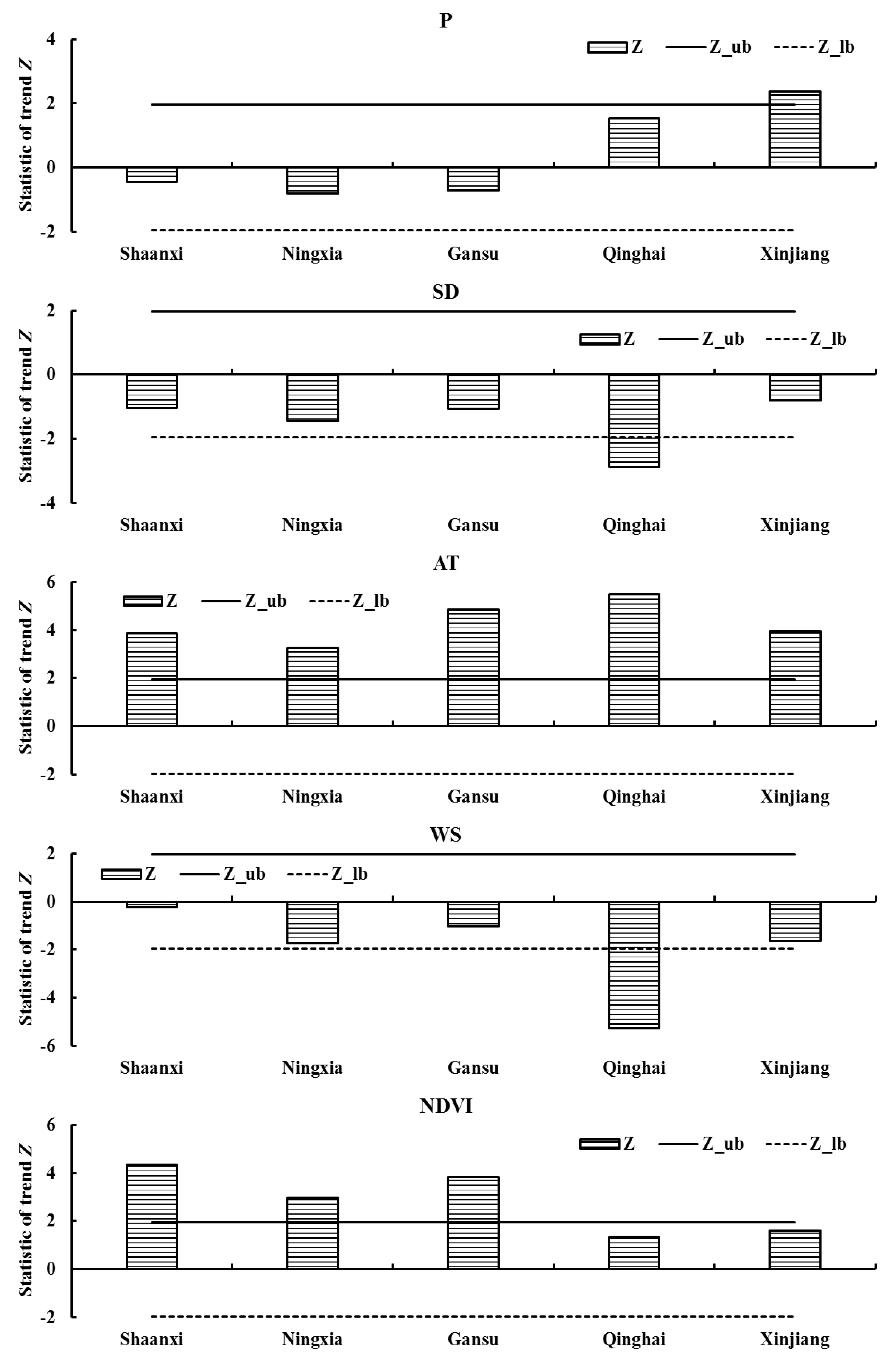
As shown in Figure 6, climatic and vegetational factors had different trends in the five provinces of NWC from 1982 to 2015. Annual AT and NDVI had significant increasing trends in the Shaanxi, Ningxia, and Gansu provinces. Wang et al. [66] also found that vegetation cover had a notable improvement in NWC from 1981 to 2013. Annual SD and WS obviously decreased, while annual AT notably increased in the Qinghai province. Annual P and AT showed significant increasing tendencies in the Xinjiang province, and Deng and Chen [3] detected the same trends of AT and P in the Xinjiang province during recent decades.
Table 4 shows the effects of climatic (P, SD, AT, and WS) and vegetational (NDVI) factors on TWS in the five provinces of NWC. In the Shaanxi, Ningxia, and Gansu provinces, increasing AT and NDVI jointly resulted in decreases in TWS, because the other factors had no significant trends. In the Qinghai province, the decreases in SD and WS jointly caused an increase in TWS, because the increasing AT had a weaker negative influence on TWS than SD and WS. In the Xinjiang province, the increase in AT resulted in a decrease in TWS, because the negative effect of increasing AT was stronger than the positive effect of increasing P.
The significance trends of climatic and vegetational factors changed the hydrological pattern in NWC. In particular, potential evapotranspiration significantly decreased in the western area of NWC because of the decrease in annual WS, while it increased in the eastern area of NWC because of the increase in AT [67]. The increasing AT accelerated the melting of glaciers and snow cover in Xinjiang, leading to a decrease in TWS in the Tianshan Mountains and an increase in TWS in Southern Xinjiang [3,68]. Long-term vegetation restoration reduced soil water storage on the Loess Plateau [69,70]. In addition, vegetation transpiration apparently increased groundwater evapotranspiration in the arid inland river basins of NWC [71].
3.5. Connections between TWS Variations and Socioeconomic Water Consumption
Notably, socioeconomic water consumption (surface water and groundwater consumption) always has direct links with changes in TWS [72]. Based on abundant data on well levels and GRACE-based TWS data, many scholars investigated spatiotemporal variations of regional groundwater [73,74,75,76]. Nevertheless, it is beyond the scope of this study to examine the linkage between the temporal evolution of groundwater storage and groundwater withdrawal, given the challenge of deriving groundwater storage constrained by in situ observations in the study region. This study investigated the relationships between monthly TWS variations and reservoir operation and groundwater withdrawal in NWC.
As shown in Table 5, ΔTWS in the Shaanxi, Ningxia, Gansu, and Qinghai provinces had significant positive correlations with monthly water storage variation in the cascade reservoirs (LYX and LJX) of the upper Yellow River. Thus, the water storage variation of cascade reservoirs could influence ΔTWS in the four provinces. In addition, the correlation coefficients gradually decreased from east to west in NWC. In Figure 7, in addition to Shaanxi, annual water withdrawals from the Yellow River also decreased in this geographical direction. A reasonable explanation was that the downstream water demands influenced the water storage variation of both cascade reservoirs, and further influenced ΔTWS in the three provinces. Though the water withdrawal in Shaanxi was not the largest, the water withdrawals of Gansu and Ningxia probably supply Shaanxi in the form of groundwater, indirectly causing a good correlation between water storage variation in the two cascade reservoirs and ΔTWS in Shaanxi [77].
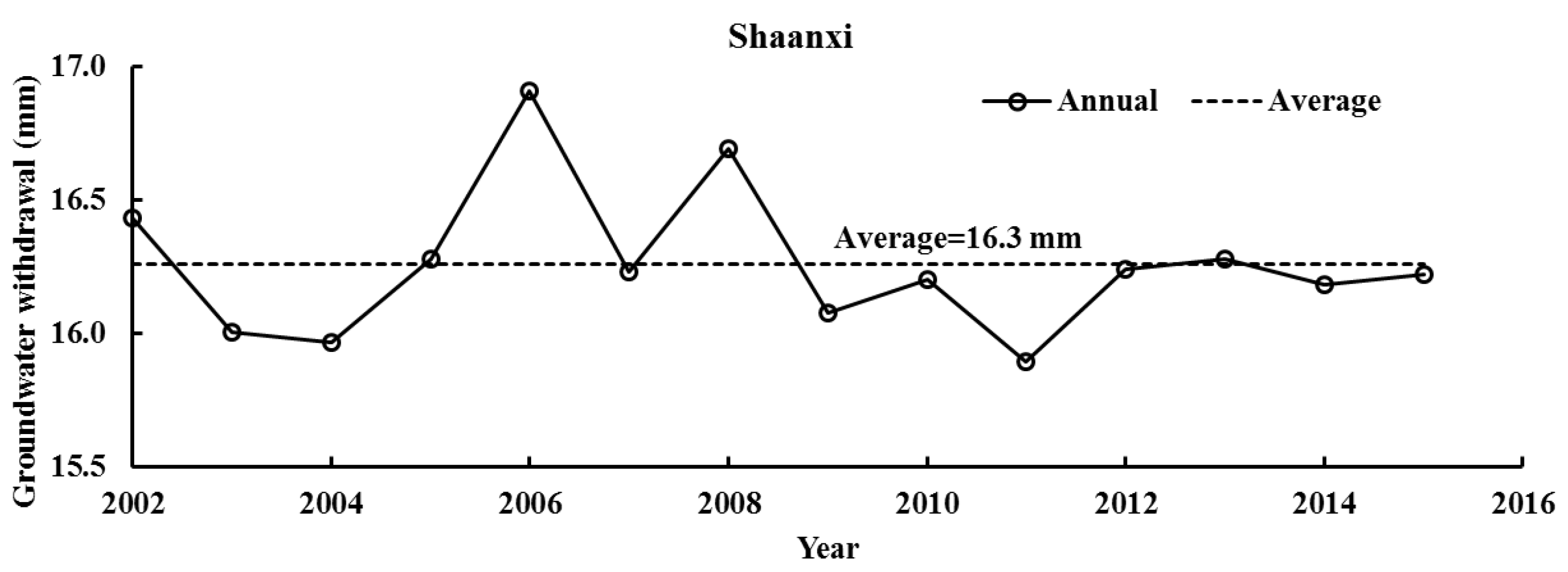
As shown in Figure 8, the annual groundwater withdrawal of Xinjiang province had an obvious increasing trend, while the annual groundwater withdrawals of the other four northwest provinces of NWC had no noticeable trends. Groundwater exploitations are often conducted in the Shaanxi, Ningxia, Gansu, and Xinjiang provinces because of large socioeconomic water demands in these regions [78,79]. As shown in Figure 8, the ranking of the annual average groundwater withdrawals from largest to smallest was Shaanxi (16.3 mm), Ningxia (8.2 mm), Gansu (6.0 mm), Xinjiang (5.0 mm), and Qinghai (0.8 mm), which was consistent with the ranking of decreasing TWS shown in Figure 4b. However, this is not a mere coincidence, as considerable amounts of groundwater are converted into surface water during groundwater withdrawal activities, thereby promoting actual Et and reducing groundwater storage in a province, even under the same climatic and vegetational conditions [80].
In NWC, agricultural irrigation remains the largest source of water usage, accounting for over 70% of total water consumption [79,81]. Irrigation consumes substantial amounts of groundwater every year, leading to severe decreases in groundwater tables in many irrigated farming areas worldwide [82,83]. The groundwater depth gradually increased with the growing number of irrigation wells on the Guanzhong Plain of the Shaanxi province from 1977 to 2010 [84]. The groundwater table significantly declined in the Dunhuang oasis of the Gansu province from 1987 to 2007 because of increased pumping for irrigation [85]. The groundwater levels obviously decreased in the Tarim River basin of the Xinjiang province with the expansion of irrigation between 2004 and 2010 [3]. With increasing AT, irrigation probably consumed more groundwater in some irrigated areas, thus resulting in a further reduction of TWS in NWC.
4. Conclusions
This study investigated GRACE-based TWS variations in NWC between April 2002 and March 2016, including seasonal and trend variations. Furthermore, the relationships between TWS variations and climatic and vegetational factors, as well as socioeconomic water consumption, were analyzed. The major conclusions are as follows:
- (1)
- TWS showed distinct seasonal variations and a significant decreasing tendency in NWC as a whole. In particular, TWS obviously decreased in the Shaanxi, Ningxia, Gansu, and Xinjiang provinces, while TWS notably increased in the Qinghai province. Increases in AT and NDVI were the main causes of the decreases in TWS in the Shaanxi, Ningxia, and Gansu provinces. The decreases in SD and WS resulted in an increase in TWS in the Qinghai province, while the decrease in TWS was caused by the obvious increase in AT in the Xinjiang province.
- (2)
- The interactions of climatic and vegetational factors were significant, and strong effects of some factors could weaken the influences of other factors on TWS variations in NWC. In particular, the negative effects of SD, AT, and NDVI jointly masked the positive effects of P and WS on TWS in the Xinjiang province, whereas the positive effect of P masked the negative effects of the other factors on TWS in the other provinces in NWC. Accordingly, we should emphasize the analysis of the interactions and combined effects of multiple effects on TWS variations in a region.
- (3)
- TWS in the Shaanxi, Ningxia, Gansu, and Qinghai provinces had good correlations with the variation in water storage in the cascade reservoirs of the upstream of the Yellow River, and the correlation coefficients gradually decreased from east to west in NWC. In addition, increasing AT could promote actual Et when more groundwater is converted into surface water in irrigated areas, thus resulting in a further reduction in TWS in NWC.
Author Contributions
Y.X. and S.H. conceived and designed the methodological approach; S.L., G.L., J.P., Q.H. and P.L. undertook the hydrometeorological data, remote sensing data, NDVI data, reservoir storage data, and water withdrawal data collections, respectively. Y.X. carried out the calculation work and analyzed the results, and then wrote the paper. All authors contributed to the revision of the drafts.
Funding
This research was supported by the National Key R&D Program of China (2017YFC0405900), the National Natural Science Foundation of China (51709221), the Planning Project of Science and Technology of Water Resources of Shaanxi (2015slkj-27, 2017slkj-19), and the Key laboratory research projects of education department of the Shaanxi province (17JS104).
Acknowledgments
We are grateful for the Yellow Conservancy Commission of the Ministry of Water Resources and the Water Resources Departments of the five northwest provinces in China providing data for this study. Moreover, sincere gratitude is expanded to the editor and the anonymous reviewers who provided professional comments for this paper.
Conflicts of Interest
The authors declare no conflict of interest.
References
- Famiglietti, J.S. Remote sensing of terrestrial water storage, soil moisture and surface waters. State Planet Front. Chall. Geophys. 2004, 150, 197–207. [Google Scholar]
- Tangdamrongsub, N.; Steele-Dunne, S.C.; Gunter, B.C.; Ditmar, P.G.; Weerts, A.H. Data assimilation of GRACE terrestrial water storage estimates into a regional hydrological model of the Rhine River basin. Hydrol. Earth Syst. Sci. 2015, 19, 2079–2100. [Google Scholar] [CrossRef] [Green Version]
- Deng, H.; Chen, Y. Influences of recent climate change and human activities on water storage variations in Central Asia. J. Hydrol. 2017, 544, 46–57. [Google Scholar] [CrossRef]
- Bhatti, A.M.; Koike, T.; Shrestha, M. Climate change impact assessment on mountain snow hydrology by water and energy budget—Based distributed hydrological model. J. Hydrol. 2016, 543, 523–541. [Google Scholar] [CrossRef]
- Jakob, D.; Walland, D. Variability and long-term change in Australian temperature and precipitation extremes. Weather Clim. Extremes 2016, 14, 36–55. [Google Scholar] [CrossRef]
- Frappart, F.; Seoane, L.; Ramillien, G. Validation of GRACE-derived terrestrial water storage from a regional approach over South America. Remote Sens. Environ. 2013, 137, 69–83. [Google Scholar] [CrossRef] [Green Version]
- Hassan, A.; Jin, S. Water storage changes and balances in Africa observed by GRACE and hydrologic models. Geod. Geodyn. 2016, 7, 39–49. [Google Scholar] [CrossRef]
- Huang, P.; Li, Z.; Chen, J.; Li, Q.; Yao, C. Event-based hydrological modeling for detecting dominant hydrological process and suitable model strategy for semi-arid catchments. J. Hydrol. 2016, 542, 292–303. [Google Scholar] [CrossRef]
- Ramillien, G.; Frappart, F.; Cazenave, A.; Güntner, A. Time variations of land water storage from an inversion of 2 years of GRACE geoids. Earth Planet. Sci. Lett. 2005, 235, 283–301. [Google Scholar] [CrossRef] [Green Version]
- Lenk, O. Satellite based estimates of terrestrial water storage variations in Turkey. J. Geodyn. 2013, 67, 106–110. [Google Scholar] [CrossRef]
- Forootan, E.; Rietbroek, R.; Kusche, J.; Sharifi, M.A.; Awang, J.; Schmidt, M.; Omondi, P.; Famiglietti, J. Separation of large scale water storage patterns over Iran using GRACE, altimetry and hydrological data. Remote Sens. Environ. 2014, 140, 580–595. [Google Scholar] [CrossRef] [Green Version]
- Yang, P.; Chen, Y. An analysis of terrestrial water storage variations from GRACE and GLDAS: The Tianshan Mountains and its adjacent areas, central Asia. Quat. Int. 2015, 358, 106–112. [Google Scholar] [CrossRef]
- Seyoum, W.M.; Milewski, A.M. Monitoring and comparison of terrestrial water storage changes in the northern high plains using GRACE and in-situ based integrated hydrologic model estimates. Adv. Water Resour. 2016, 94, 31–44. [Google Scholar] [CrossRef]
- Abiy, A.Z.; Melesse, A.M. Evaluation of watershed scale changes in groundwater and soil moisture storage with the application of GRACE satellite imagery data. Catena 2017, 153, 50–60. [Google Scholar] [CrossRef]
- Li, B.; Rodell, M.; Zaitchik, B.F.; Reichle, R.H.; Koster, R.D.; van Dam, T.M. Assimilation of GRACE terrestrial water storage into a land surface model: Evaluation and potential value for drought monitoring in western and central Europe. J. Hydrol. 2012, 446–447, 103–115. [Google Scholar] [CrossRef]
- Zhou, Y.; Jin, S.; Tenzer, R.; Feng, J. Water storage variations in the Poyang Lake Basin estimated from GRACE and satellite altimetry. Geod. Geodyn. 2016, 7, 108–116. [Google Scholar] [CrossRef]
- Monteith, J.L. Evaporation and environment. Symp. Soc. Exp. Biol. 1965, 19, 205–234. [Google Scholar] [PubMed]
- Fang, W.; Huang, S.Z.; Huang, Q.; Huang, G.H.; Meng, E.H.; Luan, J.K. Reference evapotranspiration forecasting based on local meteorological and global climate information screened by partial mutual information. J. Hydrol. 2018, 561, 764–779. [Google Scholar] [CrossRef]
- Wang, Y.L.; Wang, X.; Zheng, Q.Y.; Li, C.H.; Guo, X.J. A comparative study on hourly real evapotranspiration and potential evapotranspiration during different vegetation growth stages in the Zoige Wetland. Procedia Environ. Sci. 2012, 13, 1585–1594. [Google Scholar] [CrossRef]
- Tucker, C.J. Red and photographic infrared linear combinations for monitoring vegetation. Remote Sens. Environ. 1979, 8, 127–150. [Google Scholar] [CrossRef] [Green Version]
- Rodell, M.; Velicogna, I.; Famiglietti, J.S. Satellite-based estimates of groundwater depletion in India. Nature 2009, 460, 999–1002. [Google Scholar] [CrossRef] [PubMed] [Green Version]
- Feng, W.; Zhong, M.; Lemoine, J.M.; Biancale, R.; Hsu, H.T.; Xia, J. Evaluation of groundwater depletion in North China using the Gravity Recovery and Climate Experiment (GRACE) data and ground-based measurements. Water Resour. Res. 2013, 49, 2110–2118. [Google Scholar] [CrossRef] [Green Version]
- Haddad, O.B.; Moravej, M.; Loáiciga, H.A. Application of the water cycle algorithm to the optimal operation of reservoir systems. J. Irrig. Drain. Eng. 2014, 141, 04014064. [Google Scholar] [CrossRef]
- Huang, S.Z.; Chang, J.X.; Huang, Q.; Chen, Y.T. Spatio-temporal changes and frequency analysis of drought in the Wei River Basin, China. Water Resour. Manag. 2014, 28, 3095–3110. [Google Scholar] [CrossRef]
- Huang, S.Z.; Chang, J.X.; Huang, Q.; Chen, Y.T. Monthly streamflow prediction using modified EMD-based support vector machine. J. Hydrol. 2014, 511, 764–775. [Google Scholar] [CrossRef]
- Huang, S.Z.; Huang, Q.; Chang, J.X.; Leng, G.Y. Linkages between hydrological drought, climate indices and human activities: A case study in the Columbia River basin. Int. J. Climatol. 2016, 36, 280–290. [Google Scholar] [CrossRef]
- Huang, Y. Understanding China’s Belt and Road Initiative: Motivation, framework and assessment. China Econ. Rev. 2016, 40, 314–321. [Google Scholar] [CrossRef]
- Pan, C.J. Status and management of land desertification in Xinjiang Province. Mod. Hortic. 2018, 41, 179–180. (In Chinese) [Google Scholar]
- Fang, W.; Huang, Q.; Huang, S.Z.; Yang, J.; Meng, E.H.; Li, Y.Y. Optimal sizing of utility-scale photovoltaic power generation complementarily operating with hydropower: A case study of the world’s largest hydro-photovoltaic plant. Energy Convers. Manag. 2017, 136, 161–172. [Google Scholar] [CrossRef]
- Sakumura, C.; Bettadpur, S.; Bruinsma, S. Ensemble prediction and intercomparison analysis of GRACE time-variable gravity field models. Geophys. Res. Lett. 2014, 41, 1389–1397. [Google Scholar] [CrossRef] [Green Version]
- Famiglietti, J.; Lo, M.; Ho, S.; Bethune, J.; Anderson, K.; Syed, T.; Swenson, S.; de Linage, C.; Rodell, M. Satellites measure recent rates of groundwater depletion in California’s Central Valley. Geophys. Res. Lett. 2011, 38, L03403–L03406. [Google Scholar] [CrossRef]
- Scanlon, B.R.; Faunt, C.C.; Longuevergne, L.; Reedy, R.C.; Alley, W.M.; McGuire, V.L.; McMahon, P.B. Groundwater depletion and sustainability of irrigation in the US High Plains and Central Valley. Proc. Natl. Acad. Sci. USA 2012, 109, 9320–9325. [Google Scholar] [CrossRef] [PubMed] [Green Version]
- Swenson, S.; Wahr, J. Methods for inferring regional surface-mass anomalies from Gravity Recovery and Climate Experiment (GRACE) measurements of time-variable gravity. J. Geophys. Res. Atmos. 2002, 107, 389–392. [Google Scholar] [CrossRef]
- Wahr, J.; Molenaar, M.; Bryan, F. Time variability of the Earth’s gravity field: Hydrological and oceanic effects and their possible detection using GRACE. J. Geophys. Res. Solid Earth 1998, 103, 30205–30229. [Google Scholar] [CrossRef]
- Chen, J.L.; Rodell, M.; Wilson, C.R.; Famiglietti, J.S. Low degree spherical harmonic influences on Gravity Recovery and Climate Experiment (GRACE) water storage estimates. Geophys. Res. Lett. 2005, 32, 57–76. [Google Scholar] [CrossRef]
- Werth, S.; Güntner, A.; Schmidt, R.; Kusche, J. Evaluation of GRACE filter tools from a hydrological perspective. Geophys. J. R. Astron. Soc. 2010, 179, 1499–1515. [Google Scholar] [CrossRef]
- Chen, J.L.; Wilson, C.R.; Tapley, B.D.; Ries, J.C. Low degree gravitational changes from GRACE: Validation and interpretation. Geophys. Res. Lett. 2004, 31, 359–393. [Google Scholar] [CrossRef]
- Cheng, M.; Tapley, B.D. Variations in the Earth’s oblateness during the past 28 years. J. Geophys. Res. Solid Earth 2005, 110. [Google Scholar] [CrossRef]
- Tapley, B.D.; Bettadpur, S.; Ries, J.C.; Thompson, P.F.; Watkins, M.M. GRACE measurements of mass variability in the Earth system. Science 2004, 305, 503. [Google Scholar] [CrossRef] [PubMed]
- Chen, J.L.; Wilson, C.R.; Tapley, B.D.; Yang, Z.L.; Niu, G.Y. 2005 drought event in the Amazon River basin as measured by GRACE and estimated by climate models. J. Geophys. Res. Atmos. 2009, 114, B05404. [Google Scholar] [CrossRef]
- Zhou, H.; Deng, Z.; Xia, Y.; Fu, M. A new sampling method in particle filter based on Pearson correlation coefficient. Neurocomputing 2016, 216, 208–215. [Google Scholar] [CrossRef]
- Ramillien, G.; Frappart, F.; Güntner, A.; Ngo-Duc, T.; Cazenave, A.; Laval, K. Time variations of the regional evapotranspiration rate from Gravity Recovery and Climate Experiment (GRACE) satellite gravimetry. Water Resour. Res. 2006, 42, 10403. [Google Scholar] [CrossRef]
- Croley, T.E., II; Hartmann, H.C. Resolving Thiessen polygons. J. Hydrol. 1985, 76, 363–379. [Google Scholar] [CrossRef]
- Bai, J.J.; Bai, J.T.; Wang, L. Spatio-temporal change of vegetation NDVI and its relations with regional climate in Northern Shannxi Province in 2000–2010. Sci. Geogr. Sin. 2014, 34, 882–888. (In Chinese) [Google Scholar]
- Hudgins, L.; Huang, J.P. Bivariate Wavelet Analysis of Asia Monsoon and ENSO. Adv. Atmos. Sci. 1996, 13, 299–312. [Google Scholar] [CrossRef]
- Huang, S.; Huang, Q.; Leng, G.; Meng, E.H. Variations in annual water-energy balance and their correlations with vegetation and soil moisture dynamics: A case study in the Wei River Basin, China. J. Hydrol. 2017, 546, 515–525. [Google Scholar] [CrossRef]
- Niu, J.; Sivakumar, B. Scale-dependent synthetic streamflow generation using a continuous wavelet transform. J. Hydrol. 2013, 496, 71–78. [Google Scholar] [CrossRef]
- Torrence, C.; Compo, G.P. A practical guide to wavelet analysis. Bull. Am. Meteorol. Soc. 1998, 79, 61–78. [Google Scholar] [CrossRef]
- Grinsted, A.; Moore, J.C.; Jevrejeva, S. Application of the cross wavelet transform and wavelet coherence to geophysical time series. Nonlinear Process. Geophys. 2004, 11, 561–566. [Google Scholar] [CrossRef] [Green Version]
- Ndehedehe, C.E.; Agutu, N.O.; Okwuashi, O.; Ferreira, V.G. Spatio-temporal variability of droughts and terrestrial water storage over Lake Chad Basin using independent component analysis. J. Hydrol. 2016, 540, 106–128. [Google Scholar] [CrossRef] [Green Version]
- Luo, Z.; Chen, Y.; Ning, J. Effect of Terrain on the Determination of High Precise Local Gravimetric Geoid. Edit. Board Geomat. Inf. Sci. Wuhan Univ. 2003, 28, 340–344. (In Chinese) [Google Scholar]
- Huang, S.; Hou, B.; Chang, J.; Huang, Q.; Chen, Y. Spatial-temporal change in precipitation patterns based on the cloud model across the Wei River Basin, China. Theor. Appl. Climatol. 2015, 120, 391–401. [Google Scholar] [CrossRef]
- Kang, K.; Li, H.; Peng, P.; Zou, Z. Low-frequency variability of terrestrial water budget in China using GRACE satellite measurements from 2003 to 2010. Geod. Geodyn. 2015, 6, 444–452. [Google Scholar] [CrossRef]
- Yin, W.J.; Hu, L.T.; Wang, J.R. Changes of groundwater storage variation based on GRACE data at the Beishan area, Gansu province. Hydrogeol. Eng. Geol. 2015, 42, 29–34. (In Chinese) [Google Scholar]
- Zhao, Q.; Wu, W.; Wu, Y. Variations in China’s terrestrial water storage over the past decade using GRACE data. Geod. Geodyn. 2015, 6, 187–193. [Google Scholar] [CrossRef]
- Herrera, V.M.V.; Soon, W.; Herrera, G.V.; Traversi, R.; Horiuchi, K. Generalization of the cross-wavelet function. New Astron. 2017, 56, 86–93. [Google Scholar] [CrossRef]
- Li, Y.; Sun, C. Impacts of the superimposed climate trends on droughts over 1961–2013 in Xinjiang, China. Theor. Appl. Climatol. 2016, 129, 977–994. [Google Scholar] [CrossRef]
- Xu, W.; Gu, S.; Zhao, X.Q.; Xiao, J.S.; Tang, Y.H.; Fang, J.Y.; Zhang, J.; Jiang, S. High positive correlation between soil temperature and NDVI from 1982 to 2006 in alpine meadow of the Three-River Source Region on the Qinghai-Tibetan Plateau. Int. J. Appl. Earth Observ. Geoinf. 2011, 13, 528–535. [Google Scholar] [CrossRef]
- Kong, D.; Zhang, Q.; Singh, V.P.; Shi, P. Seasonal vegetation response to climate change in the northern hemisphere (1982–2013). Glob. Planet. Chang. 2017, 148, 1–8. [Google Scholar] [CrossRef]
- Gessner, U.; Naeimi, V.; Klein, I.; Kuenzer, C.; Klein, D.; Dech, S. The relationship between precipitation anomalies and satellite-derived vegetation activity in Central Asia. Glob. Planet. Chang. 2013, 110, 74–87. [Google Scholar] [CrossRef]
- Mcvicar, T.R.; Roderick, M.L.; Donohue, R.J.; Li, L.T.; Niel, T.G.V.; Thomas, A.; Grieser, J.; Jhajharia, D.; Himri, Y.; Mahowald, N.M.; et al. Global review and synthesis of trends in observed terrestrial near-surface wind speeds: Implications for evaporation. J. Hydrol. 2012, 416, 182–205. [Google Scholar] [CrossRef]
- Kousari, M.R.; Ahani, H.; Hakimelahi, H. An investigation of near surface wind speed trends in arid and semiarid regions of Iran. Theor. Appl. Climatol. 2013, 114, 153–168. [Google Scholar] [CrossRef]
- Dai, X.G.; Wang, P.; Zhang, K.J. A study on precipitation trend and fluctuation mechanism in northwestern China over the past 60 years. Acta Phys. Sin. 2013, 62, 129201. [Google Scholar] [CrossRef]
- Huang, W.; Chang, S.Q.; Xie, C.L.; Zhang, Z.P. Moisture sources of extreme summer precipitation events in North Xinjiang and their relationship with atmospheric circulation. Adv. Clim. Chang. Res. 2017, 8, 12–17. [Google Scholar] [CrossRef]
- Zhu, X.; Zhang, M.; Wang, S.; Qiang, F.; Zeng, T.; Ren, Z.; Dong, L. Comparison of monthly precipitation derived from high-resolution gridded datasets in arid Xinjiang, central Asia. Quat. Int. 2015, 358, 160–170. [Google Scholar] [CrossRef]
- Wang, W.; Feng, Q.S.; Guo, N.; Sha, S.; Hu, D.; Wang, L.J.; Li, Y.H. Dynamic monitoring of vegetation coverage based on long time-series NDVI data sets in northwest arid region of China. Pratac. Sci. 2015, 32, 1969–1979. (In Chinese) [Google Scholar]
- Yin, Y.H.; Wu, S.H.; Dai, E.F. Determining factors in potential evapotranspiration changes over China in the period 1971–2008. Sci. Bull. 2010, 55, 3329–3337. [Google Scholar] [CrossRef]
- Tang, X.L.; Lv, X.; He, Y. Features of climate change and their effects on glacier snow melting in Xinjiang, China. C. R. Geosci. 2013, 345, 93–100. [Google Scholar] [CrossRef]
- Yang, L.; Wei, W.; Chen, L.; Chen, W.; Wang, J. Response of temporal variation of soil moisture to vegetation restoration in semi-arid Loess Plateau, China. Catena 2014, 115, 123–133. [Google Scholar] [CrossRef] [Green Version]
- Zhang, Y.W.; Deng, L.; Yan, W.M.; Shangguan, Z.P. Interaction of soil water storage dynamics and long-term natural vegetation succession on the Loess Plateau, China. Catena 2016, 137, 52–60. [Google Scholar] [CrossRef]
- Shen, Q.; Gao, G.; Fu, B.; Lü, Y. Responses of shelterbelt stand transpiration to drought and groundwater variations in an arid inland river basin of Northwest China. J. Hydrol. 2015, 531, 738–748. [Google Scholar] [CrossRef] [Green Version]
- Döll, P.; Dobrev, H.H.; Portmann, F.T.; Siebert, S.; Eicker, A.; Rodell, M.; Strassberg, G.; Scanlon, B.R. Impact of water withdrawals from groundwater and surface water on continental water storage variations. J. Geodyn. 2012, 59–60, 143–156. [Google Scholar] [CrossRef]
- Yeh, J.F.; Swenson, S.C.; Famiglietti, J.S.; Rodell, M. Remote sensing of groundwater storage changes in Illinois using the Gravity Recovery and Climate Experiment (GRACE). Water Resour. Res. 2006, 42, 395–397. [Google Scholar] [CrossRef]
- Scanlon, B.R.; Longuevergne, L.; Long, D. Ground referencing GRACE satellite estimates of groundwater storage changes in the California Central Valley, USA. Water Resour. Res. 2012, 48, 4520. [Google Scholar] [CrossRef]
- Döll, P.; Schmied, H.M.; Schuh, C.; Portmann, F.T.; Eicker, A. Global-scale assessment of groundwater depletion and related groundwater abstractions: Combining hydrological modeling with information from well observations and GRACE satellites. Water Resour. Res. 2015, 50, 5698–5720. [Google Scholar] [CrossRef]
- Bhanja, S.N.; Mukherjee, A.; Saha, D.; Velicogna, I.; Famiglietti, J.S. Validation of GRACE based groundwater storage anomaly using in-situ groundwater level measurements in India. J. Hydrol. 2016, 2016, 543. [Google Scholar] [CrossRef]
- Cui, Y.L.; Zhang, G.; Shao, J.L. Classification and Characteristics of Groundwater System in the Yellow River Basin. Resour. Sci. 2004, 26, 2–8. (In Chinese) [Google Scholar]
- Jing, J.; Sun, J.; Han, S.; Wang, S. Distribution of groundwater resources and the state of development and utilization in the northwestern area. South-to-North Water Transf. Water Sci. Technol. 2007, 5, 54–56. (In Chinese) [Google Scholar]
- Liu, X.; Shen, Y.; Guo, Y.; Li, S.; Guo, B. Modeling demand/supply of water resources in the arid region of northwestern China during the late 1980s to 2010. J. Geogr. Sci. 2015, 25, 573–591. [Google Scholar] [CrossRef]
- Hu, X.; Shi, L.; Zeng, J.; Yang, J.; Zha, Y.; Yao, Y.; Cao, G. Estimation of actual irrigation amount and its impact on groundwater depletion: A case study in the Hebei Plain, China. J. Hydrol. 2016, 543, 433–449. [Google Scholar] [CrossRef]
- Leng, G.; Tang, Q. Modeling the impacts of future climate change on irrigation over China: Sensitivity to adjusted projections. J. Hydrometeorol. 2014, 15, 2085–2103. [Google Scholar] [CrossRef]
- Leng, G.; Huang, M.; Tang, Q.; Gao, H.; Leung, L. Modeling the effects of groundwater-fed irrigation on terrestrial hydrology over the conterminous United States. J. Hydrometeorol. 2014, 15, 957–972. [Google Scholar] [CrossRef]
- Leng, G.; Huang, M.; Tang, Q.; Leung, L. A modeling study of irrigation effects on global surface water and groundwater resources under a changing climate. J. Adv. Model. Earth Syst. 2015, 7, 1285–1304. [Google Scholar] [CrossRef] [Green Version]
- Li, P.; Wei, X.; Jiang, Y.; Feng, D. Response of groundwater cycle to environmental changes in Guanzhong Plain irrigation district. Trans. Chin. Soc. Agric. Eng. 2014, 30, 123–131. (In Chinese) [Google Scholar]
- Zhang, X.; Zhang, L.; He, C.; Li, J.; Jiang, Y.; Ma, L. Quantifying the impacts of land use/land cover change on groundwater depletion in Northwestern China-A case study of the Dunhuang oasis. Agric. Water Manag. 2014, 146, 270–279. [Google Scholar] [CrossRef]
Figure 1.
Location of Northwest China (NWC), including meteorological stations and cascade reservoirs in the upstream of the Yellow River.
Figure 1.
Location of Northwest China (NWC), including meteorological stations and cascade reservoirs in the upstream of the Yellow River.

Figure 2.
Correlation coefficients between monthly time series of terrestrial water storage anomalies (TWSA) of NWC measured by three data centers from April 2002 to March 2016. CSR—the University of Texas Center for Space Research; GFZ—the German Research Center for Geosciences; JPL—the Jet Propulsion Laboratory.

Figure 3.
Multi-year averages of monthly TWS in the five provinces in NWC between April 2002 and March 2016.
Figure 3.
Multi-year averages of monthly TWS in the five provinces in NWC between April 2002 and March 2016.

Figure 4.
Trends of monthly TWSA time series in NWC from April 2002 to March 2016: (a) significance test results of the overall trends; Z is the statistic of the trend of a time series, and Z_ub and Z_lb separately denote the upper and lower bounds of non-significant trends under the significance level, α = 0.05; (b) linear trend rates of TWS in the five provinces of NWC.

Figure 5.
Cross-wavelet transformations (CWTs) between time series of the variations in TWS (ΔTWS) and precipitation (P) in Xinjiang from May 2002 to February 2016: (a) Original ΔTWS and P time series; (b) ΔTWS and P time series with periodic components and linear trend components removed.
Figure 5.
Cross-wavelet transformations (CWTs) between time series of the variations in TWS (ΔTWS) and precipitation (P) in Xinjiang from May 2002 to February 2016: (a) Original ΔTWS and P time series; (b) ΔTWS and P time series with periodic components and linear trend components removed.

Figure 6.
Significance tests of the trends of annual climatic (precipitation (P), sunshine duration (SD), air temperature (AT), and wind speed (WS)) and vegetational (normalized difference vegetation index (NDVI)) factor time series in NWC from 1982 to 2015. (Z is the statistic of the trend of a time series, and Z_ub and Z_lb separately denote the upper and lower bounds of non-significant trends under the significance level, α = 0.05.).

Figure 7.
Annual water withdrawals of the four provinces from the Yellow River between 2002 and 2015.
Figure 7.
Annual water withdrawals of the four provinces from the Yellow River between 2002 and 2015.

Figure 8.
Annual groundwater withdrawals of the five provinces in NWC.


Table 1.
Weights of monthly the Gravity Recovery and Climate Experiment (GRACE) data released by the three centers from April 2002 to March 2016.
Table 1.
Weights of monthly the Gravity Recovery and Climate Experiment (GRACE) data released by the three centers from April 2002 to March 2016.
| Province | CSR | GFZ | JPL |
|---|---|---|---|
| Shaanxi | 0.335 | 0.333 | 0.333 |
| Ningxia | 0.335 | 0.334 | 0.331 |
| Gansu | 0.337 | 0.332 | 0.331 |
| Qinghai | 0.341 | 0.332 | 0.327 |
| Xinjiang | 0.344 | 0.331 | 0.326 |
Note: CSR denotes the University of Texas Center for Space Research; GFZ denotes the German Research Center for Geosciences; and JPL denotes the Jet Propulsion Laboratory.
Table 2.
Pearson correlation coefficients (PCCs) between monthly climatic (precipitation (P), sunshine duration (SD), air temperature (AT), and wind speed (WS)) and vegetational (normalized difference vegetation index (NDVI)) factor time series in Northwest China (NWC) between January 1982 and March 2016.
| Factors in Pair | PCC | Shaanxi | Ningxia | Gansu | Qinghai | Xinjiang |
|---|---|---|---|---|---|---|
| P and SD | r | 0.10 | 0.26 | 0.33 | 0.07 | 0.60 |
| r’ | −0.60 | −0.50 | −0.55 | −0.77 | −0.60 | |
| P and AT | r | 0.77 | 0.73 | 0.83 | 0.89 | 0.72 |
| r’ | −0.33 | −0.26 | −0.29 | −0.12 | −0.21 | |
| P and WS | r | −0.18 | 0.06 | 0.01 | 0.04 | 0.55 |
| r’ | −0.29 | −0.13 | −0.09 | −0.09 | 0.23 | |
| P and NDVI | r | 0.77 | 0.78 | 0.87 | 0.90 | 0.74 |
| r’ | −0.19 | −0.20 | −0.21 | −0.34 | −0.14 | |
| SD and AT | r | 0.56 | 0.66 | 0.65 | 0.36 | 0.94 |
| r’ | 0.45 | 0.32 | 0.39 | 0.17 | 0.26 | |
| SD and WS | r | 0.48 | 0.34 | 0.32 | 0.24 | 0.76 |
| r’ | 0.36 | 0.05 | 0.03 | 0.14 | −0.36 | |
| SD and NDVI | r | 0.50 | 0.51 | 0.54 | 0.19 | 0.84 |
| r’ | 0.37 | 0.33 | 0.40 | 0.45 | 0.28 | |
| AT and WS | r | 0.13 | 0.27 | 0.20 | 0.18 | 0.76 |
| r’ | 0.23 | 0.17 | 0.07 | 0.16 | −0.15 | |
| AT and NDVI | r | 0.94 | 0.87 | 0.91 | 0.86 | 0.89 |
| r’ | 0.12 | 0.10 | 0.15 | 0.19 | 0.10 | |
| WS and NDVI | r | −0.04 | 0.03 | −0.05 | −0.12 | 0.54 |
| r’ | 0.11 | 0.01 | 0.09 | 0.10 | −0.07 |
Note: r’ is the filtered PPC between the two factor time series, achieved by removing the periodic and trend components; bold data are significant values under the significance level, α = 0.05.
Table 3.
PCCs between monthly variations in terrestrial water storage (ΔTWS) and monthly climatic (P, SD, AT, and WS) and monthly vegetational (NDVI) factor time series in NWC from May 2002 to February 2016.
Table 3.
PCCs between monthly variations in terrestrial water storage (ΔTWS) and monthly climatic (P, SD, AT, and WS) and monthly vegetational (NDVI) factor time series in NWC from May 2002 to February 2016.
| Factors in Pair | PCC | Shaanxi | Ningxia | Gansu | Qinghai | Xinjiang |
|---|---|---|---|---|---|---|
| ΔTWS and P | r | 0.55 | 0.55 | 0.53 | 0.58 | −0.49 |
| r’ | 0.31 | 0.37 | 0.32 | 0.31 | 0.11 | |
| ΔTWS and SD | r | 0.20 | 0.22 | 0.38 | 0.09 | −0.71 |
| r’ | −0.31 | −0.30 | −0.15 | −0.17 | −0.14 | |
| ΔTWS and AT | r | 0.55 | 0.46 | 0.51 | 0.50 | −0.74 |
| r’ | −0.18 | −0.19 | −0.16 | −0.16 | −0.13 | |
| ΔTWS and WS | r | 0.13 | 0.24 | 0.31 | 0.31 | −0.45 |
| r’ | −0.14 | −0.07 | −0.11 | −0.18 | 0.10 | |
| ΔTWS and NDVI | r | 0.52 | 0.50 | 0.52 | 0.48 | −0.77 |
| r’ | −0.29 | −0.17 | −0.28 | −0.26 | −0.11 |
Note: r’ is the filtered PPC between the two factor time series, achieved by removing the periodic and trend components; bold data are significant values under the significance level, α = 0.05.
Table 4.
Analysis of climatic (P, SD, AT, and WS) and vegetational (NDVI) factor effects on TWS in the five provinces in NWC.
Table 4.
Analysis of climatic (P, SD, AT, and WS) and vegetational (NDVI) factor effects on TWS in the five provinces in NWC.
| Climatic and Vegetational Factors | Shaanxi | Ningxia | Gansu | Qinghai | Xinjiang |
|---|---|---|---|---|---|
| P | +1 * | +1 * | +1 * | +1 * | +4↑ |
| SD | −2 * | −2 * | −4 * | −4↓ | −1 * |
| AT | −4↑ | −3↑ | −3↑ | −5↑ | −2↑ |
| WS | −5 * | −5 * | −5 * | −3↓ | +5 * |
| NDVI | −3↑ | −4↑ | −2↑ | −2 * | −3 * |
Note: + and − denote positive and negative effects on TWS, respectively; numbers represent the ranking of effects according to r and r’ in Table 3; and *, ↑, and ↓ separately denote non-significant, significantly positive, and significantly negative trends, respectively, based on the results in Figure 6.
Table 5.
Correlations between monthly ΔTWS in the four northwest provinces and the monthly water storage variation of cascade reservoirs at the upper Yellow river between May 2002 and February 2016.
Table 5.
Correlations between monthly ΔTWS in the four northwest provinces and the monthly water storage variation of cascade reservoirs at the upper Yellow river between May 2002 and February 2016.
| Province | Shaanxi | Ningxia | Gansu | Qinghai |
|---|---|---|---|---|
| r’ | 0.40 | 0.37 | 0.33 | 0.16 |
Note: bold data are significant values under the significance level, α = 0.05.
© 2018 by the authors. Licensee MDPI, Basel, Switzerland. This article is an open access article distributed under the terms and conditions of the Creative Commons Attribution (CC BY) license (http://creativecommons.org/licenses/by/4.0/).
Share and Cite
MDPI and ACS Style
Xie, Y.; Huang, S.; Liu, S.; Leng, G.; Peng, J.; Huang, Q.; Li, P. GRACE-Based Terrestrial Water Storage in Northwest China: Changes and Causes. Remote Sens. 2018, 10, 1163. https://doi.org/10.3390/rs10071163
AMA Style
Xie Y, Huang S, Liu S, Leng G, Peng J, Huang Q, Li P. GRACE-Based Terrestrial Water Storage in Northwest China: Changes and Causes. Remote Sensing. 2018; 10(7):1163. https://doi.org/10.3390/rs10071163
Chicago/Turabian StyleXie, Yangyang, Shengzhi Huang, Saiyan Liu, Guoyong Leng, Jian Peng, Qiang Huang, and Pei Li. 2018. "GRACE-Based Terrestrial Water Storage in Northwest China: Changes and Causes" Remote Sensing 10, no. 7: 1163. https://doi.org/10.3390/rs10071163
Note that from the first issue of 2016, this journal uses article numbers instead of page numbers. See further details here.