Technical Note

Automated Inundation Mapping Over Large Areas Using Landsat Data and Google Earth Engine

by
Victoria L. Inman
* and
Mitchell B. Lyons
Centre for Ecosystem Science, School of Biological, Earth and Environmental Sciences, UNSW Sydney, Sydney, NSW 2052, Australia
*
Author to whom correspondence should be addressed.
Remote Sens. 2020, 12(8), 1348; https://doi.org/10.3390/rs12081348
Submission received: 2 March 2020 / Revised: 16 April 2020 / Accepted: 22 April 2020 / Published: 24 April 2020
(This article belongs to the Special Issue She Maps)

Abstract

:
Accurate inundation maps for flooded wetlands and rivers are a critical resource for their management and conservation. In this paper, we automate a method (thresholding of the short-wave infrared band) for classifying peak inundation in the Okavango Delta, northern Botswana, using Landsat imagery and Google Earth Engine. Inundation classification in the Okavango Delta is complex owing to the spectral overlap between inundated areas covered with aquatic vegetation and dryland vegetation classes on satellite imagery, and classifications have predominately been implemented on broad spatial resolution imagery. We present the longest time series to date (1990–2019) of inundation maps for the peak flood season at a high spatial resolution (30 m) for the Okavango Delta. We validated the maps using image-based and in situ data accuracy assessments, with overall accuracy ranging from 91.5% to 98.1%. Use of Landsat imagery resulted in consistently lower (on average, 692 km2) estimates of inundation extent than previous studies that used Moderate Resolution Imaging Spectroradiometer (MODIS) and National Oceanic and Atmospheric Administration Advanced Very-High-Resolution Radiometer (NOAA AVHRR) imagery, likely owing to the increased number of mixed pixels that occur when using broad spatial resolution imagery, which can lead to overestimations of the size of inundated areas. We provide the inundation maps and Google Earth Engine code for public use. This classification method can likely be adapted for inundation mapping in other regions.

Graphical Abstract

1. Introduction

The Okavango Delta (the delta) in northern Botswana is a wetland of international and domestic significance [1,2,3], yet pressures on its water resources from water abstraction (for agriculture and human consumption), damming for power generation, and climate change are growing [1,4,5]. This large wetland consists of a panhandle region; a channel system surrounded by permanent swamps; and a large, low gradient alluvial fan [4,6,7]. The delta is subject to an annual flood event asynchronous with the local rainy season; rainfall in the highlands of Angola flows into the Okavango River, entering the Botswana panhandle, and slowly moves down the fan, reaching maximum inundation extent in July–September [2,4,6,8,9,10]. Intra and inter-annual variations in the frequency, duration, and extent of the inundation produce a complex mosaic of vegetation, supporting a vast number of ecological niches and a rich diversity of flora and fauna [1,11,12].
The hydrology of the delta, including temporal and spatial changes in its inundation history, has been investigated through inundation maps [1]. These maps can be used to study the past and present state of the delta; to predict its future transformations; and to understand how it is affected by natural processes, climate change, and human resource use [13]. They may also be incorporated into management strategies and biodiversity studies. Inundation maps can be created using satellite imagery, which are available from a range of spatial and temporal resolution products. While differentiating open water (e.g., channels, lagoons) from dryland vegetation (e.g., shrublands, grasslands) is relatively simple, there is substantial overlap in the spectral values of inundated areas covered in aquatic vegetation (e.g., floodplain) and some dryland vegetation classes, making the separation of these classes difficult and traditional water classification methods unviable [2,8,9,10,14,15]. For example, the normalized and modified normalized difference water index (NDWI and MNDWI), which were specifically developed to map waterbodies, had the least ability to classify inundation compared with six other methods [9]. Therefore, a range of classification methods (unsupervised, supervised, band thresholding, band ratios, indices, and combinations of these methods) have been implemented [2,4,6,8,9,10,15]. Recently, band thresholding has been successful [2,8,15], with thresholding of the short wave infrared (SWIR) band producing high accuracy results on Moderate Resolution Imaging Spectroradiometer (MODIS) imagery [9]. The SWIR band is highly sensitive to moisture content [16], and can differentiate densely vegetated inundated areas from non-inundated vegetation [9]. As well as its accuracy, the advantage of this method is its relative simplicity, meaning it is easily automated, which reduces the time (and thus cost) of implementation compared with more complex methods.
The majority of delta inundation studies have used imagery with broad spatial resolution (MODIS (250 m, 500 m, and 1 km) [8,9,15] and National Oceanic and Atmospheric Administration Advanced Very-High-Resolution Radiometer (NOAA AVHRR) (1 km) [6,10]), taking advantage of the high temporal resolution of these sensors, which allows daily and sub-monthly analysis of inundation [9]. However, dependent on the intended use of the inundation maps, such broad spatial resolution may result in unacceptable simplification of the complex mosaic of the delta [8]. Further, high spatial resolution information can increase confidence in associated decision-making [17,18,19,20,21,22,23,24,25]. Broad spatial resolution can be downscaled to achieved finer spatial resolution, if access to high temporal resolution data is a pertinent factor [8,26,27,28]. In addition, broad spatial resolution increases the likelihood of mixed pixels (e.g., pixels containing both inundated and dry areas), which can confuse classification attempts [4,9,29], although methods exist to reduce this issue [26,30,31].
Computational power; data procurement, management, and storage; and processing times have also traditionally been a motivation for using broad spatial resolution images, particularly when creating time series over large areas [4,8,9,15]. Recent advances in computing power and cloud-processing infrastructure (e.g., Google Earth Engine [32]) have enabled much wider access to satellite image time series, along with the capacity to process and analyse these data.
In this paper, we utilised the family of Landsat satellite sensors to create the longest time series of inundation maps for the peak flood season for the delta at a high spatial resolution (30 m pixels) to date. We adapted a previously developed method based on thresholding of the SWIR band [9], and implemented an automated version in Google Earth Engine [32], a cloud-based geospatial analysis platform. We created a time series of peak inundation for the last 30 years, up to and including the flood event of 2019, thought to be the lowest flood season on record [33]. Further, we provide validation results that confirm the accuracy of the SWIR thresholding method. The inundation maps and Google Earth Engine code are provided publicly for use and adjustment by stakeholders, land managers, and researchers.

2. Materials and Methods

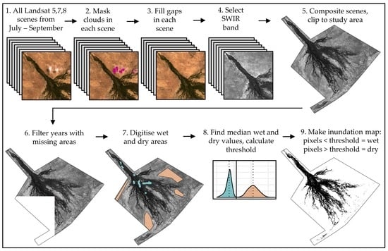
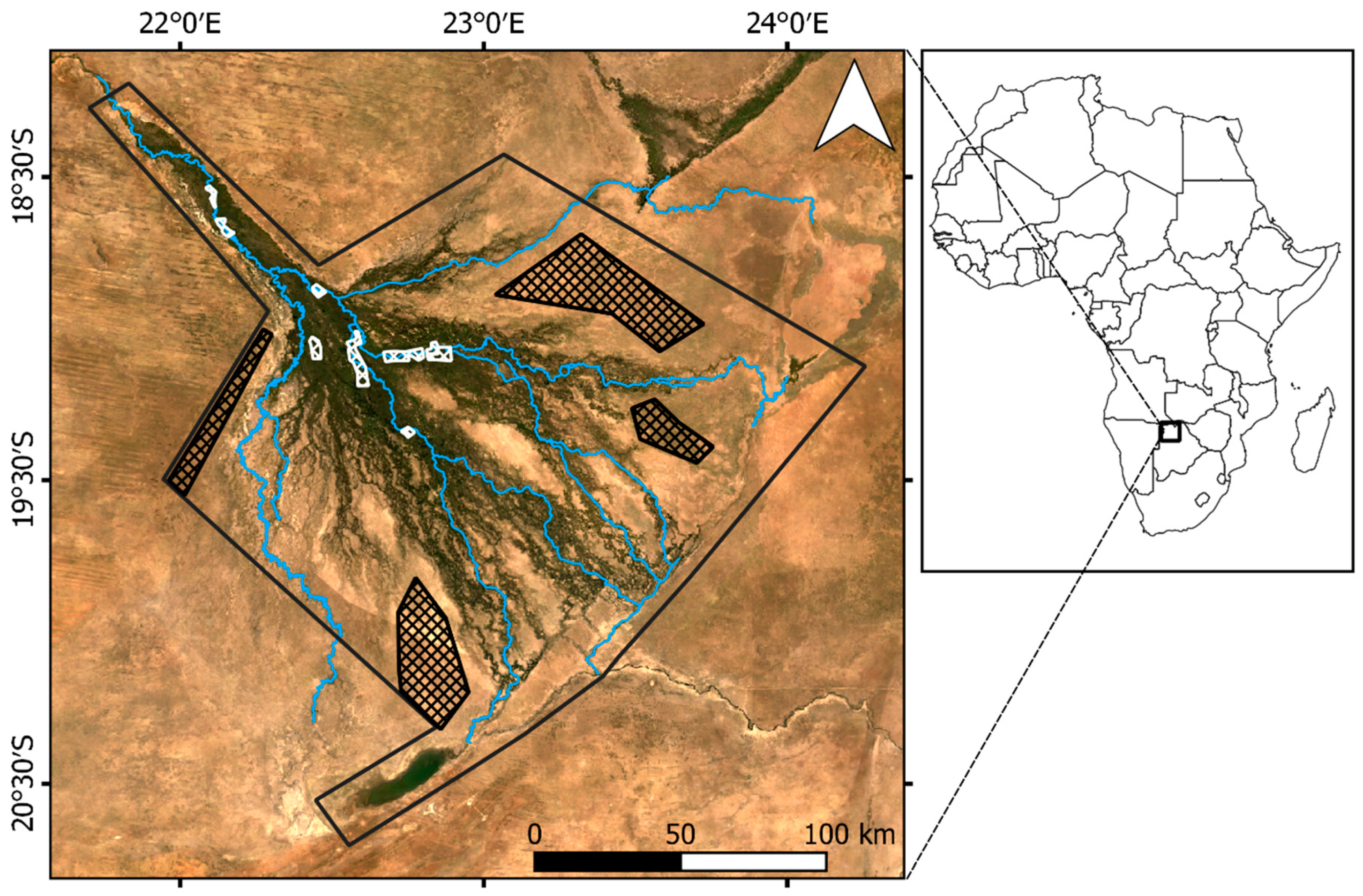
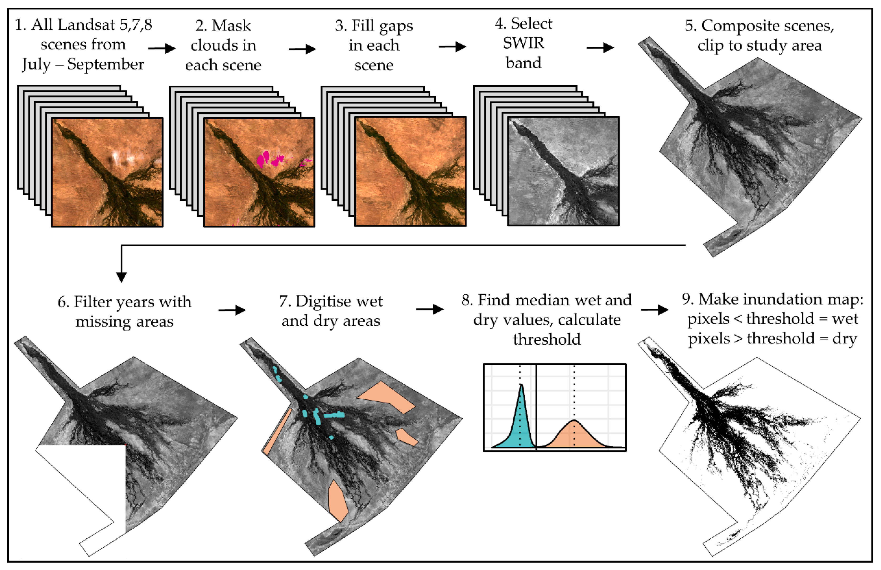
2.1. Annual (July–September) Landsat Composites

Unless otherwise stated, all processing was conducted using Google Earth Engine. Every tier 1 atmospherically corrected surface reflectance Landsat (Landsat 5 TM, Landsat 7 ETM+, Landsat 8 OLI) scene covering the Okavango Delta (Figure 1) for the peak inundation period (1 July to 30 September) from 1990 to 2019 was used (Step 1 in Figure 2). Scenes occurred within six Landsat path/row footprints (174/073, 174/074, 175/073, 175/074, 176/072, 176/073). These sensors capture scenes with 30 m spatial resolution, containing eight (Landsat 5 and 7) and eleven (Landsat 8) bands, including the SWIR band (band 7) used in this study. For each scene, pixels classified as cloud or cloud shadow on the Landsat cloud mask band were masked (Step 2 in Figure 2). These pixels were then filled using the median value for the pixel from a year before and after the scenes’ date, using a gap-filling algorithm [34] (step 3 in Figure 2). The SWIR band was selected for each scene (step 4 in Figure 2) and then, for each year, a composite was created from the median value of all the scenes for that year (step 5 in Figure 2). Annual composites with large areas missing (e.g., there were no scenes available for a path/row) were filtered out (step 6 in Figure 2). This occurred five times (1993, 2000, 2009, 2010, and 2012).

2.2. Annual (July–September) Inundation Maps

The composites were transformed into inundation maps using an SWIR thresholding technique. To apply this method, we assessed and digitised areas that had permanent water (e.g., permanent swamp or main channels) or were permanently dry, based on Wolski et al.’s [9] designated areas, but altered slightly to suit our use of higher spatial resolution imagery (Figure 1, step 7 in Figure 2). The median SWIR value for the inundated (SWIRwet) and dry (SWIRdry) areas was calculated for each individual composite, and a composite-specific SWIRthreshold value was calculated using Equation (1) (taken from Wolski et al. [9]) (step 8 in Figure 2).
SWIRthreshold = SWIRwet + 0.3 ∗(SWIRdry − SWIRwet)
The relative frequency of SWIR values for the wet and dry areas is shown in Figure S1, with the SWIRwet, SWIRdry, and SWIRthreshold values marked. Pixels with an SWIR value below the threshold were classified as inundated, and vice-versa for dry pixels (step 9 in Figure 2). Calculating the threshold value separately for each image accounts for the dynamic (seasonal and annual) nature of the inundation patterns of the delta [9]. The multiplier of 0.3 represents the value needed to calculate the correct threshold to classify a pixel with an inundation fraction of 50% as inundated, as recommended by Wolski et al. [9]. Owing to the different imagery used in this study, we confirmed the value of 0.3 was appropriate, by also assessing inundation maps developed using values of 0.25 and 0.35 (see next section). Further details about this classification method and its development are provided in Wolski et al. [9].

2.3. Validating Inundation Maps (Image-Based Accuracy Assessment)

Gathering in situ data for historical time series is difficult, and in many cases, these data simply do not exist. To enable validation for at least some of the time series, we used a visual interpretation approach to generate reference data. Although this method can be subjective, it is a generally accepted approach, particularly when historical data are limited [2,35,36,37,38,39,40,41]. We validated the accuracy of three sets of inundation maps (produced using 0.25, 0.3, and 0.35 in Equation (1)) by visual assessment of true colour versions of the Landsat composites used to make the inundation maps, and high-resolution satellite images. The inundation maps were created without filling masked pixels, and only comprised a subset of the years (2000–2016). High resolution imagery taken between July and October was accessed via Google Earth’s historical imagery function and the Digital Globe collection (obtained from the DigitalGlobe Foundation). Given that the study area (Figure 1) included large tracts of permanently dry areas (i.e., the Kalahari Desert), which we predicted would rarely be misclassified [9], we used an amended area for the validation, removing some of the larger dry areas (Figure S2). Using this amended area, fifty sample points (Figure S2) were randomly generated using the sampleRandom function (raster package [42]) in R [43]. For each year, the same 50 sample points were visually assigned as inundated or dry on the Landsat and high-resolution imagery before progressing onto the next year. This prevented the assessors from making classifications based on a sample point’s previous inundation history. The classification (inundated or dry) of each sample point was extracted from the relevant inundation map and an error matrix was created. Overall accuracy (the sum of the diagonal entries (correctly classified points) divided by the total sampled points), producer’s accuracy (the diagonal entry divided by its respective column total), and user’s accuracy (the diagonal entry of each row divided by its respective row total) were calculated.

2.4. Validating Inundation Maps (In Situ Data Accuracy Assessment)

To validate the accuracy of the classification method, we carried out a field examination of inundated and dry regions within one Landsat scene (scene 175/73, 25 July 2018). Owing to accessibility and safety constraints, we only sampled from the Abu Concession (Figure S3), where inundated areas could be accessed by field personnel by wading (within 100 m of dry land). Sampling points were chosen using a random stratified sampling approach, where inundated and dry were the stratification levels. The sampling area was created in QGIS [44] by outlining islands that were accessible by vehicle, applying a 100 m buffer, and clipping the inundation map to this shape. The raster was imported into R [43] and 55 points in each stratum were randomly selected (Figure S3) using the sampleStratified function (raster package [42]), which were then exported and uploaded to a handheld Garmin GPSMAP® 64 GPS. This number of sample points was chosen to ensure that if some points were inaccessible (e.g., vegetation too thick to drive through, unsafe to wade into water, wildlife within close proximity), the recommended minimum number of 50 [35] could still be obtained. Data collection occurred within two days of the sensor’s collection of the scene (25–27 July 2018), with each point classified as either inundated (standing water) or dry, based on which class occurred over the majority of the 30 m2 area centered on each point. Where the proportion of each class was approaching equality, the point was classified, but was also noted as an uncertain classification. The classification for each sample point was extracted from the inundation map created from the Landsat scene and an error matrix was created. Overall accuracy, user’s accuracy, and producer’s accuracy were calculated as above.

3. Results

The extent and distribution of the peak inundation varied annually (Figure 3 and Figure 4), with the smallest inundation extent occurring in 2019 (3487 km2) and the greatest in 2011 (10,109 km2) (Figure 4 and Figure 5). The average inundation extent was 6635 km2. The SWIRthreshold values ranged from 1306 (2014) to 1637 (2003) (Figure S1), emphasising the importance of calculating this variable individually for each composite. On average, estimates of inundation extent were 692 km2 smaller than those from previous studies, which used MODIS (250 m and 500 m spatial resolution) and NOAA AVHRR (1000 m spatial resolution) imagery, with a maximum difference of 2373 km2 (Figure 4).

Validating Inundation Maps

Using the true colour Landsat composites, a total of 691 points were visually classified; fifty points per year, except for years without inundation maps and 2010 and 2011, where five and four validation pixels were masked, respectively. There were fewer points (123) visually classified using the high-resolution imagery owing to a lack of available data. For inundation maps created using a multiplier of 0.3, based on the visual assessment of Landsat composites, the inundation maps had few misclassified pixels (1.9%), but this was slightly higher based on the visual classification of high-resolution imagery (4.1%) (Table 1). Inundation maps created using a value of 0.25 had slightly lower overall accuracy, and using a value of 0.35 had almost identical overall accuracy (Table S1). Misclassified points were located predominately on the boundary of inundated and dry areas and where there was high inter-annual variation in inundation (Figure S2).
Out of the 110 sample points that were generated for the in situ validation, we classified 106 (four were inaccessible). The inundation map had an overall accuracy of 91.5% (nine sample points were misclassified) (Table 1, Figure S3). Of these nine misclassified points, seven were noted as uncertain in the field as they had approximately equal areas of inundation and dry. There was an additional uncertain point that was correctly classified. When these uncertain points were removed, overall accuracy increased to 98.0% (Table 1).

4. Discussion

Our study details the longest ever time series of peak flooding extents for the Okavango Delta at a high spatial resolution (30 m), demonstrating the remarkable inter-annual variability of this system; the largest inundation extent recorded was almost three times that of the smallest (Figure 4 and Figure 5). There are also inter-annual variations in the spatial distribution of inundation (Figure 3 and Figure 5, Data S1 (annual rasters)), driven by the volume of water discharged into the system, but also factors such as sedimentation, channel blockage from vegetation, and avulsion [6,8,45,46]. On the basis of the maps produced in this study, the 2019 flood event represents the smallest inundation since 1985, being around 769 km2 smaller than the previous record in 1996 (Figure 4). Estimations of inundation extent going back to 1934 calculated the lowest inundation to be approximately 5100 km2 [6]. Our estimate of inundation extent in 2019 was 3483 km2, making it the smallest flood in the last 85 years. This exceptionally low flood is likely driven by a multi-decadal (16–20 years) rainfall cycle in Southern Africa [6,47,48], being 14 years since the previous dry year. The delta is also at risk of drying owing to increases in temperature and evaporation and decreases in rainfall and river flow due to climate change and water abstraction and damming [4,49].
The annual inundation extent estimates in our study were systematically smaller than previous studies, but showed a similar trend (Figure 4). The most likely cause for this effect is our use of higher resolution imagery, an effect that is also evident in other study systems when comparing estimates from different sensor resolutions [50,51,52,53]. Broad spatial resolution imagery (as used in existing studies) increases the number of mixed pixels, and can lead to overestimations of the size of the inundated areas [4,29], which we reduced by using Landsat images. Another potential cause for smaller estimates is our use of three-month composites rather than individual consecutive images, concealing the time of true maximum inundation, although our use of median values should be robust to this effect.
Accuracy assessments of delta inundation maps have generally not included in situ data (Murray-Hudson et al. [15] is an exception), instead using comparisons to high resolution aerial orthomosaics [2], other inundation maps [8,9,15], or hydrological observations [6,9]. The overall accuracy of the method used in this study as determined by the image-based assessment (95.9%–98.1%) is comparable to these other studies, being predictably higher for the Landsat composites than the independent high-resolution images, as these are the true colour version of the images on which the inundation maps were based. Also contributing to the reduced accuracy, high-resolution images covered a slightly longer time period (July–October) than that used to make the inundation maps (done to increase available data), and were individual images, as opposed to composites, meaning they may have occurred before/after the full extent of the flood. Although only a subset of the maps (2000–2016) was validated, Figure S1 provides further evidence that the thresholding method can accurately detect the boundary between inundated and dry pixels, with non-validated and validated years following a similar pattern.
The overall accuracy from in situ data validation (91.5%) was slightly lower than from the image-based assessment, although not so (98.0%) when we removed points we had flagged as uncertain in the field. These were points that were approximately half inundated and half dry (i.e., a mixed pixel) and had remaining moisture in the soil (i.e., were muddy) where the flood had recently receded (but which we classified as dry as there was no standing water) (Figure S3). In situ data collection in this area is difficult owing to logistics, accessibility, and safety issues, particularly during the high flood period [2,4,10,54]; so, while our in situ validation was small in scale, it represents a rarely conducted true accuracy assessment of delta inundation mapping. In addition, given that the sampling area was centered on small islands and edges of the floodplain, it fittingly represents the boundary between dry and inundated areas, the area where most classification errors are likely to occur [9] (Figure S2), and which was under-represented in the sample points of the image-based accuracy assessment. Therefore, the high accuracy within this sampling area suggests the overall delta wide classification is likely to be reliable, confirmed by the delta-wide image-based validation.
In addition to inaccuracy caused by mixed pixels, we noted, as did Wolski et al. [9], the presence of some true misclassification when using this method. Visual inspection of our maps suggests riparian woodland vegetation is sometimes misclassified as inundated area, a known problem in the delta where these classes can have overlapping spectral signatures [2] and where riparian woodland can saturate Landsat pixels [14]. A potential solution to minimise this would be filtering out pixels that are discontinuous from the larger inundated area [2], although for the sake of simplicity, we have not attempted to do this. Misclassifications can also occur where there is a small difference between the SWIR value of the dry and inundated areas used for the threshold calculation, typically during the wet season [9], which this study did not measure. The anomalously low flood level in 2019 meant it was difficult to get suitable training data that were consistent with the other maps. Therefore, dry pixels within the permanent water polygon increased the range of SWIRwet values (Figure S1). This may have led to a higher level of misclassification (Figure 5).
Choosing a sensor is a compromise between spatial and temporal resolution and the computational time and power required to process the images. Google Earth Engine allowed us to take advantage of high-resolution images with minimal effort; all images are called directly to the software without downloading and functions (e.g., cloud masking) can be automated. In an ecosystem as complex as the delta, broad spatial resolution maps may have restricted utility [6]. Using 500 m spatial resolution imagery, Wolski et al. [9] noted that some important terminal rivers of the delta were not well represented on their inundation maps as they were narrower than the resolution of the imagery. However, by using Landsat imagery, the mosaic of floodplains and islands are well represented, and rivers that are important indicators of the hydrology of the delta, as well as essential to local communities (e.g., the Thamalakane River), are clearly mapped (Figure 3).

5. Conclusions

Wolski et al. [9] developed a simple method (thresholding of the short wave infrared band) to accurately classify inundation in the Okavango Delta using broad spatial resolution (500 m) satellite imagery, noting the method was suitable for automation, but also cautioning that creating inundation maps using Landsat imagery was “laborious … making creation of a consistent, long time series of inundation maps difficult”. In this paper, we have shown that periodic, accurate inundation maps can be created using relatively high-resolution imagery (Landsat) suitable to capture the complexity of this important ecosystem, by utilizing Google Earth Engine, a cloud-based platform. We provide the longest time series (1990–2019) of inundation maps for the peak flood season at a relatively high spatial resolution (30 m) to date. The inaccessibly of remote sensing methods and processing capability has prevented wide-spread adoption of its use by non-experts. We anticipate that the methods/code and the data produced in this paper can be used and adapted by land managers, researchers, and other stakeholders, who require access to accurate high resolution inundation maps. Further, the classification method is likely to be suitable for mapping inundation in other regions, with only minimal adaptation of the methods and code presented here.

Supplementary Materials

The following are available online at https://www.mdpi.com/2072-4292/12/8/1348/s1, Figure S1: Density of SWIR values for permanent water and dry areas, with median values (dashed line) and threshold value (solid line) for each year; Figure S2: Location of validation points for image-based accuracy assessment. Black points were always correctly classified, red points were incorrectly classified at least once (label displays the number of times incorrectly classified out of total times classified). Dashed line represents amended area for point sampling and background map is the summed annual inundation map; Figure S3: In situ accuracy assessment of a single inundation map (25 July 2018) showing (a) all sampling points and their classifications and examples of (b) an incorrectly classified point that was classed as uncertain in the field, (c) a correctly classified inundated point, and (d) a correctly classified dry point. Overview map shows average inundation extent; Table S1: Error matrices and overall accuracy of inundation maps using image-based accuracy assessment (Landsat and high-resolution imagery) using alternative values of f in the threshold equation SWIRthreshold = SWIRwet + f ∗(SWIRdry − SWIRwet); Data S1: Rasters of individual inundation maps (1990–2019); Data S2: Raster of sum of all inundation maps; Data S3: Raster of variance of all inundation maps; Data S4: Annual inundation extents; Code S1: Google Earth Engine code and inundation rasters are available on Github (https://github.com/VictoriaInman/OkavangoDelta_flooding) and archived on Zenodo (DOI: 10.5281/zenodo.3693153); Code S2: Link to Google Earth Engine repository https://code.earthengine.google.com/?accept_repo=users/victoriainman/OkavangoDelta_TechnicalNote.

Author Contributions

V.L.I. led the conceptualization, data collection, analysis, and writing; M.B.L. contributed to analysis and writing. All authors have read and agreed to the published version of the manuscript.

Funding

This research received no external funding.

Acknowledgments

We thank Elephants without Borders for hosting V.L.I.’s fieldwork where in situ data were collected, and to Keboditse “CK” Mboroma for his assistance in the field. In addition, we thank the Botswana Ministry of Environment, Wildlife, and Tourism for affording us the opportunity to conduct the fieldwork. Thanks to John Wilshire for helping with Google Earth Engine and to Piotr Wolski for his advice on adapting his method to Landsat imagery and providing shapefiles for the permanently inundated and dry areas.

Conflicts of Interest

The authors declare no conflict of interest. The funders had no role in the design of the study; in the collection, analyses, or interpretation of data; in the writing of the manuscript; or in the decision to publish the results.

References

  1. Milzow, C.; Kgotlhang, L.; Bauer-Gottwein, P.; Meier, P.; Kinzelbach, W. Regional review: The hydrology of the Okavango Delta, Botswana—Processes, data and modelling. Hydrogeol. J. 2009, 17, 1297–1328. [Google Scholar] [CrossRef]
  2. Wolski, P.; Murray-Hudson, M. Reconstruction 1989-2005 inundation history in the Okavango Delta from archival LandSat TM imagery. In Proceedings of the Globewetlands Symposium, ESA-ESRIN, Rome, Italy, 19–20 October 2006. [Google Scholar]
  3. Ramsar Ramsar Sites Information Service. Available online: https://rsis.ramsar.org/ (accessed on 18 November 2019).
  4. Milzow, C.; Kgotlhang, L.; Kinzelbach, W.; Meier, P.; Bauer-Gottwein, P. The role of remote sensing in hydrological modelling of the Okavango Delta, Botswana. J. Environ. Manag. 2009, 90, 2252–2260. [Google Scholar] [CrossRef]
  5. Gumbricht, T.; McCarthy, J.; McCarthy, T.S. Channels, wetlands and islands in the Okavango Delta, Botswana, and their relation to hydrological and sedimentological processes. Earth Surf. Process. Landf. 2004, 29, 15–29. [Google Scholar] [CrossRef]
  6. Gumbricht, T.; Wolski, P.; Frost, P.; McCarthy, T.S. Forecasting the spatial extent of the annual flood in the Okavango Delta, Botswana. J. Hydrol. 2004, 290, 178–191. [Google Scholar] [CrossRef]
  7. McCarthy, T.S.; Bloem, A.; Larkin, P.A. Observations on the hydrology and geohydrology of the Okavango Delta. S. Afr. J. Geol. 1998, 101, 101–117. [Google Scholar]
  8. Thito, K.; Wolski, P.; Murray-Hudson, M. Mapping inundation extent, frequency and duration in the Okavango Delta from 2001 to 2012. Afr. J. Aquat. Sci. 2016, 41, 267–277. [Google Scholar] [CrossRef]
  9. Wolski, P.; Murray-Hudson, M.; Thito, K.; Cassidy, L. Keeping it simple: Monitoring flood extent in large data-poor wetlands using MODIS SWIR data. Int. J. Appl. Earth Obs. Geoinf. 2017, 57, 224–234. [Google Scholar] [CrossRef] [Green Version]
  10. McCarthy, J.M.; Gumbricht, T.; McCarthy, T.; Frost, P.; Wessels, K.; Seidel, F. Flooding patterns of the Okavango Wetland in Botswana between 1972 and 2000. Ambio 2003, 32, 453–457. [Google Scholar] [CrossRef]
  11. Department of Environmental Affairs. Okavango Delta Management Plan; Ministry of Environment, Wildlife, and Tourism: Gaborone, Botswana, 2008.
  12. Ramberg, L.; Hancock, P.; Lindholm, M.; Meyer, T.; Ringrose, S.; Sliva, J.; Van As, J.; VanderPost, C. Species diversity of the Okavango Delta, Botswana. Aquat. Sci. 2006, 68, 310–337. [Google Scholar] [CrossRef]
  13. Fluet-Chouinard, E.; Lehner, B.; Rebelo, L.M.; Papa, F.; Hamilton, S.K. Development of a global inundation map at high spatial resolution from topographic downscaling of coarse-scale remote sensing data. Remote Sens. Environ. 2015, 158, 348–361. [Google Scholar] [CrossRef]
  14. Ringrose, S.; Vanderpost, C.; Matheson, W. Mapping ecological conditions in the Okavango delta, Botswana using fine and coarse resolution systems including simulated SPOT vegetation imagery. Int. J. Remote Sens. 2003, 24, 1029–1052. [Google Scholar] [CrossRef]
  15. Murray-Hudson, M.; Wolski, P.; Cassidy, L.; Brown, M.T.; Thito, K.; Kashe, K.; Mosimanyana, E. Remote Sensing-derived hydroperiod as a predictor of floodplain vegetation composition. Wetl. Ecol. Manag. 2015, 23, 603–616. [Google Scholar] [CrossRef]
  16. Islam, A.S.; Bala, S.K.; Haque, M.A. Flood inundation map of Bangladesh using MODIS time-series images. J. Flood Risk Manag. 2010, 3, 210–222. [Google Scholar] [CrossRef]
  17. Kalluri, S.; Gilruth, P.; Bergman, R. The potential of remote sensing data for decision makers at the state, local and tribal level: Experiences from NASA’s Synergy program. Environ. Sci. Policy 2003, 6, 487–500. [Google Scholar] [CrossRef]
  18. Ouellette, W.; Getinet, W. Remote sensing for Marine Spatial Planning and Integrated Coastal Areas Management: Achievements, challenges, opportunities and future prospects. Remote Sens. Appl. Soc. Environ. 2016, 4, 138–157. [Google Scholar] [CrossRef]
  19. Hermon, D. Land Stability Model for Sustainable Spatial Planning in Padang City-Indonesia based on Landslide Disaster. J. Geogr. Earth Sci. 2019, 7, 19–26. [Google Scholar] [CrossRef]
  20. Heiskanen, J.; Liu, J.; Valbuena, R.; Aynekulu, E.; Packalen, P.; Pellikka, P. Remote sensing approach for spatial planning of land management interventions in West African savannas. J. Arid Environ. 2017, 140, 29–41. [Google Scholar] [CrossRef] [Green Version]
  21. Seto, K.C.K.; Woodcock, C.E.C.E.; Song, C.; Huang, X.; Lu, J.; Kaufmann, R.K. Monitoring land-use change in the Pearl River Delta using Landsat TM. Int. J. Remote Sens. 2002, 23, 1985–2004. [Google Scholar] [CrossRef]
  22. Fu, P.; Weng, Q. A time series analysis of urbanization induced land use and land cover change and its impact on land surface temperature with Landsat imagery. Remote Sens. Environ. 2016, 175, 205–214. [Google Scholar] [CrossRef]
  23. Allen, R.G.; Tasumi, M.; Morse, A.; Trezza, R. A landsat-based energy balance and evapotranspiration model in Western US water rights regulation and planning. Irrig. Drain. Syst. 2005, 19, 251–268. [Google Scholar] [CrossRef]
  24. Bechtel, R.; Sánchez-Azofeifa, A.; Rivard, B.; Hamilton, G.; Martin, J.; Dzus, E. Associations between Woodland Caribou telemetry data and Landsat TM spectral reflectance. Int. J. Remote Sens. 2004, 25, 4813–4828. [Google Scholar] [CrossRef]
  25. Simons-Legaard, E.M.; Harrison, D.J.; Legaard, K.R. Habitat monitoring and projections for Canada lynx: Linking the Landsat archive with carnivore occurrence and prey density. J. Appl. Ecol. 2016, 53, 1260–1269. [Google Scholar] [CrossRef] [Green Version]
  26. Ticehurst, C.; Dutta, D.; Karim, F. Improving the accuracy of daily MODIS OWL flood inundation mapping using hydrodynamic modelling. Nat. Hazards 2015, 78, 803–820. [Google Scholar] [CrossRef]
  27. Chen, Y.; Huang, C.; Ticehurst, C.; Merrin, L.; Thew, P. An Evaluation of MODIS Daily and 8-day Composite Products for Floodplain and Wetland Inundation Mapping. Wetlands 2013, 33, 823–835. [Google Scholar] [CrossRef]
  28. Fayne, J.V.; Bolten, J.D.; Doyle, C.S.; Fuhrmann, S.; Matthew, T.; Houser, P.R.; Lakshmi, V.; Fayne, J.V.; Bolten, J.D.; Doyle, C.S.; et al. Flood mapping in the lower Mekong River Basin using daily MODIS observations Flood mapping in the lower Mekong River Basin using daily MODIS observations. Int. J. Remote Sens. 2017, 38, 1737–1757. [Google Scholar] [CrossRef]
  29. Danaher, T.; Flood, N. A Comparison of Woody Change Mapping based on SPOT 5 and Landsat TM Imagery Using 2010—2011 Imagery; Office of Environment and Heritage: Sydney, Australia, 2014.
  30. Li, L.; Chen, Y.; Yu, X.; Liu, R.; Huang, C. Sub-pixel flood inundation mapping from multispectral remotely sensed images based on discrete particle swarm optimization. ISPRS J. Photogramm. Remote Sens. 2015, 101, 10–21. [Google Scholar] [CrossRef]
  31. Verhoeye, J.; De Wulf, R. Land cover mapping at sub-pixel scales using linear optimization techniques. Remote Sens. Environ. 2002, 79, 96–104. [Google Scholar] [CrossRef]
  32. Gorelick, N.; Hancher, M.; Dixon, M.; Ilyushchenko, S.; Thau, D.; Moore, R. Google Earth Engine: Planetary-scale geospatial analysis for everyone. Remote. Sens. Environ. 2017, 202, 18–27. [Google Scholar] [CrossRef]
  33. Thalefang, C. Why Okavango Delta is drying—Experts speak. Mmegi Online. 2019, pp. 1–11. Available online: https://www.mmegi.bw/index.php?aid=82034&dir=2019%2Faugust%2F02 (accessed on 2 March 2020).
  34. Scaramuzza, P.; Micijevic, E.; Chander, G. SLC-Off Gap-Filled Products: Gap-Fill Algorithm Methodology; US Geological Survey Earth Resources Observation and Science (EROS) Center, 2004. Available online: https://landsat.usgs.gov/sites/default/files/documents/L7SLCGapFilledMethod.pdf (accessed on 2 March 2020).
  35. Olofsson, P.; Foody, G.M.; Herold, M.; Stehman, S.V.; Woodcock, C.E.; Wulder, M.A. Good practices for estimating area and assessing accuracy of land change. Remote Sens. Environ. 2014, 148, 42–57. [Google Scholar] [CrossRef]
  36. Iwao, K.; Nishida, K.; Kinoshita, T.; Yamagata, Y. Validating land cover maps with Degree Confluence Project information. Geophys. Res. Lett. 2006, 33, 1–5. [Google Scholar] [CrossRef]
  37. Montesano, P.M.; Nelson, R.; Sun, G.; Margolis, H.; Kerber, A.; Ranson, K.J. MODIS tree cover validation for the circumpolar taiga – tundra transition zone. Remote Sens. Environ. 2009, 113, 2130–2141. [Google Scholar] [CrossRef] [Green Version]
  38. Luedeling, E.; Buerkert, A. Typology of oases in northern Oman based on Landsat and SRTM imagery and geological survey data. Remote Sens. Environ. 2008, 112, 1181–1195. [Google Scholar] [CrossRef]
  39. Bastin, L.; Buchanan, G.; Beresford, A.; Pekel, J.; Dubois, G. Ecological Informatics Open-source mapping and services for Web-based land-cover validation. Ecol. Inform. 2013, 14, 9–16. [Google Scholar] [CrossRef] [Green Version]
  40. Strand, G.; Dramstad, W.; Engan, G. The effect of field experience on the accuracy of identifying land cover types in aerial photographs. Int. J. Appl. Earth Obs. Geoinf. 2002, 4, 137–146. [Google Scholar] [CrossRef]
  41. Silvestri, S.; Omri, M. A method for the remote sensing identification of uncontrolled landfills: Formulation and validation. Int. J. Remote Sens. 2008, 29, 975–989. [Google Scholar] [CrossRef]
  42. Hijmans, R.J. raster: Geographic Data Analysis and Modeling. R Package Version 3.0-7. 2019. Available online: http://CRAN.R-project.org/package=raster (accessed on 2 March 2020).
  43. R Core Team. R: A Language and Environment for Statistical Computing; R Foundation for Statistical Computing: Vienna, Austria, 2018. [Google Scholar]
  44. QGIS Development Team. QGIS Geographic Information System. Open Source Geospatial Foundation Project. 2018. Available online: http://qgis.osgeo.org (accessed on 2 March 2020).
  45. Wolski, P.; Murray-Hudson, M. Recent changes in flooding in the Xudum distributary of the Okavango Delta and Lake Ngami, Botswana. S. Afr. J. Sci. 2006, 102, 173–176. [Google Scholar]
  46. McCarthy, T.S.; Ellery, W.N.; Stanistreet, I.G. Avulsion mechanisms on the Okavango fan, Botswana: The control of a fluvial system by vegetation. Sedimentology 1992, 39, 779–795. [Google Scholar] [CrossRef]
  47. McCarthy, T.S.; Cooper, G.R.J.; Tyson, P.D.; Ellery, W.N. Seasonal flooding in the Okavango Delta, Botswana—Recent history and future prospects. S. Afr. J. Sci. 2000, 96, 25–33. [Google Scholar]
  48. Tyson, P.D.; Cooper, G.R.J.; McCarthy, T.S. Millennial to multi-decadal variability in the climate of southern Africa. Int. J. Climatol. 2002, 22, 1105–1117. [Google Scholar] [CrossRef]
  49. Murray-Hudson, M.; Wolski, P.; Ringrose, S. Scenarios of the impact of local and upstream changes in climate and water use on hydro-ecology in the Okavango Delta, Botswana. J. Hydrol. 2006, 331, 73–84. [Google Scholar] [CrossRef]
  50. Hlavka, C.A.; Livingston, G.P. Statistical models of fragmented land cover and the effect of coarse spatial resolution on the estimation of area with satellite sensor imagery. Int. J. Remote Sens. 1997, 18, 2253–2259. [Google Scholar] [CrossRef]
  51. Loboda, T. Estimating burned area from AVHRR and MODIS: Validation results and sources of error. Proc. Curr. Asp. Rem. 2004, 2, 415–421. [Google Scholar]
  52. Moody, A.; Woodcock, C.E. Scale-dependent errors in the estimation of land-cover proportions: Implications for global land-cover datasets. Photogramm. Eng. Remote Sens. 1994, 60, 585–594. [Google Scholar]
  53. Ozdogan, M.; Woodcock, C.E. Resolution dependent errors in remote sensing of cultivated areas. Remote Sens. Environ. 2006, 103, 203–217. [Google Scholar] [CrossRef]
  54. McCarthy, J. Remote Sensing for Detection of Landscape Form and Function of the Okavango Delta Botswana. Ph.D. Thesis, Department of Land and Water Resources Engineering, KTH, Stockholm, Sweden, 12 April 2002. ISBN 9172832495. Available online: kth.diva-portal.org/smash/record/jsf?pid=diva2%3A9101&dswid=4172 (accessed on 2 March 2020).
Figure 1. Okavango Delta study area (black outline) in northern Botswana. White and black hatched areas are the permanent water (permanent swamps and channels) and dry areas, respectively, used in calculating the threshold value, and blue lines are the major channels of the delta.
Remotesensing 12 01348 g001
Figure 2. Schematic displaying the process of creating an annual inundation map. Steps are detailed in text. SWIR, short wave infrared.
Remotesensing 12 01348 g002
Figure 3. Summed annual inundation map for the time series (30-year span, 25 individual flood maps) showing the inter-annual variation in peak flood extent.
Remotesensing 12 01348 g003
Figure 4. Annual (July–September) inundation extent (km2) of the Okavango Delta from our data and other studies. Inundation maps from other studies were developed using imagery predominately from MCD43A4 (500m spatial resolution) (Wolski et al. 2017 [9]), MOD09Q (250 m spatial resolution) (Thito et al. 2016 [8]), and NOAA AVHRR (1000 m) (Gumbricht et al. 2004, McCarthy et al. 2003 [6,10]). Note: inundation extents from other studies were taken from tables and figures (using http://www.graphreader.com/) for the same months as those used in this study.
Remotesensing 12 01348 g004
Figure 5. ‘Natural’ colour composite (short wave infrared (SWIR), near infrared (NIR), green bands), SWIR band composite, and inundation map (black area is inundated) for years with minimum, mean, and maximum flood extent. In 2019, inundated pixels in the southwest of the map are likely misclassified. Note: flood extent in 2005 was within 100 km2 of average flood extent.
Remotesensing 12 01348 g005
Table 1. Error matrices and overall accuracy of inundation maps using image-based accuracy assessment (Landsat and high-resolution imagery) and in situ points. Note: values in square brackets are based on points noted as ‘uncertain’ being removed.
LandsatHi-res Visual Interp.In Situ
DryWetDryWetDryWet
MapDry5261082345 [44]1 [0]
Wet31522368 [2]52 [52]
Overall accuracy98.1% (678/691)95.9% (118/123)91.5% (97/106)
[98.0% (96/98)]
Producer’s accuracy—Landsat, dry = 99.4% (526/529) and wet = 93.8% (152/162); high-resolution imagery, dry = 97.6% (82/84) and wet = 92.3% (36/39); in situ, dry = 84.9% (45/53) [95.7% (44/46)] and wet = 98.1% (52/53) [100% (52/52)]. User’s accuracy—Landsat, dry = 98.1% (526/536) and wet = 98.1% (152/155); high-resolution imagery, dry = 96.5% (82/85) and wet = 94.7% (36/38); in situ, dry = 97.8% (45/46) [100% (44/44)] and wet = 86.7% (52/60) [96.3% (52/54)].

