
An Assessment of CyGNSS v3.0 Level 1 Observables over the Ocean


National Oceanography Centre, Southampton SO14 3ZH, UK
*
Author to whom correspondence should be addressed.
Remote Sens. 2021, 13(17), 3500; https://doi.org/10.3390/rs13173500
Submission received: 9 July 2021
/
Revised: 15 August 2021
/
Accepted: 21 August 2021
/
Published: 3 September 2021
(This article belongs to the Special Issue Remote Sensing of Ocean Surface Winds)
Abstract
:Global Navigation Satellite System Reflectometry (GNSS-R) is a rapidly developing Earth observation technology that makes use of signals of opportunity from Global Navigation Satellite Systems that have been reflected off the Earth’s surface. The Cyclone Global Navigation Satellite System (CyGNSS) is a constellation of eight small satellites launched by NASA in 2016, carrying dedicated GNSS-R payloads to measure ocean surface wind speed at low latitudes (±35° North/South). The ESA ECOLOGY project evaluated CyGNSS v3.0 products, which were recently released following various calibration updates. This paper examines the performance of the new calibration by evaluating CyGNSS v3.0 Level-1 Normalised Bistatic Radar Cross Section (NBRCS) and Leading Edge Slope (LES) data from individual CyGNSS units and different GPS transmitters under constant ocean wind conditions. Results indicate that L1 NBRCS from individual CyGNSS units are well inter-calibrated and remarkably stable over time, a significant improvement over previous versions of the products. However, prominent geographical biases reaching over 3 dB are found in NBRCS, linked to factors including the choice of GPS transmitter and the bistatic geometry. L1 LES shows similar anomalies as well as a secondary geographical pattern of biases. These findings provide a basis for further improvement of CyGNSS Level-2 wind products and have wider applicability to improving the calibration of GNSS-R sensors for the remote sensing of non-ocean Earth surfaces.
1. Introduction
Following the first proposal of the GNSS-R principle for scatterometry in the late 1980s [1], and later in the early 1990s for ocean altimetry [2], the technology was later demonstrated from low-Earth-orbit altitudes by the UK-Disaster Monitoring Constellation (UK-DMC) [3] and UK TechDemoSat-1 (TDS-1) missions [4,5]. It has since been implemented as a dedicated mission with the NASA CyGNSS constellation of small satellites [6]. GNSS-R receivers detect and correlate reflected GNSS signals with the direct signals from the same GNSS transmitter to produce delay Doppler maps (DDMs). GNSS-R is particularly promising as it does not require a dedicated transmitter, thereby reducing the cost, mass, and power requirements of the instrument. These advantages offer the potential to deploy GNSS-R sensors as payloads of opportunity aboard other missions or as low-cost multi-satellite constellations.
Examining the correlation between the reflected and direct signals allows inference of a number of Earth surface parameters, which can be broadly categorised as being associated with surface reflectivity (scatterometry) or surface elevation (altimetry). GNSS-R has been particularly well demonstrated for the remote sensing of ocean wind speed [5,7,8,9], and also for other geophysical variables including sea ice and soil moisture [10,11]. Retrieval of ocean wind speed works on the principle of increased wind speed driving an increase in the mean square slope (MSS) of waves. The normalised bistatic radar cross-section (NBRCS) describes the strength of the signal scattered of the rough surface in the direction of the receiver’s antenna, which will decrease with an increase in MSS, as detailed by the bistatic radar equation [12].
NASA CyGNSS is a constellation of eight small satellites (aka flight models, or FM) with GNSS-R receivers as the unique scientific payload. CyGNSS has the primary objective of measuring wind speed in hurricanes and tropical cyclones with high temporal frequency [13]. This goal is addressed by using a constellation of eight satellites in a low inclination orbital plane to enable rapid revisit times (of the order of hours). In addition, the use of L-band microwave signals (GPS L1 wavelength ~19 cm) should make GNSS-R less sensitive to attenuation due to the presence of water vapour or liquid rain in the atmosphere, as in the case of tropical cyclones. Since launch, CyGNSS GNSS reflections have also been shown to be sensitive to other geophysical parameters, including soil moisture content, aboveground biomass, and inundation [11,14], providing an opportunity to also demonstrate the potential of GNSS-R for the remote sensing of land and hydrological properties.
A new version of the CyGNSS products (v3.0) was recently released by NASA. v3.0 uses an improved calibration approach that aims to address some of the anomalies observed in previous versions of CyGNSS Level-2 winds, including anomalous temporal trends and biases between GPS blocks (production generations of GPS satellites) [15]. For the first time, CyGNSS v3.0 data processing includes signal calibration sub-modules that make use of data collected by the up-pointing zenith antenna to directly measure the power of direct signals available from GPS satellites [16] following previous efforts to characterise GPS transmit power and antenna patterns using ground-based data [17]. This paper presents an assessment of these latest CyGNSS products at Level 1, with particular attention given to the temporal stability and spatial homogeneity of CyGNSS calibrated Level-1 observables.
2. Data and Methods
Level-1 GNSS-R data from the CyGNSS v3.0 pre-release (Sandbox 210) dataset were used in this analysis. This experimental dataset was made available to the CyGNSS Science Team for testing and validation prior to public release. Minimal differences are expected between the pre-release and public release of version v3.0. The CyGNSS L1-to-L2 ocean inversion algorithms currently adopt a combination of two GNSS-R observables for the retrieval of ocean wind speed, both of which are assessed here. The first is the NBRCS, which is linked to the peak power of the reflected signals in the DDM; the second is the leading edge slope (LES), associated with the slope of the delay waveform of correlated forward-scattered power.
CyGNSS L1 DDMs are calibrated to account for a number of system and instrument effects, including platform attitude, receiving antenna pattern, viewing geometry, satellite vehicle number (SVN, i.e., the identifier for individual GPS transmitters), and available direct GPS power. The signal calibration scheme adopted in CyGNSS v3.0 relies on the use of estimates of direct GPS power data collected from the zenith front-end in order to (a) compensate for differences in GPS transmitter antenna patterns and (b) compensate for changes in transmit power over time, which is crucially important when GPS flex modes are enabled [16]. Up until the previous release (CyGNSS v2.1), transmitter antenna calibration was based on information made available by the GPS satellite manufacturer; however, significant discrepancies are known to exist between pre-launch and actual GPS transmitter antenna patterns. In-flight estimates of direct power are only available starting from August 2018, when the automatic gain control mode of the zenith GPS receivers flown on the CyGNSS constellation was switched off [18]. Available CyGNSS L1 records from August 2018 until December 2019 are examined in this study. CyGNSS L1 data are posted at 1 Hz until approximately June 2018, when the posting rate doubles to 2 Hz (Figure 1).
The scattering of GNSS signals over the ocean is known to be primarily controlled by the mean square slope of the ocean surface, which is driven (to first order) by the wind speed above the surface. By using reference ocean data to characterise ocean conditions, CyGNSS L1 observables will be assessed independently of ocean wind speed. Our analysis of the response of reflected GPS signals collected by the CyGNSS constellation is thus based on the use of verification data from ECMWF ERA-5 model output. ERA-5 is a global climate reanalysis product released by ECMWF and accessible freely from apps.ecmwf.int/data-catalogues/era5. For the assessment of CyGNSS L1 products, the ERA-5 HRES (high-resolution realisation) output is used. The HRES atmospheric data have a spatial resolution of 31 km and a temporal resolution of 1 h. ERA-5 outputs a multitude of ocean, atmosphere, and surface geophysical parameters. Previous validation work on ERA-5 wind speed products has shown stable temporal performance relative to observations, as well as favourable spatial performance [19,20]. In order to isolate any possible residual effects associated with non-geophysical parameters, whilst maintaining a large volume of data, model data from ERA-5 were used to select CyGNSS records collected within a limited range of surface conditions centred around the global ocean average wind speed (~7 m/s); specifically, only data with associated ERA-5 wind speeds of between 6 and 8 m/s were selected for analysis. ERA-5 data were collocated with CyGNSS specular points using the nearest point in space and time, which corresponds to a maximum spatial offset to the specular point of half a grid cell (15.5 km), although it should be noted that the size of the glistening zone is approximately 25 km in average ocean conditions. The maximum temporal offset is 30 min.
3. Results
3.1. Temporal Stability
The temporal stability of NBRCS from the CyGNSS v3.0 Sandbox 210 dataset was assessed at average surface wind speed conditions (U10 ~7 m/s). Results presented in Figure 2 show remarkable temporal stability (within ~0.2 dB) across the entire time-series for all receivers, apart from an initial phase seen in FM05 only. An ~0.2 dB magnitude deviation would be expected to lead to minimal biases in wind speed at average conditions, although it may become more significant in high wind speeds [21]. Calibration between the individual receivers also appears to be excellent, with a variability between CyGNSS units within a range of less than 0.1 dB.
3.2. Geographical Homogeneity
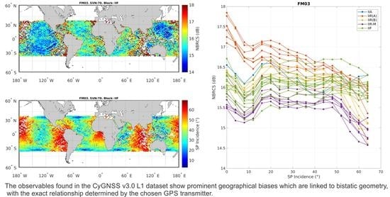
Following the assessment of temporal stability, an assessment of geographical stability was carried out, again at fixed wind speed conditions (U10 ~7 m/s). The analysis presented here considers a single transmitter–receiver pair, but similar results were found using other configurations. Figure 3 top shows a global map of NBRCS reported by the bistatic radar consisting of SVN70 (GPS transmitter) and FM03 (CyGNSS receiver). A well-defined geographical pattern of NBRCS is found around the globe, repeating every 90 degrees in longitude, which cannot be directly attributed to an origin of geophysical nature. A map of the average incidence angle (the vertical angle between the signal path and the line perpendicular to the surface at the specular point) between the transmitter and receiver reveals a similar pattern to NBRCS (Figure 3 bottom). Similar longitudinal NBRCS patterns were found in other transmitter–receiver pairs, albeit varying in magnitude and location. Given the strong correlation between the spatial patterns of NBRCS (Figure 3 top) and the corresponding incidence angle (Figure 3 bottom), it can be speculated that most of the observed NBRCS spatial inhomogeneity can be attributed to the residual dependence of NBRCS on geometry. Thus, further investigation of the relationship between NBRCS and geometry was conducted.
The residual dependence of NBRCS on the incidence angle was examined (Figure 4) for each individual CyGNSS unit and averaged across all GPS transmitters. Overall, as found above, the consistency between different CyGNSS units is good, with similar sensitivity to viewing geometry. However, NBRCS variability with incidence angle exceeds 2 dB, for all CyGNSS receivers. The NBRCS relationship shows a large drop at incidences beyond 50° and a smaller drop is observed in the range of 5°–15°.
Finally, the dependence on the azimuth angle (the angle, in the horizontal plane, of the specular point relative to the receiver’s path of travel) is assessed, with results (Figure 5) showing a non-negligible residual effect in NBRCS of up to ~1 dB for all FMs. In light of these findings, it can be concluded that the observed geographical NBRCS biases can be primarily attributed to residual sensitivity to both azimuth and incidence angle.
3.3. Analysis by GPS Transmitter
Residual dependence on geometry is found to play a prominent role in v3.0 CyGNSS data, with the effect observed to be relatively consistent between receivers (Figure 4). To further understand the geometric dependencies, additional investigations segmented by GPS transmitter (SVN) were performed. Figure 6 shows the dependence of NBRCS estimates on the incidence angle for one CyGNSS receiver (FM03), segmented by individual GPS transmitters (and coloured by the GPS block). At a given wind speed (U10 ~7 m/s), a substantial range (of up to ~3 dB) of NBRCS estimates can be seen between the individual SVNs across 0°–65° incidence.
Further, the dependency on geometry seems to depend on both the individual GPS transmitter and the GPS blocks. More specifically, all SVNs within a given block show a similar relationship with incidence; however, individual SVNs within each block show slight variations around this relationship, as well as overall differences in average NBRCS. This difference between blocks is most marked in Block IIR(A) at incidence angles <30°, where NBRCS estimates can be ~2 dB higher than those found in the other blocks. Additionally, only Block IIF shows approximately constant NBRCS estimates at incidence angles >50°, whereas the other blocks are associated with NBRCS decreases. Significant variability between SVNs is also seen within a given block (up to ~1 dB), which counters the general expectation that similar hardware designs within blocks should lead to similar transmitted power levels at a given geometry.
3.4. Leading Edge Slope (LES)
In addition to NBRCS, the current CyGNSS ocean wind speed retrieval algorithms use a second observable, the LES of the waveform of reflected GPS power. In view of the findings relating to NBRCS, similar investigations of CyGNSS LES data were performed, temporally and in relation to SVN/block and geometry, with very similar results (Appendix A). However, some additional dependencies were found, which are presented here. It needs to be noted that, although the analysis shows LES values converted to dB (i.e., 10 log10), these are not directly representative of any power property and, as such, are not directly comparable to equivalent NBRCS values.
Global maps of LES for a given bistatic configuration show similar geographical patterns as for NBRCS in Figure 4 (not shown). However, the geographical distribution of average LES (Figure 7 top) reported by a single receiver (FM03), averaged across all transmitters, reveals the presence of an additional spatial pattern. Well-defined areas of high and low LES are observed across the global ocean, with differences reaching ~1.5 dB. These patterns show strong resemblance to the contours of the geoid (Figure 7 bottom). This is likely related to how the LES is estimated from the DDMs and suggests that the calculation needs to be further refined in order to prevent the sea surface height from contaminating the LES observable and, subsequently, the L2 ocean wind products.
4. Discussion
4.1. Posting Rate
As was seen in Figure 1, the data posting rate appears to have changed to 2 Hz from July 2019, approximately simultaneously on all CyGNSS satellites (although FM02 appears to change in August, after an earlier abortive attempt in June). It should be noted that this change does not appear to be currently documented, although publications in the literature note the potential that this change offers for improved observations over land waterbodies, e.g., rivers [23], in terms of on-ground resolution. Over ocean, no change is seen in the time-series of average NBRCS at U10 ~7 m/s, although a corresponding change in DDM SNR along with increased NBRCS variability are expected due to the shorter time available for incoherent accumulation of the signal (500 ms).
4.2. Potential Impacts of Observable Biases on Geophysical Retrievals
Large-magnitude deviations are seen in both L1 observables at average ocean wind speed (U10 ~7 m/s), primarily related to changes in viewing geometry, as well as to the GPS transmitter (Figure 4, Figure 5 and Figure 6). However, when looking at global climatologies, the effect of these residual dependencies is likely to be partly obscured due to averaging across the large variability of ocean surface conditions, the number of GPS transmitters, and the number of CyGNSS receivers. However, significant biases are to be expected on shorter spatiotemporal scales, also depending on the transmitter–receiver pair considered. Such L1 deviations are likely to have a significant impact on ocean wind speed retrieval. In particular, given the known inverse relationship between NBRCS and U10 [24], the 3 dB range in NBRCS across geometries is expected to introduce a bias of several m/s already at low-to-moderate wind speeds, with an increasingly stronger impact at higher speeds [21]. The impact on LES is expected to be similar. As such, it is important that steps are taken towards the mitigation of these residual calibration inaccuracies ahead of the release of future versions of the CyGNSS products.
4.3. Potential Origins of Observable Biases
The primary effect on NBRCS and LES is shown to be associated with geometry (Figure 4, Figure 5 and Figure 6), and the primary cause of this likely relates to inaccuracies in the knowledge of antenna gain patterns on both the receiving and transmitting ends. Because of the bistatic nature of the GNSS-R system, two separate antennas are involved in the signal calibration process: one of the two nadir antennas on each CyGNSS receiver, and one from the individual GPS transmitter where the signal originates [25]. The nadir CyGNSS antennas seem to be well inter-calibrated across the constellation, but the consistency of the NBRCS bias pattern might indicate that some of the geometry effect also originates from the receiver end (Figure 4 and Figure 5). It should be noted that the current CyGNSS L2 ocean wind speed algorithm also accounts for the incidence angle [26]; therefore, some of the L1 biases found in this study might well be compensated in the L1-to-L2 inversion process, although L1 data users would need to implement their own corrections prior to inversion. However, calibration inaccuracies originating from differences between individual GPS transmitters appear to dominate (Figure 6). Part of this seems to be related to the GPS block, as similar patterns are seen in each block, which likely relates to differences in antenna design. There is a further component that shows as a bias of up to ~1 dB between individual transmitters within a block (although with a similar relationship with geometry), which likely relates to differences in actual transmit power between the individual SVNs, perhaps due to differences in hardware age.
One additional biasing effect is seen spatially; this, however, is only seen in the LES observable, which shows ~1.5 dB variation linked to mean sea surface height (Figure 7). This is suspected to relate to inaccuracies in the identification of the waveform peak location within the delay Doppler map (DDM).
5. Conclusions
This work provides an assessment of CyGNSS L1 v3.0 products, which have been recently updated to feature a novel calibration approach that includes the capability to exploit data collected from the zenith front-end to account for the variability of available GPS power.
Analysis of the CyGNSS L1 NBRCS shows good temporal stability and negligible inter-receiver and inter-antenna biases, which are constrained to ~0.1 dB and <0.1 dB, respectively. However, prominent geographical biases are found in the global climatologies of NBRCS at given ocean surface conditions. Further examination of the dependence of such biases reveals a strong correlation with viewing geometry, including a marked drop-off at high incidence angles and some variability at lower ones, leading to the observed geographical pattern. Detailed examination of this effect, further segmented by SVN and GPS block, reveals that each block shows different relationships with geometry, with marked biases even between individual SVNs belonging to the same GPS block, indicating the persistence of issues linked to the power calibration of signals originating from different transmitters at different angles.
As current CyGNSS L2 wind products are based on the use of two separate L1 observables (LES and NBRCS), the analysis conducted for NBRCS was extended to LES. The examination of the LES observable led to very similar results as found for NBRCS in terms of temporal stability, inter-FM bias, inter-antenna bias, and dependence on viewing geometry (shown in the Appendix A). However, spatial maps of composite average LES over all bistatic configurations revealed an additional geographical pattern that appears to be correlated with the contours of the geoid. This additional pattern is likely associated with inaccuracies in the current estimation process of the LES of the reflected waveform.
In summary, a number of biases and residual dependencies were found in the latest CyGNSS v3.0 L1 NBRCS and LES products. All appear to be associated with issues either related to unresolved instrument and processing effects or to inaccuracies in the process of direct signal calibration. To avoid such issues in future GNSS-R missions and datasets, particular attention should be given to how bistatic geometry as well as individual GPS transmit powers are handled in the calibration process. Although only ocean-reflected data were analysed here, the calibration effects found in this study are likely to similarly affect land reflections. Given the growing interest in the community in the exploitation of GNSS-R also for land and ice applications, these results highlight the need for further improvements in our understanding of GNSS-R calibration ahead of future releases of the CyGNSS products, as well as in preparation for future missions.
Author Contributions
Methodology and investigations: M.L.H., G.F.; software: M.L.H.; writing—original draft preparation: M.L.H.; writing—review and editing: All; supervision: G.F., C.G., M.S. All authors have read and agreed to the published version of the manuscript.
Funding
This work was funded by ESA contract 4000130560/20/NL/FF/gp.
Institutional Review Board Statement
Not applicable.
Informed Consent Statement
Not applicable.
Data Availability Statement
The ECMWF ERA-5 dataset analyzed in this study is publicly available. This dataset can be found at: https://cds.climate.copernicus.eu/cdsapp#!/dataset/reanalysis-era5-single-levels?tab=overview (accessed on 20 August 2021). The CyGNSS v3.0 L1 dataset can be found at: https://podaac.jpl.nasa.gov/dataset/CYGNSS_L1_V3.0 (accessed on 20 August 2021).
Acknowledgments
ERA-5 data were generated using Copernicus Climate Change Service Information (2021); neither the European Commission nor ECMWF is responsible for any use that may be made of the Copernicus Information or the data it contains. CyGNSS data can be publicly downloaded from the NASA PO.DAAC.
Conflicts of Interest
The authors declare no conflict of interest.
Appendix A
Figure A1.
Temporal evolution of leading edge slope (LES) estimates at U10 ~7 m/s, for all SVNs, segmented by CyGNSS Flight Model (FM01-FM08).
Figure A1.
Temporal evolution of leading edge slope (LES) estimates at U10 ~7 m/s, for all SVNs, segmented by CyGNSS Flight Model (FM01-FM08).

Figure A2.
Dependence of LES on incidence angle (from nadir 0° to 65°) at U10 ~7 m/s, for all SVNs, segmented by CyGNSS Flight Model (FM01-FM08).
Figure A2.
Dependence of LES on incidence angle (from nadir 0° to 65°) at U10 ~7 m/s, for all SVNs, segmented by CyGNSS Flight Model (FM01-FM08).

Figure A3.
Dependence of leading edge slope (LES) on azimuth, segmented by CyGNSS receiver (FM01-FM08), at U10 ~7 m/s, for all SVNs, from the starboard (left panel) and port (right panel) nadir antennas.
Figure A3.
Dependence of leading edge slope (LES) on azimuth, segmented by CyGNSS receiver (FM01-FM08), at U10 ~7 m/s, for all SVNs, from the starboard (left panel) and port (right panel) nadir antennas.

Figure A4.
Dependence of LES on incidence angle, at U10 ~7 m/s, from CyGNSS FM03, segmented by SVN and coloured by GPS block.
Figure A4.
Dependence of LES on incidence angle, at U10 ~7 m/s, from CyGNSS FM03, segmented by SVN and coloured by GPS block.

References
- Hall, C.D.; Cordey, R.A. Multistatic Scatterometry. In Proceedings of the International Geoscience and Remote Sensing Symposium, ’Remote Sensing: Moving toward the 21st Century, Edinburgh, UK, 12–16 September 1988; pp. 561–562. [Google Scholar]
- Martin-Neira, M. A passive reflectometry and interferometry system (PARIS): Application to ocean altimetry. ESA J. 1993, 17, 331–355. [Google Scholar]
- Gleason, S.; Hodgart, S.; Sun, Y.; Gommenginger, C.; Mackin, S.; Adjrad, M. Detection and Processing of Bistatically Reflected GPS Signals from Low Earth Orbit for the Purpose of Ocean Remote Sensing. IEEE Trans. Geosci. Remote Sens. 2005, 43, 1229–1241. [Google Scholar] [CrossRef] [Green Version]
- Foti, G.; Gommenginger, C.; Jales, P.; Unwin, M.; Shaw, A.; Robertson, C.; Rosello, J. Spaceborne GNSS reflectometry for ocean winds: First results from the UK TechDemoSat-1 mission. Geophys. Res. Lett. 2015, 42, 5435–5441. [Google Scholar] [CrossRef] [Green Version]
- Unwin, M.; Jales, P.; Tye, J.; Gommenginger, C.; Foti, G.; Rosello, J. Spaceborne GNSS-Reflectometry on TechDemoSat-1: Early Mission Operations and Exploitation. IEEE J. Sel. Top. Appl. Earth Obs. Remote Sens. 2016, 9, 4525–4539. [Google Scholar] [CrossRef]
- Ruf, C.S.; Chew, C.; Lang, T.; Morris, M.G.; Nave, K.; Ridley, A.; Balasubramaniam, R. A New Paradigm in Earth Environmental Monitoring with the CYGNSS Small Satellite Constellation. Sci. Rep. 2018, 8, 8782. [Google Scholar] [CrossRef] [PubMed] [Green Version]
- Soisuvarn, S.; Jelenak, Z.; Said, F.; Chang, P.S.; Egido, A. The GNSS Reflectometry Response to the Ocean Surface Winds and Waves. IEEE J. Sel. Top. Appl. Earth Obs. Remote Sens. 2016, 9, 4678–4699. [Google Scholar] [CrossRef]
- Foti, G.; Gommenginger, C.; Srokosz, M. First Spaceborne GNSS-Reflectometry Observations of Hurricanes From the UK TechDemoSat-1 Mission. Geophys. Res. Lett. 2017, 44, 12358–12366. [Google Scholar] [CrossRef] [Green Version]
- Ruf, C.; Asharaf, S.; Balasubramaniam, R.; Gleason, S.; Lang, T.; McKague, D.; Twigg, D.; Waliser, D. In-Orbit Performance of the Constellation of CyGNSS Hurricane Satellites. Am. Meteorol. Soc. 2019, 100, 2009–2023. [Google Scholar] [CrossRef]
- Cartwright, J.; Banks, C.J.; Srokosz, M. Sea Ice Detection Using GNSS-R Data From TechDemoSat-1. J. Geophys. Res. Ocean. 2019, 124, 5801–5810. [Google Scholar] [CrossRef]
- Chew, C.C.; Small, E.E. Soil Moisture Sensing Using Spaceborne GNSS Reflections: Comparison of CyGNSS Reflectivity to SMAP Soil Moisture. Geophys. Res. Lett. 2018, 45, 4049–4057. [Google Scholar] [CrossRef] [Green Version]
- Zavorotny, V.U.; Gleason, S.; Cardellach, E.; Camps, A. Tutorial on remote sensing using GNSS bistatic radar of opportunity. IEEE Geosci. Remote Sens. Mag. 2014, 2, 8–45. [Google Scholar] [CrossRef] [Green Version]
- Ruf, C.; Gleason, S.; Jelenak, Z.; Katzberg, S.; Ridley, S.; Rose, R.; Scherrer, J.; Zavorotny, V. The NASA EV-2 Cyclone Global Navigation Satellite System (CyGNSS) mission. In Proceedings of the 2013 IEEE Aerospace Conference, Big Sky, MT, USA, 2–9 March 2013; pp. 1–7. [Google Scholar]
- Chew, C.; Reager, J.T.; Small, E. CyGNSS data map flood inundation during the 2017 Atlantic hurricane season. Sci. Rep. 2018, 8, 9336. [Google Scholar] [CrossRef] [PubMed]
- Saïd, F.; Jelenak, Z.; Park, J.; Chang, P.S. The NOAA Track-Wise Wind Retrieval Algorithm and Product Assessment for CyGNSS. IEEE Trans. Geosci. Remote Sens. 2021, 1–24. [Google Scholar] [CrossRef]
- Wang, T.; Ruf, C.; Gleason, S.; Block, B.; Mckague, D.; Brien, A.O. A Real-Time EIRP Level 1 Calibration Algorithm for the CYGNSS Mission Using the Zenith Measurements. In Proceedings of the IGARSS 2019—2019 IEEE International Geoscience and Remote Sensing Symposium, Yokohama, Japan, 28 July–2 August 2019; pp. 8725–8728. [Google Scholar] [CrossRef]
- Wang, T.; Ruf, C.; Block, B.; McKague, D. Characterization of the Transmit Power and Antenna Pattern of the GPS Constellation for the CYGNSS Mission. In Proceedings of the IGARSS 2018—2018 IEEE International Geoscience and Remote Sensing Symposium, Valencia, Spain, 22–27 July 2018; pp. 4011–4014. [Google Scholar]
- Gleason, S. Level 1B DDM Calibration Algorithm Theoretical Basis Document rev. 3, CyGNSS Project Document 148-0137. Available online: https://podaac-tools.jpl.nasa.gov/drive/files/allData/cygnss/L1/docs/148-0137-3_ATBD_L1B_v3.0_DDMCalibration_Release.pdf (accessed on 20 August 2021).
- Hersbach, H.; De Rosnay, P.; Bell, B.; Schepers, D.; Simmons, A.; Soci, C.; Abdalla, S.; Balmaseda, A.; Balsamo, G.; Bechtold, P.; et al. Operational Global Reanalysis: Progress, Future Directions and Synergies with NWP Including Updates on the ERA5 Production Status. Available online: https://www.ecmwf.int/en/elibrary/18765-operational-global-reanalysis-progress-future-directions-and-synergies-nwp (accessed on 20 August 2021).
- Belmonte Rivas, M.; Stoffelen, A. Characterizing ERA-interim and ERA5 surface wind biases using ASCAT. Ocean Sci. 2019, 15, 831–852. [Google Scholar] [CrossRef] [Green Version]
- Said, F.; Jelenak, Z.; Chang, P.S.; Soisuvarn, S. An Assessment of CYGNSS Normalized Bistatic Radar Cross Section Calibration. IEEE J. Sel. Top. Appl. Earth Obs. Remote Sens. 2019, 12, 50–65. [Google Scholar] [CrossRef]
- Pavlis, N.K.; Holmes, S.A.; Kenyon, S.C.; Factor, J.K. The development and evaluation of the Earth Gravitational Model 2008 (EGM2008). J. Geophys. Res. Solid Earth 2012, 117, 1–38. [Google Scholar] [CrossRef] [Green Version]
- Gleason, S.; Brien, A.O.; Russel, A.; Al-khaldi, M.M.; Johnson, J.T. Geolocation, Calibration and Surface Resolution of CyGNSS GNSS-R Land Observations. Remote Sens. 2020, 12, 1317. [Google Scholar] [CrossRef] [Green Version]
- Ruf, C.S.; Balasubramaniam, R.; Member, S. Development of the CYGNSS Geophysical Model Function for Wind Speed. IEEE J. Sel. Top. Appl. Earth Obs. Remote Sens. 2019, 12, 66–77. [Google Scholar] [CrossRef]
- Zavorotny, V.U.; Voronovich, A.G. Scattering of GPS Signals from the Ocean with Wind Remote Sensing Application. IEEE Trans. Geosci. Remote Sens. 2000, 38, 951–964. [Google Scholar] [CrossRef] [Green Version]
- Clarizia, M.P.; Zavorotny, V.; Ruf, C. Level 2 Wind Speed Retrieval Algorithm Theoretical Basis Document rev. 6, CyGNSS Project Document 148-0138. Available online: https://podaac-tools.jpl.nasa.gov/drive/files/allData/cygnss/L2/docs/148-0138-6_ATBD_L2_v3.0_Wind_Speed_Retrieval.pdf (accessed on 20 August 2021).
Figure 1.
Temporal availability of CyGNSS records by flight model (FM01-FM08).

Figure 2.
Temporal evolution of NBRCS estimates at ERA5 U10 ~7 m/s for all SVNs, segmented by CyGNSS Flight Model (FM01-FM08).
Figure 2.
Temporal evolution of NBRCS estimates at ERA5 U10 ~7 m/s for all SVNs, segmented by CyGNSS Flight Model (FM01-FM08).

Figure 3.
(top) Geographical distribution of NBRCS reported by CyGNSS FM03 for signals incoming from GPS SVN70 (Block IIF) for U10 ~7 m/s. (bottom) Corresponding geographical distribution of incidence angle between CyGNSS FM03 and GPS SVN70 (Block IIF).
Figure 3.
(top) Geographical distribution of NBRCS reported by CyGNSS FM03 for signals incoming from GPS SVN70 (Block IIF) for U10 ~7 m/s. (bottom) Corresponding geographical distribution of incidence angle between CyGNSS FM03 and GPS SVN70 (Block IIF).

Figure 4.
Dependence of NBRCS on incidence angle (from nadir 0° to 65°) at U10 ~7 m/s, averaged for all GPS transmitters/SVNs; each line (and colour) represents a different CyGNSS Flight Model/receiver (FM01-FM08).
Figure 4.
Dependence of NBRCS on incidence angle (from nadir 0° to 65°) at U10 ~7 m/s, averaged for all GPS transmitters/SVNs; each line (and colour) represents a different CyGNSS Flight Model/receiver (FM01-FM08).

Figure 5.
Dependence of NBRCS on azimuth at ERA-5 U10 ~7 m/s, for all GPS transmitters/SVNs, segmented by CyGNSS Flight Models (FM01-FM08).
Figure 5.
Dependence of NBRCS on azimuth at ERA-5 U10 ~7 m/s, for all GPS transmitters/SVNs, segmented by CyGNSS Flight Models (FM01-FM08).

Figure 6.
Residual dependence of NBRCS reported by CyGNSS FM03 at U10 ~7 m/s on incidence angle; each line represents a different GPS transmitter/SVN and is coloured by the GPS block to which the transmitter belongs.
Figure 6.
Residual dependence of NBRCS reported by CyGNSS FM03 at U10 ~7 m/s on incidence angle; each line represents a different GPS transmitter/SVN and is coloured by the GPS block to which the transmitter belongs.

Figure 7.
(top) Geographical distribution of leading edge slope (LES) at U10 ~7 m/s reported by FM03 averaged across all SVNs over August 2018–December 2019; (bottom) global map of geoid (EGM 2008) [22].
Figure 7.
(top) Geographical distribution of leading edge slope (LES) at U10 ~7 m/s reported by FM03 averaged across all SVNs over August 2018–December 2019; (bottom) global map of geoid (EGM 2008) [22].

Publisher’s Note: MDPI stays neutral with regard to jurisdictional claims in published maps and institutional affiliations. |
© 2021 by the authors. Licensee MDPI, Basel, Switzerland. This article is an open access article distributed under the terms and conditions of the Creative Commons Attribution (CC BY) license (https://creativecommons.org/licenses/by/4.0/).
Share and Cite
MDPI and ACS Style
Hammond, M.L.; Foti, G.; Gommenginger, C.; Srokosz, M. An Assessment of CyGNSS v3.0 Level 1 Observables over the Ocean. Remote Sens. 2021, 13, 3500. https://doi.org/10.3390/rs13173500
AMA Style
Hammond ML, Foti G, Gommenginger C, Srokosz M. An Assessment of CyGNSS v3.0 Level 1 Observables over the Ocean. Remote Sensing. 2021; 13(17):3500. https://doi.org/10.3390/rs13173500
Chicago/Turabian StyleHammond, Matthew Lee, Giuseppe Foti, Christine Gommenginger, and Meric Srokosz. 2021. "An Assessment of CyGNSS v3.0 Level 1 Observables over the Ocean" Remote Sensing 13, no. 17: 3500. https://doi.org/10.3390/rs13173500
Note that from the first issue of 2016, this journal uses article numbers instead of page numbers. See further details here.