Inter-Algorithm Relationships for the Estimation of the Fraction of Vegetation Cover Based on a Two Endmember Linear Mixture Model with the VI Constraint


Abstract
:1. Introduction
2. Model Assumptions and Retrieval Algorithms
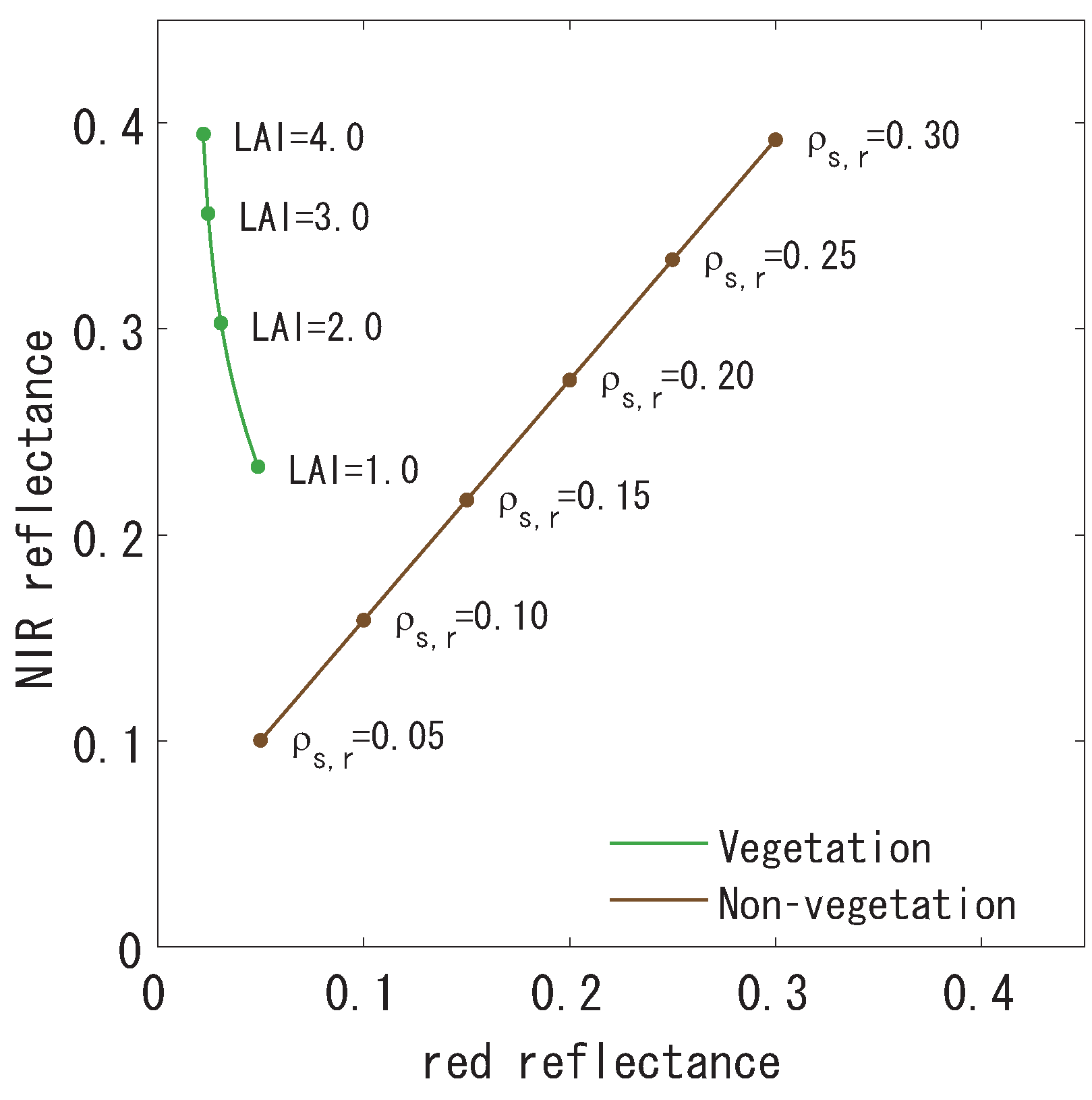
2.1. Model Assumptions
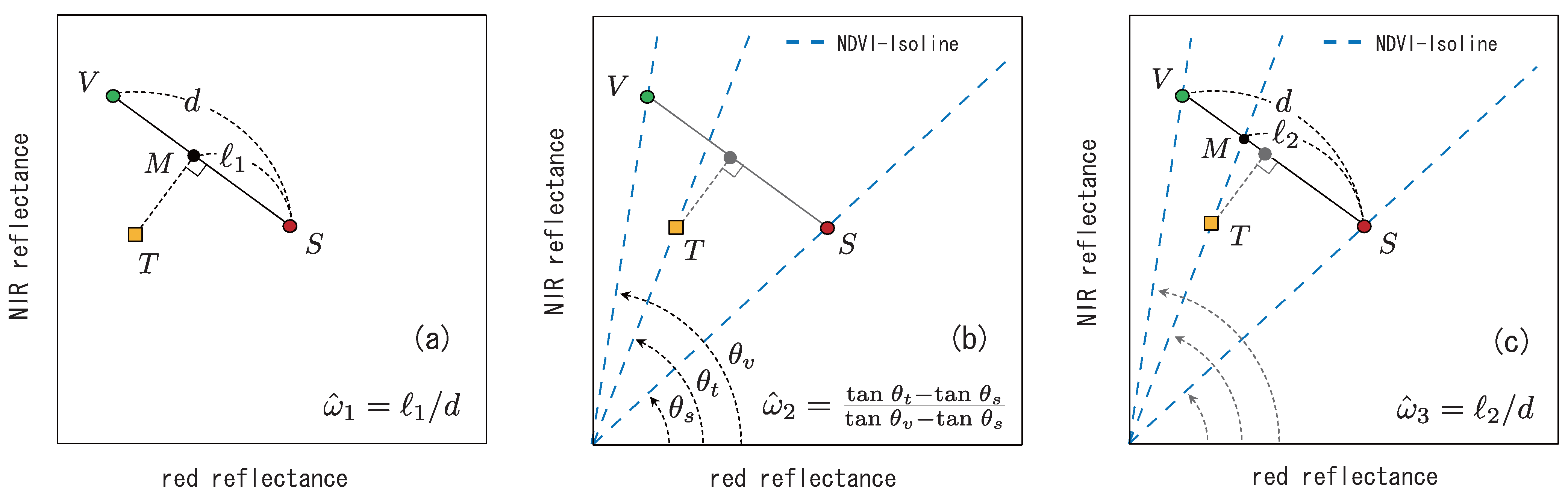
2.2. Algorithm-1: Reflectance-Based LMM
2.3. Algorithm-2: VI-Based LMM

| NDVI | 1 | 0 | 1 | 1 | 0 | |
| DVI | 1 | 0 | 0 | 0 | 1 | |
| PVI | 1 | 0 | 0 | |||
| SAVI | 0 | 1 | 1 | |||
| TSAVI | a | 1 | a | |||
| EVI2 | 0 | 1 | 1 |
2.4. Algorithm-3: VI-Isoline-Based LMM
3. Relationships Among the Algorithms
3.1. Relationships Between Algorithm-1 and the Others
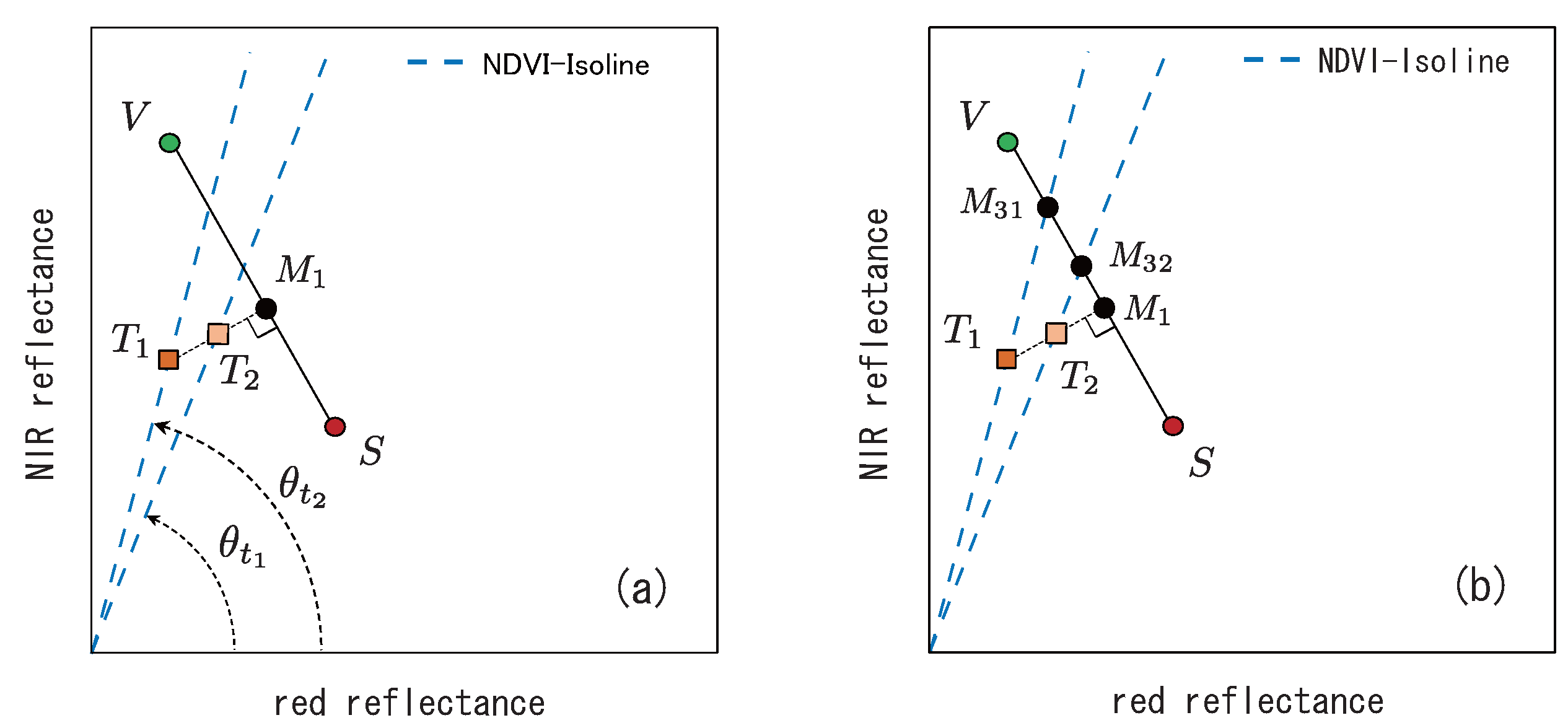
3.2. Relationship Between Algorithms-2 and -3
| NDVI | ||
| DVI | 0 | |
| PVI | 0 | |
| SAVI | ||
| TSAVI | ||
| EVI2 |
4. Numerical Results
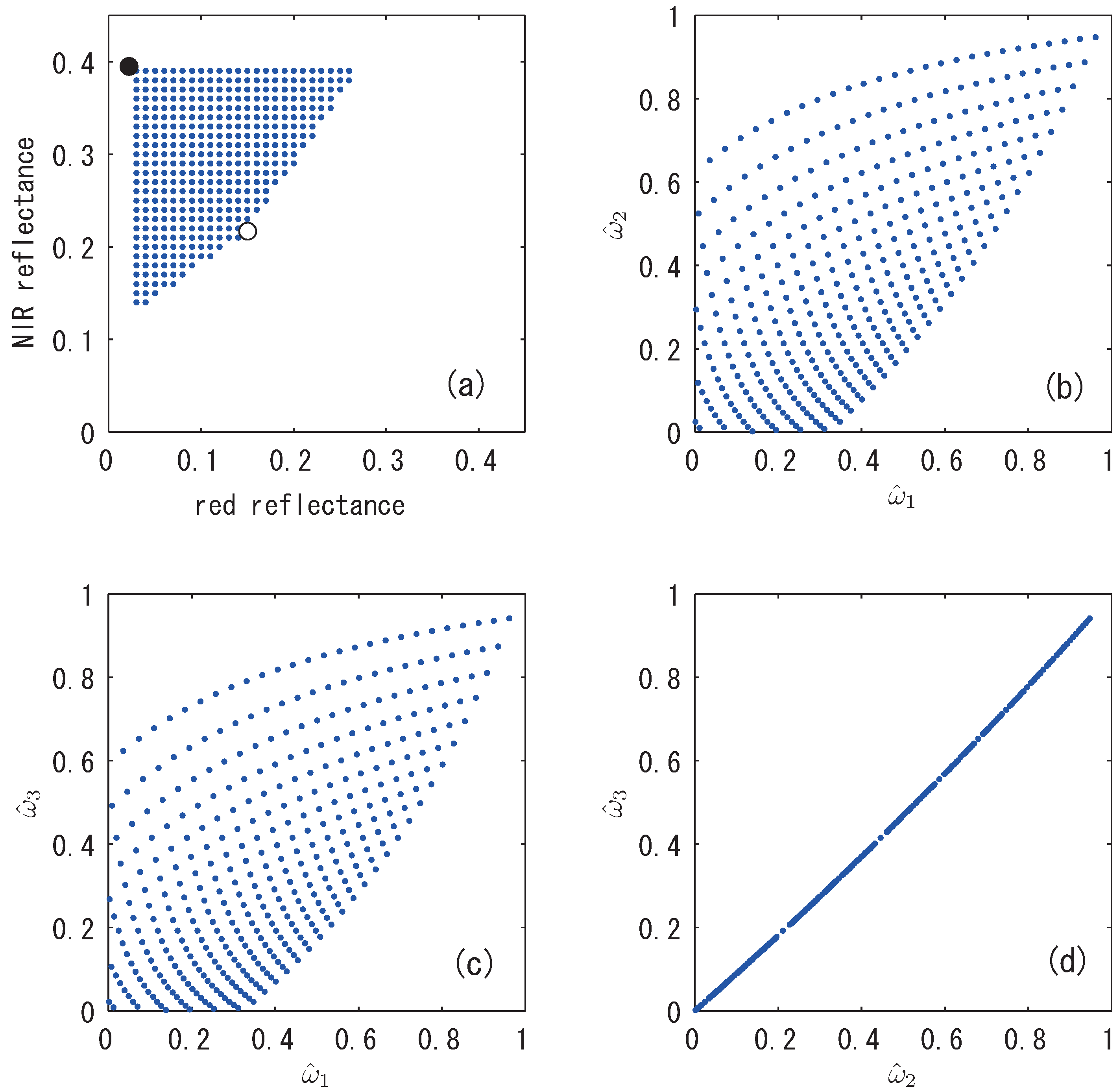
4.1. Uncertainties in the Relationships
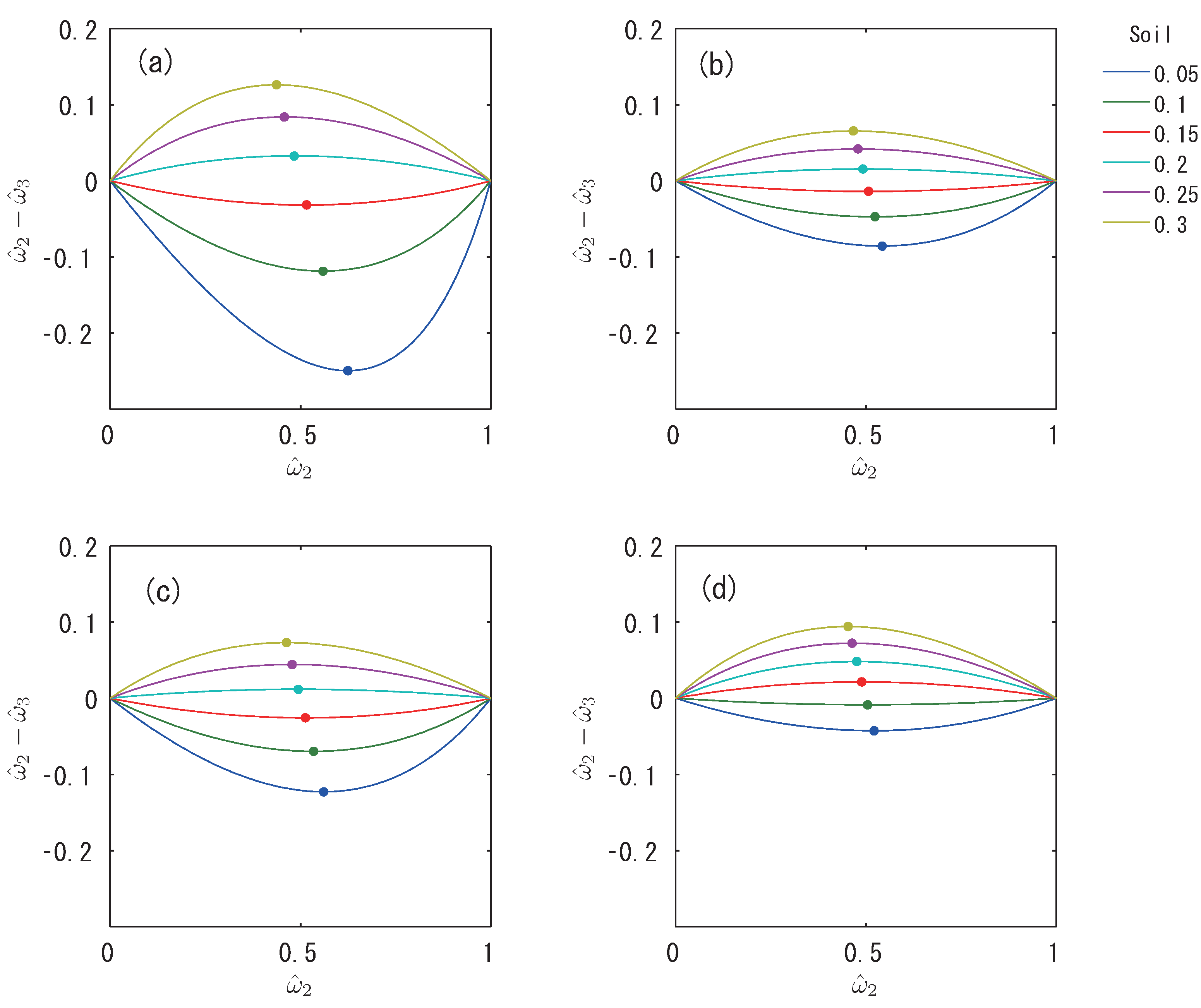
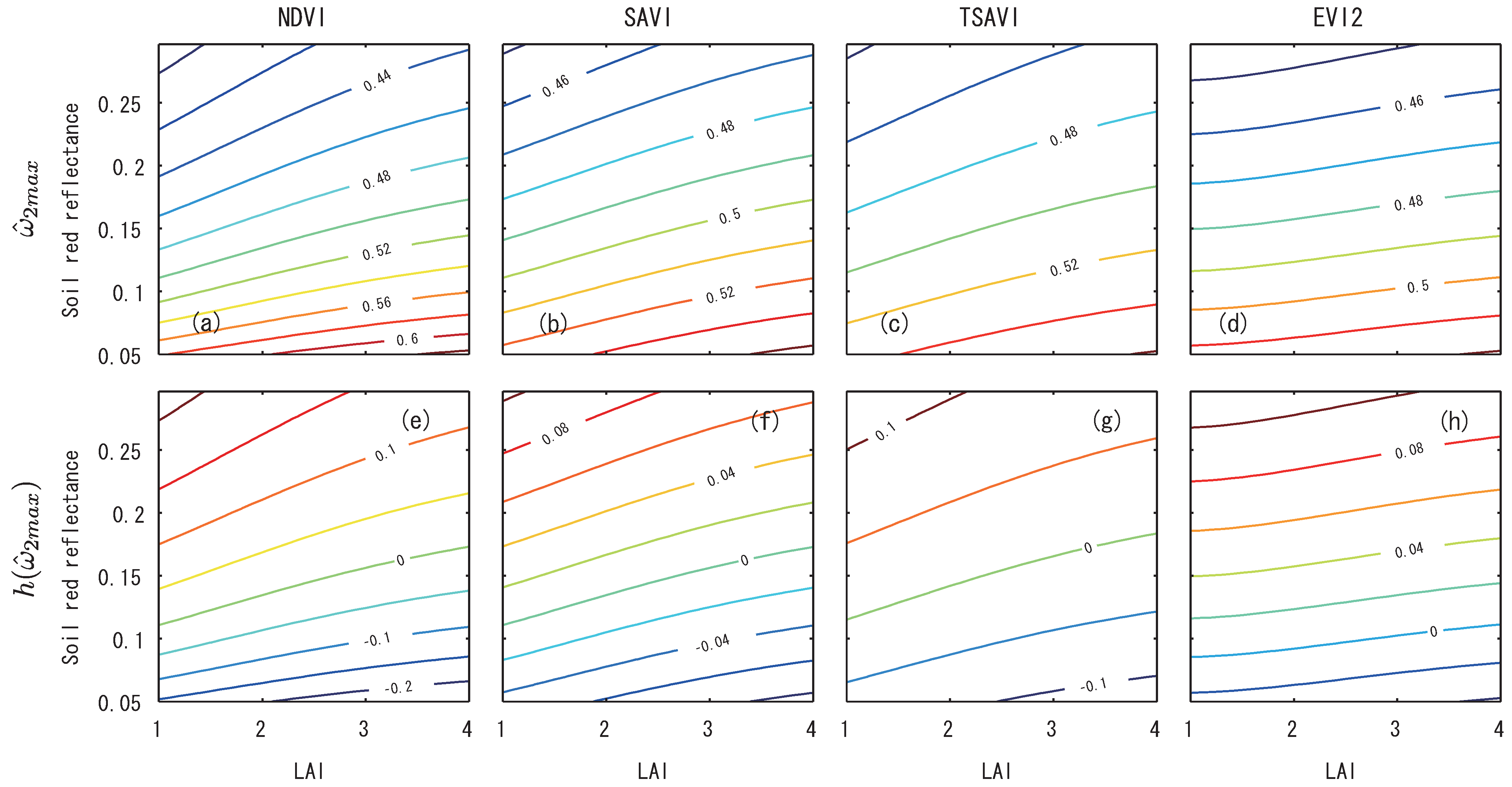
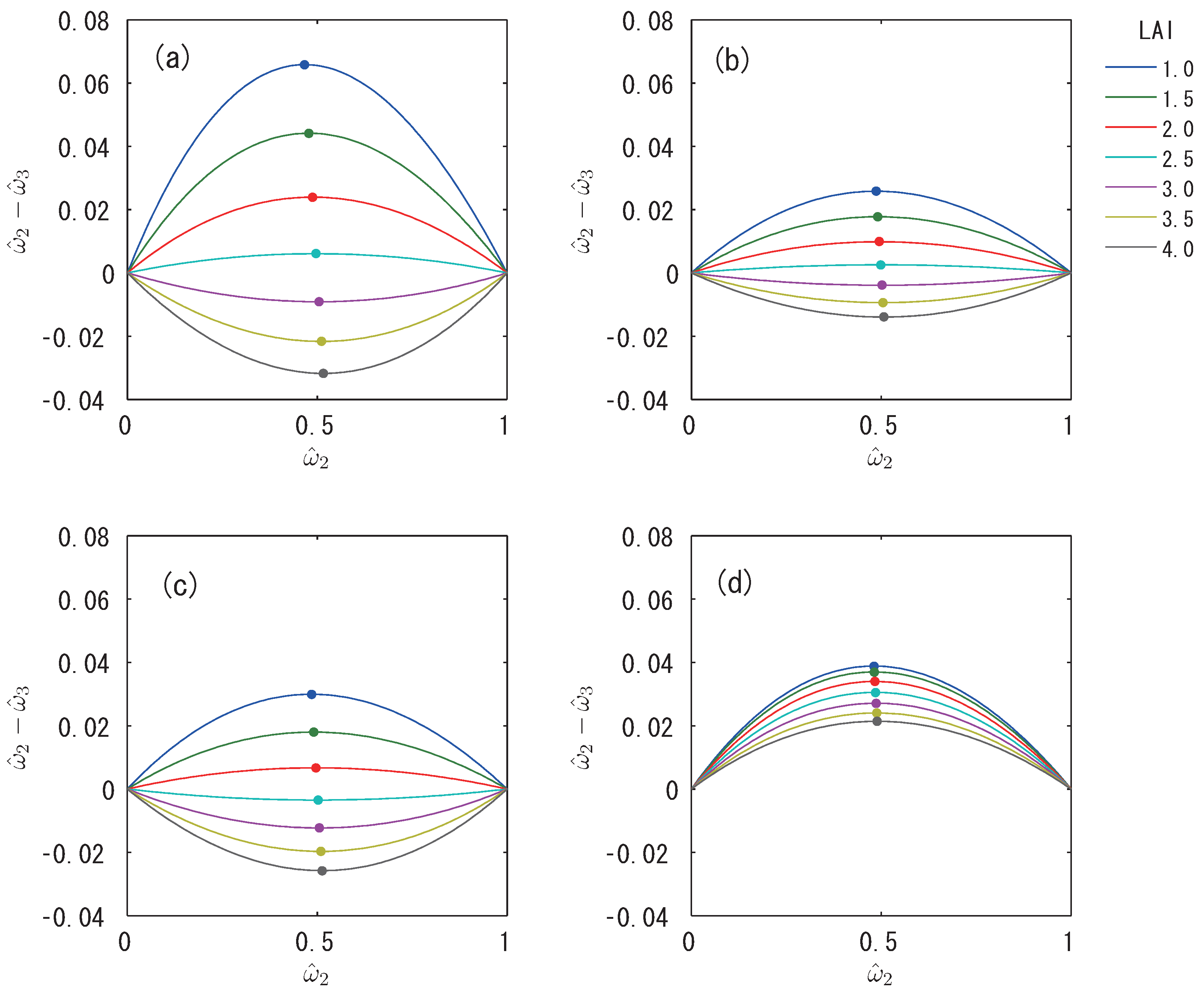
4.2. Differences Between and as a Function of Endmember Spectra


4.3. The Maximum Difference Between and

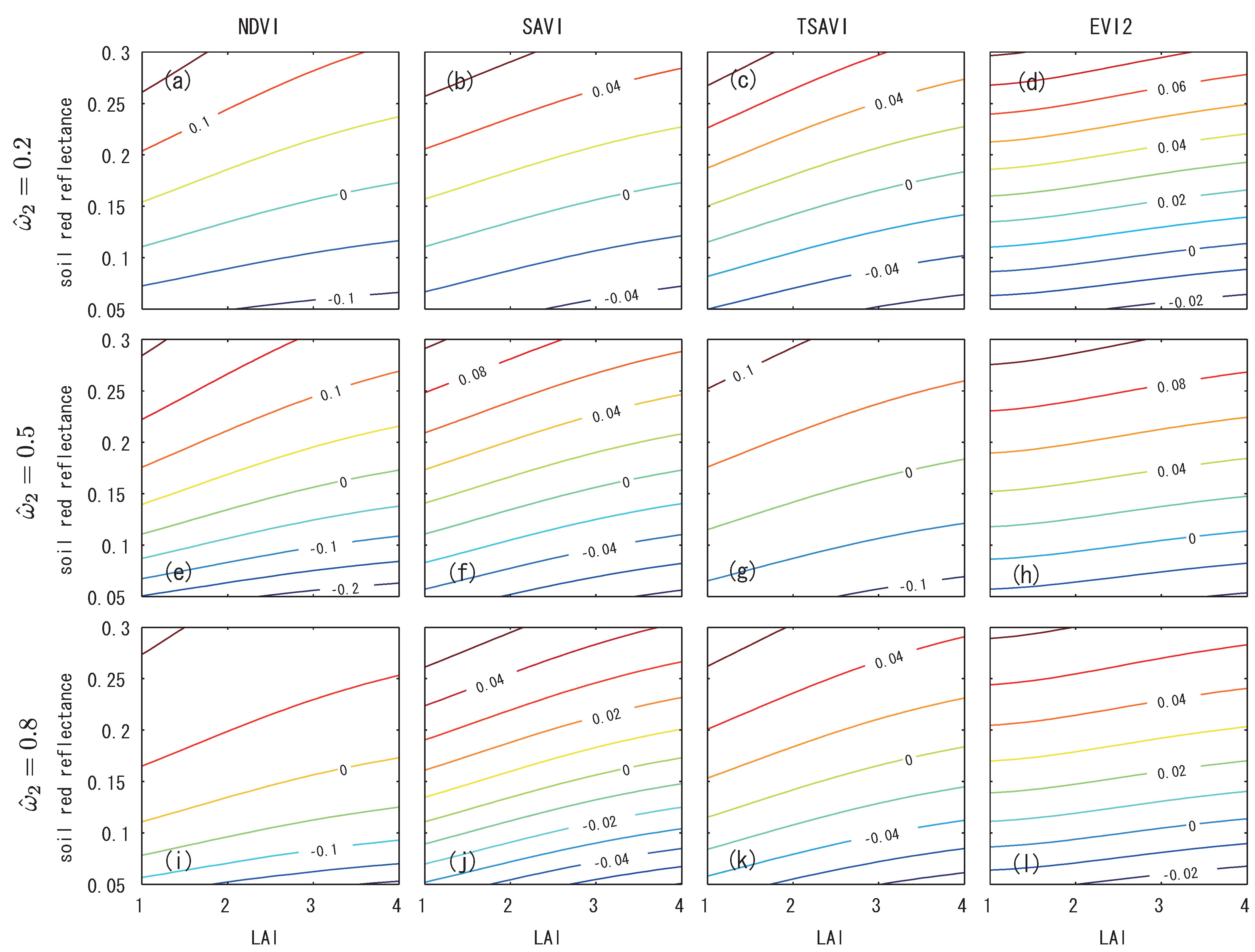
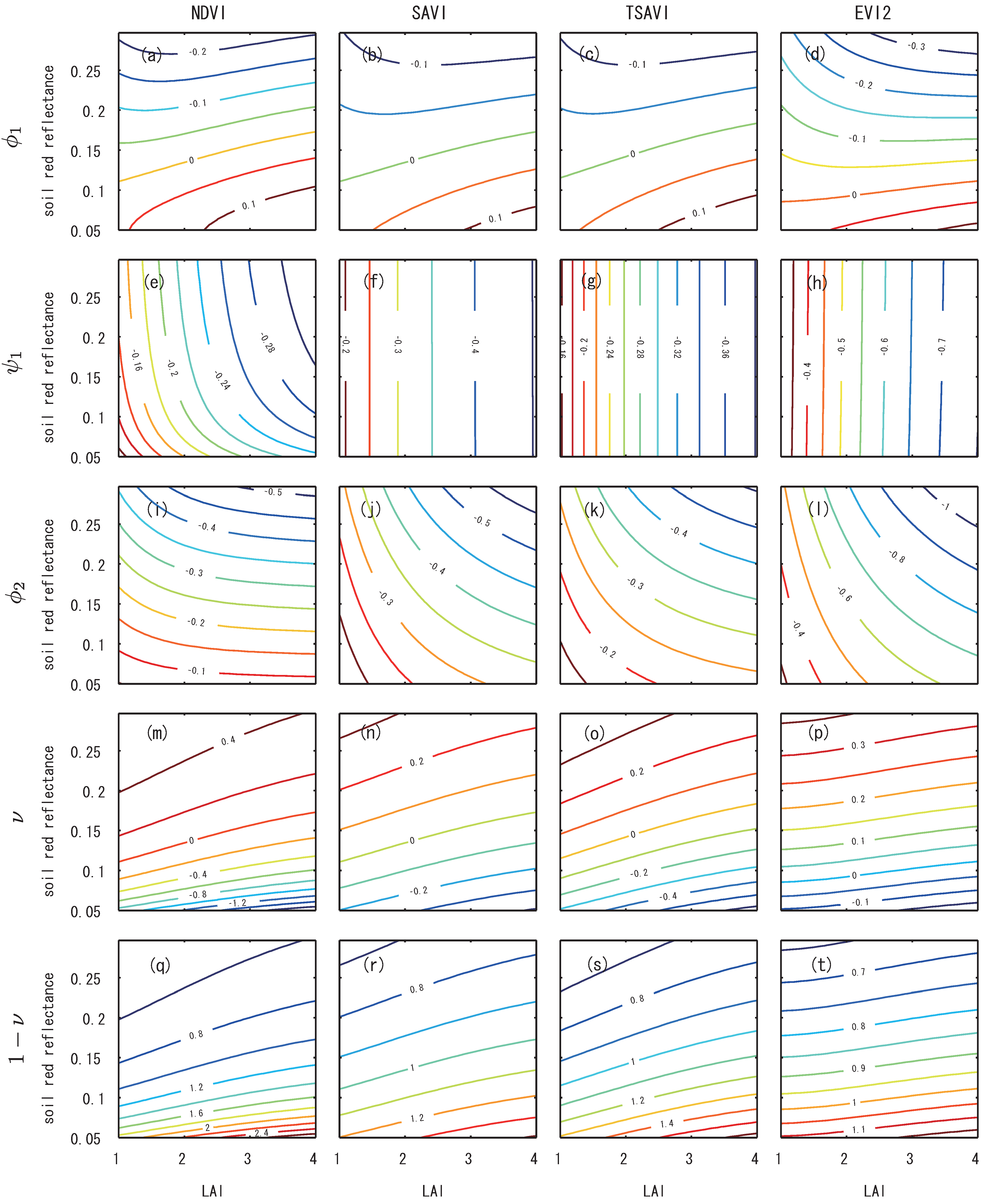
4.4. Variations of ν, , , and with Variations in the Endmember Spectra

5. Discussion
Acknowledgements
References
- Lu, H.; Raupach, M.R.; McVicar, T.R. Decomposition of Vegetation Cover into Woody and Herbaceous Components Using AVHRR NDVI Time Series; Technical Report 35/01; CSIRO Land and Water: Canberra, Australia, 2001. [Google Scholar]
- Jiang, Z.; Huete, A.R.; Chen, J.; Chen, Y.; Li, J.; Yan, G.; Zhang, X. Analysis of NDVI and scaled difference vegetation index retrievals of vegetation fraction. Remote Sens. Environ. 2006, 101, 366–378. [Google Scholar] [CrossRef]
- Aman, A.; Randriamanantena, H.P.; Podaire, A.; Frouin, R. Upscale integration of normalized difference vegetation index: The problem of spatial heterogeneity. IEEE Trans. Geosci. Remote Sens. 1992, 30, 326–338. [Google Scholar] [CrossRef]
- Jimenéz-Muñoz, J.C.; Sobrino, J.A.; Plaza, A.; Guanter, L.; Moreno, J.; Martinez, P. Comparison between fractional vegetation cover retrievals from vegetation indices and spectral mixture analysis: Case study of PROBA/CHRIS data over an agricultural area. Sensors 2009, 9, 768–793. [Google Scholar] [CrossRef] [PubMed]
- Song, C. Spectral mixture analysis for subpixel vegetation fractions in the urban environment: How to incorporate endmember variability? Remote Sens. Environ. 2005, 95, 248–263. [Google Scholar] [CrossRef]
- Asner, G.P. Biophysical and biochemical sources of variability in canopy reflectance. Remote Sens. Environ. 1998, 64, 234–253. [Google Scholar] [CrossRef]
- Gutman, G.; Ignatov, A. The derivation of the green vegetation fraction from NOAA/AVHRR data for use in numerical weather prediction models. Int. J. Remote Sens. 1998, 19, 1533–1543. [Google Scholar] [CrossRef]
- Lobell, D.B.; Asner, G.P.; Law, B.E.; Treuhaft, R.N. Subpixel canopy cover estimation of coniferous forests in Oregon using SWIR imaging spectrometry. J. Geophys. Res. 2001, 106, 5151–5160. [Google Scholar] [CrossRef]
- Lu, D.; Moran, E.; Batistella, M. Linear mixture model applied to Amazonian vegetation classification. Remote Sens. Environ. 2003, 87, 456–469. [Google Scholar] [CrossRef]
- Braswell, B.H.; Hagen, S.C.; Frolking, S.E.; Salas, W.A. A multivariable approach for mapping sub-pixel land cover distributions using MISR and MODIS: Application in the Brazilian Amazon region. Remote Sens. Environ. 2003, 87, 243–256. [Google Scholar] [CrossRef]
- Weng, Q.; Lu, D.; Schubring, J. Estimation of land surface temperature-vegetation abundance relationship for urban heat island studies. Remote Sens. Environ. 2004, 89, 467–483. [Google Scholar] [CrossRef]
- Weng, Q.; Lu, D. A sub-pixel analysis of urbanization effect on land surface temperature and its interplay with impervious surface and vegetation coverage in Indianapolis, United States. Int. J. Appl. Earth Obs. Geoinf. 2008, 10, 68–83. [Google Scholar] [CrossRef]
- Shimabukuro, Y.E.; Smith, J.A. The least-squares mixing models to generate fraction images derived from remote sensing multispectral data. IEEE Trans. Geosci. Remote Sens. 1991, 29, 16–20. [Google Scholar] [CrossRef]
- Xiao, J.; Moody, A. A comparison of methods for estimating fractional green vegetation cover within a desert-to-upland transition zone in central New Mexico, USA. Remote Sens. Environ. 2005, 98, 237–250. [Google Scholar] [CrossRef]
- Jasinski, M.F.; Eagleson, P.S. Estimation of subpixel vegetation cover using red-infrared scattergrams. IEEE Trans. Geosci. Remote Sens. 1990, 28, 253–267. [Google Scholar] [CrossRef]
- Jasinski, M.F. Estimation of subpixel vegetation density of natural regions using satellite multispectral imagery. IEEE Trans. Geosci. Remote Sens. 1996, 34, 804–813. [Google Scholar] [CrossRef]
- Huemmrich, K.F. The GeoSail model: A simple addition to the SAIL model to describe discontinuous canopy reflectance. Remote Sens. Environ. 2001, 75, 423–431. [Google Scholar] [CrossRef]
- Carpenter, G.A.; Gopal, S.; Macomber, S.; Martens, S.; Woodcock, C.E. A neural network method for mixture estimation for vegetation mapping. Remote Sens. Environ. 1999, 70, 138–152. [Google Scholar] [CrossRef]
- Guilfoyle, K.J.; Althouse, M.L.; Chang, C.-I. A quantitative and comparative analysis of linear and nonlinear spectral mixture models using radial basis function neural networks. IEEE Trans. Geosci. Remote Sens. 2001, 39, 2314–2318. [Google Scholar] [CrossRef]
- Adams, J.B.; Smith, M.O.; Johnson, P.E. Spectral mixture modeling: a new analysis of rock and soil types at the Viking Lander 1 site. J. Geophys. Res. 1986, 91, 8098–8112. [Google Scholar] [CrossRef]
- Settle, J.J.; Drake, N.A. Linear mixing and the estimation of ground cover proportions. Int. J. Remote Sens. 1993, 14, 1159–1177. [Google Scholar] [CrossRef]
- Foody, G.M.; Cox, D.P. Sub-pixel land cover composition estimation using a linear mixture model and fuzzy membership functions. Int. J. Remote Sens. 1994, 15, 619–631. [Google Scholar] [CrossRef]
- Ichoku, C.; Karnieli, A. A review of mixture modeling techniques for sub-pixel land cover estimation. Remote Sens. Rev. 1996, 13, 161–186. [Google Scholar] [CrossRef]
- García-Haro, F.J.; Gilbert, M.A.; Meliá, J. Linear spectral mixture modelling to estimate vegetation amount from optical spectral data. Int. J. Remote Sens. 1996, 17, 3373–3400. [Google Scholar] [CrossRef]
- Zeng, X.; Dickinson, R.E.; Walker, A.; Shaikh, M.; Defries, R.S.; Qi, J. Derivation and evaluation of global 1-km fractional vegetation cover data for land modeling. J. Appl. Meteorol. 2000, 39, 826–839. [Google Scholar] [CrossRef]
- Hirano, Y.; Yasuoka, Y.; Shibasaki, R. Pragmatic approach for estimation of vegetation cover ratio in urban area using NDVI. J. Jpn. Soc. Remote Sens. (in Japanese with English abstract) 2002, 22, 163–174. [Google Scholar]
- Haertel, V.F.; Shimabukuro, Y.E. Spectral linear mixing model in low spatial resolution image data. IEEE Trans. Geosci. Remote Sens. 2005, 43, 2555–2562. [Google Scholar] [CrossRef]
- Pu, R.; Gong, P.; Michishita, R.; Sasagawa, T. Spectral mixture analysis for mapping abundance of urban surface components from the Terra/ASTER data. Remote Sens. Environ. 2008, 112, 939–954. [Google Scholar] [CrossRef]
- Hestir, E.L.; Khanna, S.; Andrew, M.E.; Santos, M.J.; Viers, J.H.; Greenberg, J.A.; Rajapakse, S.S.; Ustin, S.L. Identification of invasive vegetation using hyperspectral remote sensing in the California Delta ecosystem. Remote Sens. Environ. 2008, 112, 4034–4047. [Google Scholar] [CrossRef]
- Zhang, J.; Rivard, B.; Rogge, D.M. The successive projection algorithm (SPA), an algorithm with a spatial constraint for the automatic search of endmembers in hyperspectral Data. Sensors 2008, 8, 1321–1342. [Google Scholar] [CrossRef]
- Chen, J.; Jia, X.; Yang, W.; Matsushita, B. Generalization of subpixel analysis for hyperspectral data with flexibility in spectral similarity measures. IEEE Trans. Geosci. Remote Sens. 2009, 47, 2165–2171. [Google Scholar] [CrossRef]
- Small, C. Estimation of urban vegetation abundance by spectral mixture analysis. Int. J. Remote Sens. 2001, 22, 1305–1334. [Google Scholar] [CrossRef]
- Chang, C.I.; Ren, H.; Chang, C.C.; D’Amico, F.; Jensen, J.O. Estimation of subpixel target size for remotely sensed imagery. IEEE Trans. Geosci. Remote Sens. 2004, 42, 1309–1320. [Google Scholar] [CrossRef]
- Van de Voorde, T.; Vlaeminck, J.; Canters, F. Comparing different approaches for mapping urban vegetation cover from landsat ETM+ data: A case study on Brussels. Sensors 2008, 8, 3880–3902. [Google Scholar] [CrossRef]
- Cavalli, R.M.; Pascucci, S.; Pignatti, S. Optimal spectral domain selection for maximizing archaeological signatures: Italy case studies. Sensors 2009, 9, 1754–1767. [Google Scholar] [CrossRef] [PubMed]
- Wittich, K.P.; Hausing, O. Area-averaged vegetative cover fraction estimated from satellite data. Int. J. Biometeorol. 1995, 38, 209–215. [Google Scholar] [CrossRef]
- Carlson, T.N.; Ripley, D.A. On the relation between NDVI, fractional vegetation cover, and leaf area index. Remote Sens. Environ. 1997, 62, 241–252. [Google Scholar] [CrossRef]
- Carlson, T.N.; Arthur, S.T. The impact of land use-land cover changes due to urbanization on surface microclimate and hydrology: A satellite perspective. Global Planet. Change 2000, 25, 49–65. [Google Scholar] [CrossRef]
- Zhang, X.; Yan, G.; Li, Q.; Li, Z.L.; Wan, H.; Guo, Z. Evaluating the fraction of vegetation cover based on NDVI spatial scale correction model. Int. J. Remote Sens. 2006, 27, 5359–5372. [Google Scholar] [CrossRef]
- Rouse, J.W.; Haas, R.H.; Schell, J.A.; Deering, D.W. Monitoring vegetation systems in the great plains with ERTS. In Proceedings of 3rd ERTS Symposium, Washington, DC, USA, December 1974; NASA SP-351. pp. 309–317.
- Tucker, C.J. Red and photographic infrared linear combinations for monitoring vegetation. Remote Sens. Environ. 1979, 8, 127–150. [Google Scholar] [CrossRef]
- Richardson, A.J.; Wiegand, C.L. Distinguishing vegetation from soil background information (by gray mapping of Landsat MSS data). Photogramm. Eng. Remote Sens. 1977, 43, 1541–1552. [Google Scholar]
- Huete, A.R. A soil-adjusted vegetation index (SAVI). Remote Sens. Environ. 1988, 25, 295–309. [Google Scholar]
- Baret, F.; Guyot, G. Potentials and limits of vegetation indices for LAI and APAR assessment. Remote Sens. Environ. 1991, 35, 161–173. [Google Scholar] [CrossRef]
- Baret, F.; Guyot, G.; Major, D. TSAVI: A vegetation index which minimizes soil brightness effects on LAI and APAR estimation. In Proceedings of IGARSS 89, 12th Canadian Symposium on Remote Sensing, Vancouver, Canada, 1989; Vol. 3, pp. 1355–1358.
- Jiang, Z.; Huete, A.R.; Didan, K.; Miura, T. Development of a two-band enhanced vegetation index without a blue band. Remote Sens. Environ. 2008, 112, 3833–3845. [Google Scholar] [CrossRef]
- Liu, H.Q.; Huete, A.R. A feedback based modification of the NDVI to minimize canopy background and atmospheric noise. IEEE Trans. Geosci. Remote Sens. 1995, 33, 457–465. [Google Scholar]
- Huete, A.R.; Post, D.F.; Jackson, R.D. Soil spectral effects on 4-space vegetation discrimination. Remote Sens. Environ. 1984, 15, 155–165. [Google Scholar] [CrossRef]
© 2010 by the authors; licensee MDPI, Basel, Switzerland. This article is an Open Access article distributed under the terms and conditions of the Creative Commons Attribution license (http://creativecommons.org/licenses/by/3.0/).
Share and Cite
Obata, K.; Yoshioka, H. Inter-Algorithm Relationships for the Estimation of the Fraction of Vegetation Cover Based on a Two Endmember Linear Mixture Model with the VI Constraint. Remote Sens. 2010, 2, 1680-1701. https://doi.org/10.3390/rs2071680
Obata K, Yoshioka H. Inter-Algorithm Relationships for the Estimation of the Fraction of Vegetation Cover Based on a Two Endmember Linear Mixture Model with the VI Constraint. Remote Sensing. 2010; 2(7):1680-1701. https://doi.org/10.3390/rs2071680
Chicago/Turabian StyleObata, Kenta, and Hiroki Yoshioka. 2010. "Inter-Algorithm Relationships for the Estimation of the Fraction of Vegetation Cover Based on a Two Endmember Linear Mixture Model with the VI Constraint" Remote Sensing 2, no. 7: 1680-1701. https://doi.org/10.3390/rs2071680
APA StyleObata, K., & Yoshioka, H. (2010). Inter-Algorithm Relationships for the Estimation of the Fraction of Vegetation Cover Based on a Two Endmember Linear Mixture Model with the VI Constraint. Remote Sensing, 2(7), 1680-1701. https://doi.org/10.3390/rs2071680