Article

Wide Area Wetland Mapping in Semi-Arid Africa Using 250-Meter MODIS Metrics and Topographic Variables

1
University of Wuerzburg, Department of Remote Sensing in cooperation with DLR, Am Hubland, 97074 Wuerzburg, Germany
2
National Commission for the Knowledge and Use of the Biodiversity, Department of Geomatics, Liga Periférico-Insurgentes Sur 4903, Parques del Pedregal, Tlalpan, 14010, Mexico City, D.F., Mexico
3
German Aerospace Center (DLR), German Remote Sensing Data Center (DFD), Oberpfaffenhofen, 82234 Wessling, Germany
*
Author to whom correspondence should be addressed.
Remote Sens. 2010, 2(7), 1751-1766; https://doi.org/10.3390/rs2071751
Submission received: 26 May 2010 / Revised: 3 June 2010 / Accepted: 1 July 2010 / Published: 12 July 2010

Abstract

:
Wetlands in West Africa are among the most vulnerable ecosystems to climate change. West African wetlands are often freshwater transfer mechanisms from wetter climate regions to dryer areas, providing an array of ecosystem services and functions. Often wetland-specific data in Africa is only available on a per country basis or as point data. Since wetlands are challenging to map, their accuracies are not well considered in global land cover products. In this paper we describe a methodology to map wetlands using well-corrected 250-meter MODIS time-series data for the year 2002 and over a 360,000 km2 large study area in western Burkina Faso and southern Mali (West Africa). A MODIS-based spectral index table is used to map basic wetland morphology classes. The index uses the wet season near infrared (NIR) metrics as a surrogate for flooding, as a function of the dry season chlorophyll activity metrics (as NDVI). Topographic features such as sinks and streamline areas were used to mask areas where wetlands can potentially occur, and minimize spectral confusion. 30-m Landsat trajectories from the same year, over two reference sites, were used for accuracy assessment, which considered the area-proportion of each class mapped in Landsat for every MODIS cell. We were able to map a total of five wetland categories. Aerial extend of all mapped wetlands (class “Wetland”) is 9,350 km2, corresponding to 4.3% of the total study area size. The classes “No wetland”/“Wetland” could be separated with very high certainty; the overall agreement (KHAT) was 84.2% (0.67) and 97.9% (0.59) for the two reference sites, respectively. The methodology described herein can be employed to render wide area base line information on wetland distributions in semi-arid West Africa, as a data-scarce region. The results can provide (spatially) interoperable information feeds for inter-zonal as well as local scale water assessments.

Graphical Abstract

1. Introduction

Wetlands are characterized by hydrologic processes, which may exhibit daily, seasonal or longer-term fluctuations, in relation to regional climate and geographic location of a particular site [1,2,3,4,5]. There are numerous definitions for wetlands, yet for simplicity it would be appropriate to mention broad abiotic and biotic factors that determine wetland occurrences; hydrological regimes, which includes flooding cycles and the inundation period, geomorphology factors related to landscape position, soil factors related mostly to texture and/or permeability and vegetation factors related to aquatic species, phenology, physiology and morphology [1,5,6,7,8].
In West Africa, research and inventory studies on wetlands are mostly fragmented, and information on wetlands is consequently available for case studies and selected areas and time frames only [9]. Wetlands are highly challenging to map due to the above described complex edaphic and hydrological gradients that often occur as small scale transition zones [10], and moreover these transition zones are subjected to sometimes weekly inundation fluctuations in West Africa [11]. Consistent local to regional scale inventories on wetland occurrences in Africa are largely incomplete, inconsistent or not available [12].
The most comprehensive wetland nomenclature for inventories on a broader scale in Africa is the RAMSAR site description data portal of the United Nations. RAMSAR gives standardized definitions for some key wetlands in West Africa [13]. However, wetland flooding regime cycles and vegetation dynamics are not described and wetlands outside the bounds of the RAMSAR site are not considered. Some standardization for the class “wetland” is offered by the Land Cover Classification System (LCCS) legend of the Food and Agricultural Organization [14]. However, in LCCS, wetlands are stratified into two rigid land feature units within the dichotomous classifications phase, being ‘natural water bodies’ and ‘regularly flooded vegetation’, with overlapping flooding regime descriptors irrespective of wetland morphology.
Wetlands in Africa are often the cornerstone of regional conservation strategies [15,16]. Specifically, they are considered to be one of the most important ecosystem service performers regarding biodiversity, vegetation productivity, as a source for fiber, fodder and building material and for fresh water purification and availability [12,17,18]. Wetlands are considered to be among the most threatened and degraded of all ecosystems, specifically in Africa, and often their ecosystem function and service is irrespective of national boundaries [9,19,20].
Earth observation (EO) has the potential to render operational, repeatable and integrative mapping mechanism that can monitor wetland habitat extent and condition over larger areas [21,22]. Moreover, remote sensing data sets employed in EO monitoring systems offer increasing temporal, spectral resolution (information) and spatial (geometrical) capabilities [23,24,25]. This permits that wetlands can be described and monitored in their physical, biological and chemical characteristics including interactions between wetland factors, and the assessment of the wetland buffer zone [12].
Essentially, the use of well-corrected and high temporal resolution satellites such as MODerate Resolution Spectroradiometer (MODIS) [26], which offers near to daily observations at moderate to low geometrical resolution (at 0.25 to 1 kilometer resolution), has shown to be useful to detect large-scale land cover features and their dynamics effectively in semi-arid areas [27,28,29].
In India and China, respectively, there are efforts to utilize MODIS time series data sets to identify the inundation periods in rice paddy fields and irrigated agricultural schemes, i.e., flooding and transplanting periods along river systems [30,31]. In these studies, Normalized Difference Vegetation Index (NDVI, MOD13Q1) time-series at 250-meter resolution as well as MODIS Land Surface Water Index (LSWI) time series from 500-meter surface reflectance composites (MOD09A1 products) were used. However, when the landscape is highly fragmented, the problem of mixed classes in moderate resolution imagery can be problematic [32].
In Europe, Australia and the United States of America, there are numerous studies that use mostly higher-resolution optical data sets (0.6-meter to 30-meter) to map and characterize wetlands mostly for habitat assessments and inventory studies for nature conservation [18,33,34,35]. There is consensus in the literature that fine-scale and multi-temporal imagery at these scales provide significant improvements in the detail and accuracy of wetland hydrology and wetland vegetation heterogeneity [36,37,38]. However, some studies propagate that even when high resolutions imagery was used, the accurate characterization of wetlands over larger areas were found to be largely confined by the low temporal revisit frequencies [39].
In this paper, we aim to show the possibility of using well-corrected 250-meter MODIS time series metrics with topography land form variables to map basic wetland classes over larger areas. A straightforward workflow is used herein and instigated for the calendar year 2002. As part of the accuracy assessment we considered scale effects by ascertainment per-pixel homogeneity (area proportion) of a particular class.

2. Site Description and Image Database

The study site is situated in western Burkina Faso and southern Mali, with the dimensions of 580 km (East-West) by 620 km (North-South); an area of approximately 360,000 km2. The Niger River drains in a northerly direction through the western part of the study site, and most of the central and southern part of the study area is within the Volta River Basin [40]. The inner Niger Delta (41,195 km2 in size) as one of the most important and biggest wetlands in Africa [19], makes up the north-western part of the study area. The area is slightly undulating, has a median elevation between 250 and 330 meters above mean sea level and a semi arid climate with rainfall generally below 600 millimeters per annum, which mainly occurs during the wet season from May to September [41]. Hydric soils, as indicative of wetland occurrence, are the most dominant soil type within wetland systems, from inspection of the FAO soil classification system data sets [42].
As a prime input data set for wide area mapping, we generated 250-meter MODIS time series of the 16-day vegetation index, VI, product (MOD13Q1; [43]) for the year 2002. The MOD13 product also includes the red (620–670 nm) and the near infrared, NIR, (841–876 nm) reflectance band. The vegetation index, VI, is a proxy for vegetation chlorophyll activity [44]. The VI is herein used as an indicator of semi-aquatic and aquatic vegetation activity within wetlands in the dry season. Similarly the NIR reflectance metrics are used as an indicator for flooding in the wet season. The MODIS time-series data sets were corrected with the Time-Series Generator (TiSeG) for cloud, cloud shadow, aerosol content and general quality suitability using the MODIS quality bits [45]. The TiSeG tool allows the selection of quality settings and interpolation functions; we filled the data gaps with linear temporal interpolation for both data set.
Two key RAMSAR wetland sites are in the study area; the La Mare aux Hippotames site (190 km2 in size) at 11°34′21.50″N, 4°10′19.87″W in western Burkina Faso and the Niger Inland Delta RAMSAR site (41,195 km2 in size) in Mali, centered at 14°50′16.80″N and 4°20′17.02″W. Both RAMSAR sites represent dominant wetland conditions in the study area, being within the Sahelian-Sudanian and within the Guinea savanna biome, respectively [46].

3. Methodology

Figure 1 below visualizes the data processing. The workflow consists of several steps that are described in sequence below. The initial step is the input data acquisition and data pre-processing (dashed-dotted box). In the second level, several MODIS and Digital Elevation Model (DEM) variables are computed. The third level shows the wetland (WL) morphology index table and the fourth level the non wetland and “Gallery Forest” masking.

3.1. DEM Data Processing and Gallery Forest Mapping

We used the 90-meter topographic data from the Shuttle Radar Topographic Mission (SRTM) to calculate areas where water can potentially collect due to landform position [47]. A fuzzy selective outlier filter was applied to the SRTM data within a 7 by 7 pixel matrix to reduce remaining data noise of the original radar data in flat areas.
Based on this topographic data, we produced topographic variables (second level in Figure 1) related to landscape position of potential wetland sites; streamline areas, pit areas and areas that are both pit and stream. A buffer zone around streams and rivers was determined that was allowed to vary as a function of the stream order. The raster streamline layer was buffered with two pixels (180 m) in each direction from the theoretical drainage line center to approximate the riparian zone.
Figure 1. Wetland mapping data processing flowchart. The ‘VI-mean’ and ‘VI StDev’ refer to the temporal mean and standard deviation of VI for the whole year, respectively; Shuttle Radar Topographic Mission data: 90-meter digital elevation model (DEM) data from SRTM; AA: Accuracy assessment; ‘VI highest_dry’: highest VI metrics class in the dry season; ‘NIR lowest_wet’: lowest NIR metrics class in the wet season; WL: Wetland.
Remotesensing 02 01751 g001
The topographic data was applied to minimize ‘noise’ due to spectral confusion in the MODIS data, and only include areas that exhibit potential land form conducive for wetlands. However, the topographic variable masking is less suitable for flat areas [47,48] and/or larger wetlands such as the inland Niger River Delta system in the north-west of the study area. Consequently, within the flat areas in the Sahelian northern part of the study area, no topographic masking was performed.
The VI_mean, being the mean VI of the MODIS time series for the whole year (VI_mean in Figure 1), and the VI_STD, being the standard derivation of the MODIS VI time series for the whole year (Figure 1), was used in conjunction with the streamlines topography data to detect “Gallery Forests”. Thus, within streamline areas, a VI_mean threshold of a <0.05 and a VI standard deviation threshold of >0.16 was used to identify “Gallery Forests”. The assumption is made that gallery forests exhibit larger than ‘the surrounding land cover’ chlorophyll activity (from the VI), ‘smaller than the surrounding land cover’ annual VI variations, expressed as VI_STD, and occur primarily along the perimeter of river channels and seepage lines.
Mapping of Gallery Forest is performed to segregate herbaceous dominated wetlands, within streamline areas, from “Gallery Forest”. Gallery forests are not included in the wetland morphology based mapping approach herein; gallery forests do not follow the seasonal flooding regime patterns typical for wetlands. Moreover, possible wetland activity underneath closed tree cover within gallery forests is hardly detectable using optical data feeds [49].

3.2. Basic Wetland Morphology Index Table

Figure 2a illustrates that most wetland pixels have a higher dry season VI mean than the surrounding land cover. Figure 2b illustrates that for the same subset, the mean NIR reflectance in the wet season is significantly lower than in the surrounding land cover, due to flooding. This seasonal ‘wetland behavior’ in the MODIS data was found in most wetland pixels of the study area. The means in Figure 2 are computed by summing the dry season VIs and the wet season NIR reflectance, divided by the number of 16-day observations in the respective period. We will henceforth use the term ‘metrics’ for the respective seasonal means pertaining to the VI and the NIR.
Figure 2. The La Mare Hippotames wetland in Burkina Faso. (a). the MODIS vegetation index, VI, mean from Julian day 310 to Julian day 358 (dry season), for the calendar year 2002. (b). the corresponding MODIS near-infrared, NIR, reflectance mean from Julian day 167 to 215 (wet season).
Remotesensing 02 01751 g002
Based on the seasonal behavior of wetlands illustrated in Figure 2, we extracted regions with the highest dry season VI values from the interpolated MODIS time series metrics. An unsupervised iso-clustering classification algorithm [50] was used to ascertain the highest VI class. Similarly, we extracted the two lowest NIR reflectance classes using the NIR wet season metrics. By interfacing the two variables in an index function, we derive five new wetland classes based on wetland morphology. The classes describe the typical seasonal wetland behavior that is ‘greening’ in the dry season as a function of flooding in the wet season. The wetland morphology class description was allocated to the five index classes (see Table 1 below).
Table 1. Five wetland classes derived from the index function, their morphological descriptions, and their vegetation chlorophyll activity versus flooding levels in the wet season are shown (WL-wetland). The mean VI values and mean NIR surface reflectance associated with each descriptive class are shown in parenthesis.
ClassDescriptionVegetation Index – Dry Season Chlorophyll ActivityNIR Reflectance – Wet Season Flooding
0Non WL (background)NoneNone
1Herbaceous WLHigh (0.46)Low (0.28)
2High-water WLLow (0.14) High (0.14)
3Regular-flooded HerbaceousHigh (0.44)High (0.21)
4Low-water WLLow (0.24)Moderate (0.24)
5Seasonal flooded herbaceousHigh (0.36)Moderate (0.24)
Since wetland morphology is defined as the shape, perimeter, horizontal dimension of water flow direction, water depth distributions and, as a result, the two-dimensional distribution and dynamics of aquatic vegetation [51], we deem it appropriate that the index codes are wetland morphology driven.

3.3. High Resolution Reference Data Analysis for Accuracy Assessments

Landsat data trajectories (TM/ETM+ imagery), covering both sites for the year 2002, were used to ascertain the accuracy of the large scale MODIS mapping results. The Landsat WRS-2 path/row 175/050 covers most of the Niger Delta wetland, and Landsat path/row 175/052 contains the entire La Mare Hippotames site. Five Landsat acquisitions dates in 2002 were acquired for each site: three images of the dry season and two of the wet period.
The same index function as in the MODIS data was used on the Landsat data covering the two RAMSAR reference sites. Thus, the highest dry season vegetation index class values were interfaced with the two lowest wet season NIR classes. To ensure comparability to MODIS, the same class descriptions as in Table 1 were used. Only high quality and clear surface view Landsat data sets were used (i.e., cloud cover below 10%). The Landsat references were considered as the true wetland extent in 2002. Both areas covered by Landsat reference images comprise in total 12% of the study area covering two major biomes; the Sahelian Savanna in Mali and the Guinea Savanna in Burkina Faso.

4. Results and Discussion

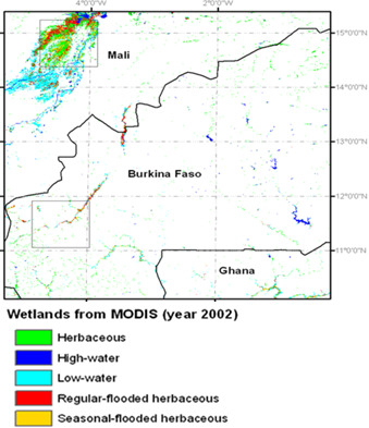
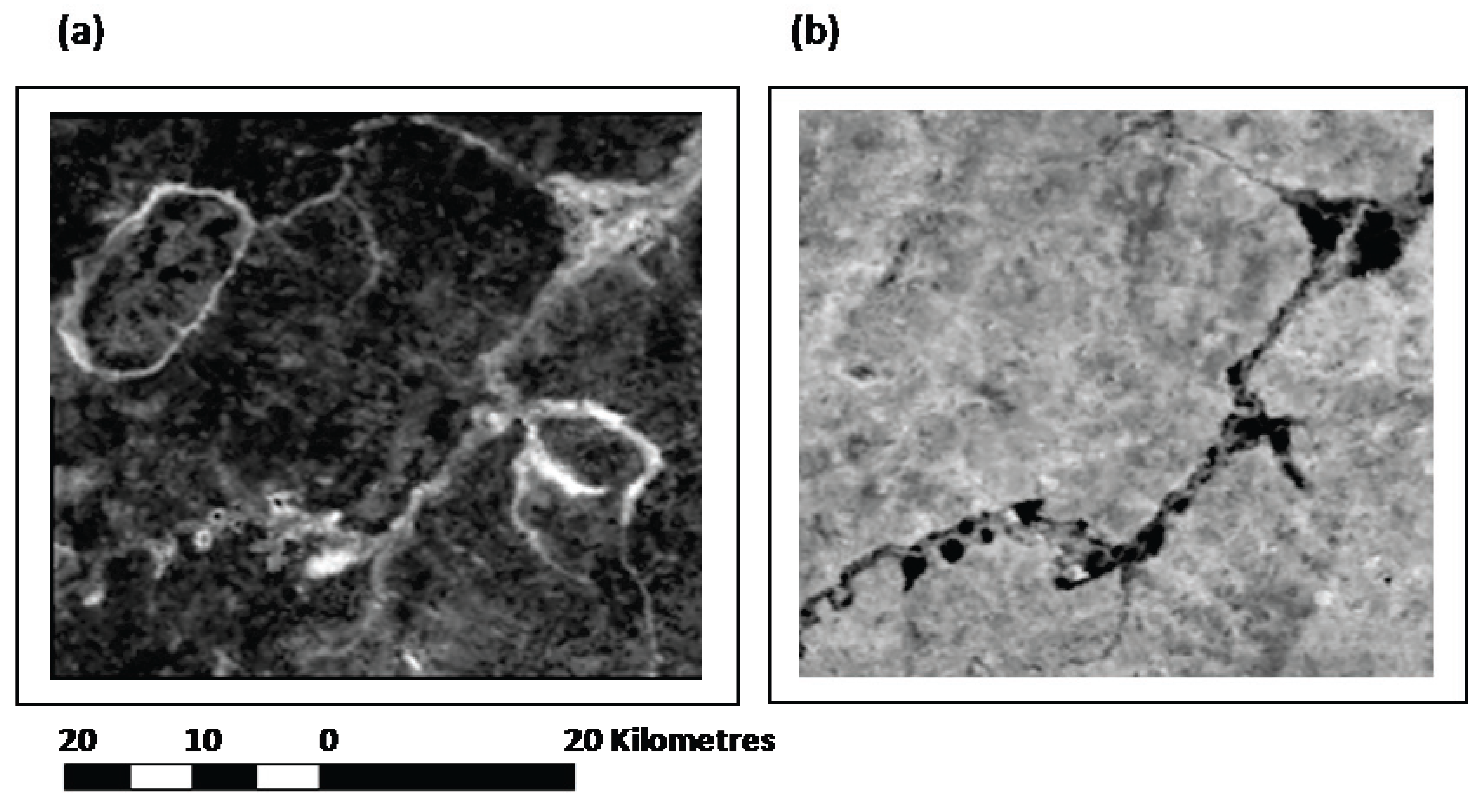
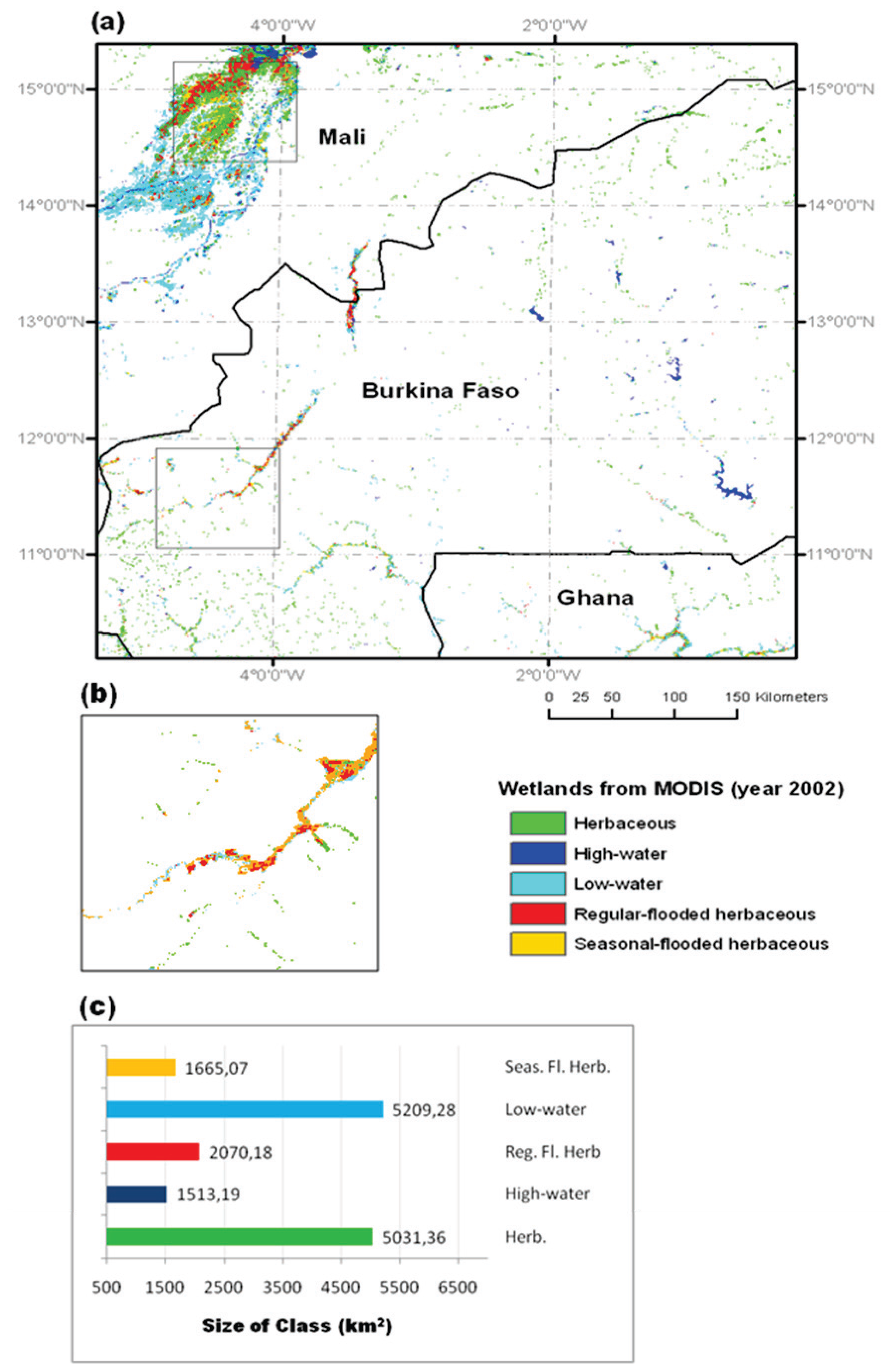
4.1 Spatial Patterns of Wetland Types

Figure 3a below shows the spatial distribution of the five classes for the whole study area, and zoomed in for the La Mare Hippotames site in western Burkina Faso in Figure 3b. The bar plot in Figure 3c shows the class size in squared kilometers (km2). The class “Low-water wetland” exhibits the biggest class coverage with over 5,209 km2 (cyan in Figure 3). This class is dominantly found in the Niger Delta, and from visual inspection in the Landsat data largely also includes rice paddy fields. The classes “Low-water wetland” and “High water wetland” are from their morphological character similar; both classes exhibit flooding in the wet season with none to low aquatic vegetation abundances (Table 1). As the NIR reflectance has proven sensitivity to the occurrence of water and wet soil (sludge) areas due to regular flooding [30], these two classes may include areas of wet soils or sludge areas that are regularly inundated. The class “Herbaceous wetland” is second in size (5,031 km2); this class often shows a distinct linear pattern within streamline areas especially in the south of the study area and may thus also include a woody life form component. However, since 89% of all wetland classes that are dominated by ‘herbaceous life form’ were found to be associated with the landform ‘pit’ or ‘pit and streamlines’, the assumption can be made that “Gallery Forests” within streamline areas were successfully masked. We used the topographic feature masking to exclude the class “Gallery Forests” from the final map product.
The classes “Regular flooded herbaceous wetland” and “Seasonal flooded herbaceous wetland”, show a linear pattern along the river channel that runs along the La Mare Hippotames site, as visible in Figure 3b. The distinct linear pattern and occurrence of ‘frequently flooded’ water pools alongside the river are due to regular flooding from the nearby river, and represent typical spatial patterns attributed to many wetland systems in West Africa [52]. Both of these classes also have the similar ‘greening’ and flooding behavior in the MODIS (Table 1). As such the two classes are rather ‘fuzzy’, pertaining to their flooding regime and abundance of vegetation, and thus they may include regularly flooded and/or seasonally flooded wetland (sub-) types with variable types of aquatic to semi-aquatic vegetation groupings.
The aerial extend of all wetland classes mapped within this sample area make up 4.3% of the total study area. For West Africa, we found an estimation of between 1.25 and 5.25% of the total land mass being wetland, excluding rivers which make up 2.25% of the land [53]. The national land cover data set for Burkina Faso, which is based on Landsat and field surveys from the years 2000–2002 and derived by the Institute de Geographie du Burkina-IGB [54,55], shows a wetland extend of 0.84%, compared to an estimate of 0.68% aerial coverage attained in this study for Burkina Faso. The IGB database, however, uses a different class coding thus a thematic comparison would not be valid. However since there is an overlap in the time periods, i.e., their data as well as our data sets are based on imagery from 2002, this is probably the best per country cross reference, considering only the generic class ‘wetlands’. A comparison to the 300-meter GLOBCOVER global land cover data base from the calendar year 2005 [56], which includes up to seven wetland categories within the regional land cover product, shows that there is little thematic and spatial overlap. In GLOBCOVER, the La Mare Hippotames site is largely mapped as “Closed to open shrubland” and “Mosaic Forest-Shrubland/Grassland”, whilst the Niger Delta site is mapped as “Closed to open vegetation regularly flooded”.
Figure 3. (a). Mapped wetlands over the whole study region. Solid line grey squares show the Landsat reference site locations. (b). zoomed map for the RAMSAR site La Mare Hippotames. (c). Bar chart showing the size of each of the five wetland classes in km2.
Remotesensing 02 01751 g003

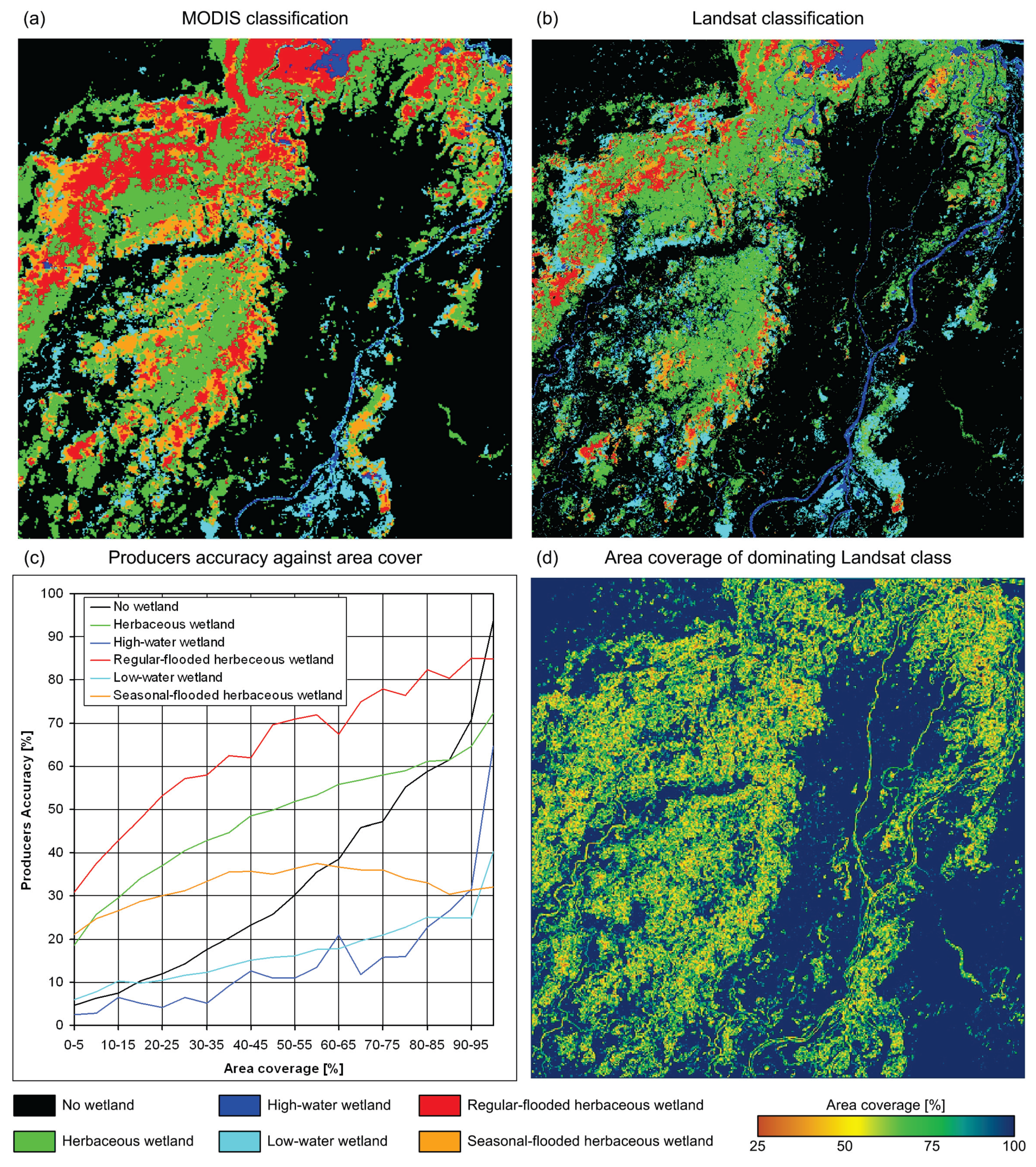
4.2. Accuracy Assessment Results

The classified result of the Landsat data is depicted in Figure 4b, here showing the Niger Delta site as an example. For moderate resolution imagery, such as MODIS, the use of pixel-based methods is problematic [32], due to the large spatial variability and ultimately the mapping of mixed pixels that is mixed classes [30,57]. Therefore, we accounted for the area-proportion of each class in the respective MODIS cell and also represented these proportions in the error matrix. Without resampling Landsat to the MODIS resolution, this approach incorporates the spatial detail of the Landsat data into the assessment.
The “Wetland”/“No wetland” separation for both sites can be considered ‘high’. The overall agreement (Kappa coefficient) was 84.2% (0.67) and 97.9% (0.59) for the inland Niger Delta and the La Mare Hippotames site, respectively. The high difference between overall accuracy and Kappa coefficient for La Mare Hippotames is due to the high number of “no wetland” pixels in the analysis. The accuracies herein (for all wetlands) compare well to mapping accuracies attained in Landsat data based studies elsewhere [10,58,59].
A detailed assessment including all wetland classes was conducted for the inland Niger Delta, for which the overall accuracy reached 66.6% with a KHAT of 0.46. The error matrix (Table 2) depicts high accuracies for classes “No wetland” and “Herbaceous wetland”. “High-water wetland” and “Regular-flooded herbaceous wetland” yielded high users respective producer accuracies. Due to low inundation levels in the class “Low-water wetland”, this class is primarily confused with “no wetland” as well as other classes that exhibit low inundation levels. Similarly “Seasonal-flooded herbaceous wetland” shows confusions with thematically related classes.
Table 2. Error matrix for the inland Niger Delta site showing all five wetland classes mapped from MODIS and reference classes from Landsat. Cell values indicate the area-agreement of Landsat and MODIS in km2. The users and producers accuracies are shown for all classes.
MODISLandsatUsers
012345
0No wetland4,712.971.746.11.6223.710.893.0
1Herbaceous wetland549.7867.79.884.6152.5125.948.5
2High-water wetland19.21.762.50.816.91.061.2
3Regular-flooded herb. wetland32.7352.127.3218.066.0209.524.1
4Low-water wetland285.316.045.80.9171.16.832.5
5Seasonal-flooded herb. wetland224.6199.817.721.9276.4169.918.7
Producers80.957.529.966.518.932.4
Figure 4 depicts some interesting patterns when assessing the MODIS classification with high-spatial resolution Landsat data (resolution ratio 7.7). Figure 4d shows the highest area proportion of a Landsat class within a MODIS cell. Although there are values close to or equal to 100% due to homogeneous areas in the Landsat map, many areas depict intermediate to low area proportions for mixed pixels when comparing Landsat to MODIS. Therefore, it is clear that spatially disperse classes with small patches such as “Low-water wetland” and “Seasonal-flooded herbaceous wetland” will yield low accuracies for less homogeneous pixels. The same accounts for linear features of “High-water wetland” which were detected in Landsat but are beyond the resolution of MODIS. Figure 4c illuminates the impact of area coverage, plotting the producers’ accuracies against area coverage in the Landsat data. The plot shows the good agreement for “Herbaceous wetland” and “Regular-flooded herbaceous wetland”, which are both spatially overestimated in the MODIS map. The concave form of “No wetland” indicates an underestimation for mixed pixels but homogeneous areas were classified very well. A similar trend is depicted for “High-water wetland” with accuracies below 30% even for 95% area cover but nearly 65% for 95–100% cover. This class maps open water such as rivers and streams in Landsat, which are often beyond the MODIS resolution. However the lake in the northern section makes a homogeneous area and was identified well in both, Landsat and MODIS.
Figure 4. (a). Image classification result from the MODIS data. (b). Image classification result from the Landsat data. (c). Producers accuracies as a function of area-coverage in 5% intervals (d). The area-coverage of the dominating class.
Remotesensing 02 01751 g004
In general, none of the five wetland classes shows high accuracies. Reasons for inaccuracies, apart from the inherent pixel variability and mapping errors, could be the high water and vegetation dynamics within wetlands that make these features challenging to assess even when high resolution data sets are used [12,18]. Especially in West Africa, wetlands may exhibit near to weekly alterations in water and vegetation compositions, largely due to wind, water table and water flow dynamics. Moreover they are highly heterogeneous in terms of their aquatic vegetation compositions, being mixtures of helophytes and hydrophytes [11]. In many ‘global’ land cover data sets (i.e., GLOBCOVER), the accuracy assessment of wetland classes is limited only to a few wetland classes [60], largely due to the reasons described and low amount of reference samples available. The use of finer per pixel inundation length from high to moderate resolution time-series data paired with in situ reference data on wetland morphology and ecology would be bases for improved time-related and mixed wetland class coding with higher class accuracies.

5. Conclusions

This study demonstrates the use and possibility of effectively mapping wetland classes based on seasonal ‘wetland behavior’ pertaining to chlorophyll activity (MODIS VI) and inundations in the wet season (MODIS NIR), using cost-free 250 m MODIS and 90 m SRTM data. Given that the general discrimination for “No wetland”/“Wetland” are very good at both reference sites, we propagate that the method used herein is suitable to wide area basic delineation of wetlands in these semi arid savannas.
Since we adhered to pre-processing routines, used a index function based on seasonal wetland behavior and the comparison to global land cover products show that we were able to discern more wetland classes whilst we showed that a generic comparison to local scale mapping results is possible (the IGB data set), we deem that the approach described herein is spatially interoperable and timely repeatable. Interoperability is further enhanced by the accuracy assessment as a function of area-coverage (Figure 4) that provides important information of how a class performs in accuracy assessment. If scaling effects in the classes are known, they can be implicated for wider area mapping. Due to the inherent challenges in mapping wetlands and limited reference data availability, especially in West Africa, we consider our five class result to be the most detailed wide area wetland data set available for West Africa.
The lower accuracies for each of the classes demonstrate the need for earth observation methods to not only base their assessments on satellite observations, but to also utilize linkages to other higher resolution and in situ point data sets.

Acknowledgements

We thank the German Ministry for Education and Research (BMBF) for funding this research activity, which was part of the BMBF funded BIOTA and the GLOWA Volta projects in West Africa. We would also like to thank the reviewers and colleagues at the Remote Sensing Department of the University of Wuerzburg for their useful comments and suggestions.

References

  1. Cowardin, L.M.; Carter, V.; Golet, F.; Laroe, E.T. Classification of Wetlands and Deepwater Habitats of the United States; US National Oceanographic and Atmospheric Administration Office of Coastal Zone Management: Washington, DC, USA, 1979.
  2. Thomas, K.L.; Benstead, J.; Davies, K.L.; Lloyd, D. Role of wetland plants in the diurnal control of CH4 and CO2 fluxes in peat. Soil Biol. Biochem. 1996, 28, 17–23. [Google Scholar] [CrossRef]
  3. Finlayson, M.; Moser, M. Wetlands; International Waterfowl and Wetlands Research Bureau: New York, NY, USA, 1991. [Google Scholar]
  4. Hails, A.J. Wetlands, Biodiversity, and the Ramsar Convention; Ramsar Convention Bureau: Gland, Switzerland, 1997. [Google Scholar]
  5. Mitsch, W.J.; Gosselink, J.G. Wetlands, 3rd ed.; John Wiley and Sons: New York, NY, USA, 1997. [Google Scholar]
  6. Lewis, W.M. Wetland: Characteristics and Boundaries, 1st ed.; National Academy Press: Washington, DC, USA, 1995. [Google Scholar]
  7. Tiner, R.W. Wetland Indicators: A Guide to Wetlands Identification, Delineation, Classification, and Mapping, 1st ed.; CRC Press: Boca Raton, FL, USA, 1999. [Google Scholar]
  8. Weller, D.E.; Snyder, M.N.; Whigham, D.F.; Jacobs, A.D.; Jordan, T.E. Landscape indicators of wetland condition in the Nanticoke River Watershed, Maryland and Delaware, USA. Wetlands 2007, 27, 498–514. [Google Scholar] [CrossRef]
  9. Kansiime, F.; Saunders, M.J.; Loiselle, S.A. Functioning and dynamics of wetland vegetation of Lake Victoria: An overview. Wetlands Ecol. Manag. 2007, 15, 433–451. [Google Scholar] [CrossRef]
  10. Townsend, P.T.; Walsh, S.J. Remote sensing of forested wetlands: Application of multitemporal and multispectral satellite imagery to determine plant community composition and structure in Southeastern USA. Plant Ecology 2001, 157, 129–149. [Google Scholar] [CrossRef]
  11. Wittig, R. The Syntaxonomy of the Aquatic Vegetation of Burkina Faso, 1st ed.; Wittig, R., Guinko, S., Eds.; Verlag Natur und Wissenschaft: Solingen, Germany, 2005; Volume 9. [Google Scholar]
  12. Jones, K.; Lanthier, Y.; van der Voet, P.; van Valkengoed, E.; Taylor, D.; Fernandez-Prieto, D. Monitoring and assessment of wetlands using Earth Observation: The GlobWetland project. J. Environ. Manag. 2009, 90, 2154–2169. [Google Scholar] [CrossRef] [PubMed]
  13. Finlayson, C.M. The challenge of integrating wetland inventory, assessment and monitoring Aquatic Conservation. Marine Freshwater Ecosyst. 2003, 13, 281–286. [Google Scholar] [CrossRef]
  14. Di Gregorio, A.; Jansen, L.J.M. Land Cover Classification System (LCCS). Classification Concepts and User Manual; Food and Agricultural Organization (FAO) Environment and Natural Resources Services: Rome, Italy, 2005. [Google Scholar]
  15. Amezaga, J.M.; Santamaria, L.; Green, A.J. Biotic wetland connectivity—Supporting a new approach for wetland policy. Acta Oecol. 2002, 23, 213–222. [Google Scholar] [CrossRef]
  16. Weber, T. Landscape ecological assessment of the Chesapeake Bay watershed. Environ. Monitor. Assessment 2004, 94, 39–53. [Google Scholar] [CrossRef]
  17. Tiner, R.W. Estimated extend of geographically isolated wetlands in selected areas of the United States. Wetlands 2003, 23, 636–652. [Google Scholar] [CrossRef]
  18. Nielsen, E.M.; Prince, S.D.; Koeln, G.T. Wetland change mapping for the U.S. mid-Atlantic region using an outlier detection technique. Remote Sens. Environ. 2008, 112, 4061–4074. [Google Scholar] [CrossRef]
  19. IUCN. Reducing West Africa’s Vulnerability to Climate Change Impacts on Water Resources, Wetlands and Desertification: Elements for a Regional Strategy for Preparedness and Adaptation, 1st ed.; Niasse, M., Afouda, A., Amani, A., Eds.; IUCN: Gland, Switzerland, 2004. [Google Scholar]
  20. Saunders, M.J.; Jones, M.B.; Kansiime, F. Carbon and water cycles in tropical papyrus wetlands. Wetlands Ecol. Manag. 2007, 15, 489–498. [Google Scholar] [CrossRef]
  21. Muchoney, D.M. Earth observations for terrestrial biodiversity and ecosystems. Remote Sens. Environ. 2008, 112, 190–191. [Google Scholar] [CrossRef]
  22. MacKay, H.; Finlayson, C.M.; Fernandez-Prieto, D.; Davidson, N.; Pritchard, D.; Rebelo, L.M. The role of Earth Observation (EO) technologies in supporting implementation of the Ramsar Convention on Wetlands. J. Environ. Manag. 2009, 90, 2234–2242. [Google Scholar] [CrossRef] [PubMed]
  23. Peter, N. The use of remote sensing to support the application of multilateral, environmental agreements. Space Policy 2004, 20, 189–195. [Google Scholar] [CrossRef]
  24. MedWet. Inventory, Assessment and Monitoring of Mediterranean Wetlands: Mapping Wetlands Using Earth Observation Techniques, 1st ed.; Fitoka, E., Keramitsoglou, F., Eds.; MedWet: Thessaloniki, Greece, 2008. [Google Scholar]
  25. Rebelo, L.M.; Finlayson, C.M.; Nagabhatla, N. Remote sensing and GIS for wetland inventory, mapping and change analysis. J. Environ. Manag. 2009, 90, 2144–2153. [Google Scholar] [CrossRef] [PubMed]
  26. Barnes, W.L.; Pagano, T.S.; Salomonson, V.V. Prelaunch characteristics of the Moderate Resolution Imaging Spectroradiometer (MODIS) on EOS-AMI. IEEE Trans. Geosci. Remote Sens. 1998, 36, 1088–1100. [Google Scholar] [CrossRef]
  27. Vekerdy, Z.; Gross, D. Monitoring of riverine wetland dynamics with MODIS images. In Proceedings of the EGS-AGU-EUG Joint Assembly, Nice, France, April 2003.
  28. Colditz, R.; Keil, M.; Strohbach, B.; Gessner, U.; Schmidt, M.; Dech, S. Vegetation structure mapping with remote sensing time series: Capabilities and improvements. In Proceedings of the 32nd International Symposium on Remote Sensing of Environment, San Jose, Costa Rica, June 2007.
  29. Conrad, C.; Dech, S.; Hafeez, M.; Lamers, J.; Martius, C.; Strunz, G. Mapping and assessing water use in a Central Asian irrigation system by utilizing MODIS remote sensing products. Irrig. Drain. Syst. 2005, 21, 197–218. [Google Scholar] [CrossRef]
  30. Xiao, X.; Boles, S.; Liu, J.; Zhuang, D.; Frolking, S.; Li, C.; Salas, W.; Moore, B. Mapping paddy rice agriculture in southern China using multi-temporal MODIS images. Remote Sens. Environ. 2005, 95, 480–492. [Google Scholar] [CrossRef]
  31. Thenkabail, P.; Schull, M.; Turral, H. Ganges and Indus river basin land/use/land cover (LULC) and irrigation area mapping using continuous streams of MODIS data. Remote Sens. Environ. 2004, 95, 317–341. [Google Scholar] [CrossRef]
  32. Knight, J.F.; Lunetta, R.L.; Ediriwickrema, J.; Khorram, S. Regional scale land-cover characterization using MODIS-NDVI 250m Multi-Temporal Imagery: A phenology based approach. GISci. Remote Sens. 2006, 43, 2–23. [Google Scholar] [CrossRef]
  33. Harvey, K.R.; Hill, G. Vegetation mapping of a tropical freshwater swamp in the Northern Territory, Australia: A comparison of aerial photography, Landsat TM and SPOT satellite imagery. Int. J. Remote Sens. 2001, 22, 2911–2925. [Google Scholar] [CrossRef]
  34. Bock, M.; Xofis, P.; Mitchley, J. Object-oriented methods for habitat mapping at multiple scales—Case studies from Northern Germany and Wye Downs. J. Nature Conserv. 2005, 13, 75–89. [Google Scholar] [CrossRef]
  35. Baker, C.; Lawrence, R.; Montagne, C.; Patten, D. Mapping wetlands and riparian areas using Landsat ETM+ imagery and decision-tree-based models. Wetlands 2006, 26, 465–74. [Google Scholar] [CrossRef]
  36. Jensen, J.R.; Narumalani, S.; Weatherbee, O.; Mackey, H.E. Measurement of seasonal and yearly cattail and waterlily changes using multidate SPOT panchromatic data. Photogramm. Eng. Remote Sens. 1993, 59, 519–525. [Google Scholar]
  37. Sersland, C.A.; Johnston, C.; Bonde, J. Assessing wet land vegetation with GPS-linked, color video image mosaics. In Proceedings of the ASPRS 15th Biennial Workshop on Vidcography and Color Photography in Resource Assessment, Terre Haute, IN, USA; 1995. [Google Scholar]
  38. Wolter, P.T.; Johnston, C.A.; Niemi, G.J. Mapping submerged aquatic vegetation in the U.S. Great Lakes using Quickbird satellite data. Int. J. Remote Sens. 2005, 26, 55–74. [Google Scholar] [CrossRef]
  39. Hubert-Moy, L.; Clément, B.; Lennon, M.; Houet, T.; Lefeuvre, E. Study of wetlands using CASI hyperspectral images: Application to the valley floors of the Armorican Massif. Photo-Interprétation 2003, 39, 33–43. [Google Scholar]
  40. Dapaah-Siakwan, S.; Gyau-Boakye, P. Hydrogeologic framework and borehole yields in Ghana. Hydrogeol. J. 2000, 8, 405–416. [Google Scholar] [CrossRef]
  41. Hayward, D.F.; Oguntoyinbo, J.S. The Climatology of West Africa, 1st ed.; Barnes and Noble Books: Totowa, NJ, USA, 1987. [Google Scholar]
  42. Driessen, P.; Deckers, J.; Spaargaren, O. Lectures Notes on the Major Soils of the World; FAO World Soil Resources Report-94; Food and Agriculture Organization of the United Nations: Rome, Italy, 2001. [Google Scholar]
  43. Justice, C.O.; Townshend, J.R.G.; Vermote, E.F.; Masouka, E.; Wolfe, R.E.; Saleous, S.; Roy, D.P.; Morisette, J.T. An overview of MODIS Land data processing and product status. Remote Sens. Environ. 2002, 83, 3–15. [Google Scholar] [CrossRef]
  44. Huete, A.; Didan, K.; Miura, T.; Rodriguez, E.; Gao, X.; Ferreira, L. Overview of the radiometric and biophysical performance of the MODIS vegetation indices. Remote Sens. Environ. 2002, 83, 195–213. [Google Scholar] [CrossRef]
  45. Colditz, R.; Conrad, C.; Wehrmann, T.; Schmidt, M.; Dech, S. TiSeG: Flexible software tool for time-series generation of MODIS data utilizing the quality assessment science data set. IEEE Trans. Geosci. Remote Sens. 2008, 46, 3296–3308. [Google Scholar] [CrossRef]
  46. Fontes, J.; Guinko, S. Carte de végétation et de l'occupation du sol du Burkina Faso; Projet Campus, UPS, ICIV: Toulouse, France, 1995. [Google Scholar]
  47. Jensen, S.K.; Domingue, J.O. Extraction of topographic structure from digital elevation data for geographic information system analysis. Photogramm. Eng. Remote Sens. 1988, 54, 1593–1600. [Google Scholar]
  48. O’Callaghan, J.F.; Mark, D.M. The extraction of drainage networks from digital elevation data. Comput. Vis. Graph. Image Process. 1984, 28, 328–344. [Google Scholar]
  49. Rosenquist, A.; Forsberg, B.R.; Pimentel, T.; Rauste, Y.A.; Richey, J.E. The use of spaceborne radar data to model inundation patterns and trace gas emissions in the central Amazon floodplain. Int. J. Remote Sens. 2002, 23, 1303–1328. [Google Scholar] [CrossRef]
  50. Tou, J.T.; Gonzalez, RC. Pattern Recognition Principles, 1st ed.; Addison-Wesley: Reading, MA, USA, 1974. [Google Scholar]
  51. Reinelt, L.; Taylor, B.; Horner, R.R. Morphology and hydrology. In Wetlands and Urbanization-Implications for the Future, 1st ed.; Azous, A., Horner, R., Eds.; Lewis Publishers: Boca Raton, FL, USA, 2001; Volume 1, pp. 31–36. [Google Scholar]
  52. Nyarko, B.K. Floodplain Wetland-River Flow Synergy in the White Volta Basin of Ghana. Ph.D. Thesis, Rheinische Friedrich Wilhelms University, Bonn, Germany, 2007. [Google Scholar]
  53. Tappan, G.G.; Sall, M.; Wood, E.C.; Cushing, M. Ecoregions and land cover trends in Senegal. J. Arid Environ. 2003, 59, 427–462. [Google Scholar] [CrossRef]
  54. IGB. Guide Technique de la Nomenclature BDOT Burkina Faso; IGN-FI: Ouagadougou, Burkina Faso, 2005. [Google Scholar]
  55. Costantini, C.; Ayala, D.; Guelbeogo, W.M. Living at the edge: Biogeographic patterns of habitat segregation conform to speciation by niche expansion in Anopheles gambiae. BMC Ecol. 2009, 9, 2–28. [Google Scholar]
  56. Defourny, P.; Bicheron, P.; Brockman, C.; Bontemps, S.; van Bogaert, E.; Vancutsem, C. The first 300 m global land cover map for 2005 using ENVISAT MERIS time series: A product of the GlobCover system. In Proceedings of the 33th International Symposium of Remote Sensing of Environment, Stresa, Italy, May 2009.
  57. Lunetta, R.S.; Alvarez, R.; Edmonds, C.M.; Lyon, J.G.; Elvidge, C.D.; Boniface, R.; Garcia, C. NALC/Mexico land-cover mapping results: implications for assessing landscape condition. Int. J. Remote Sens. 2002, 23, 3129–3148. [Google Scholar] [CrossRef]
  58. Kovacs, J.M.; Wang, J.; Blanca-Correa, M. Mapping disturbances in a mangrove forest using multidate Landsat TM imagery. Environ. Manag. 2001, 27, 763–776. [Google Scholar] [CrossRef]
  59. Sader, S.A.; Ahl, D.; Liou, W.S. Accuracy of Landsat TM and GIS rule-based methods for forest wetland classification in Maine. Remote Sens. Environ. 1995, 53, 133–144. [Google Scholar] [CrossRef]
  60. Bicheron, P.; Defourny, P.; Schouten, C.B.L.; Vancutsem, C.; Huc, M.; Bontemps, S.; Leroy, M.; Achard, F.; Herold, M.; Ranera, F.; Arino, O. GLOBCOVER—Products description and validation report, medias France technical documants. Available online: http://postel.mediasfrance.org/en/ DOWNLOAD/Documents/ (accessed on 10 March 2010).

