A New Approach to Change Vector Analysis Using Distance and Similarity Measures

Abstract

The need to monitor the Earth’s surface over a range of spatial and temporal scales is fundamental in ecosystems planning and management. Change-Vector Analysis (CVA) is a bi-temporal method of change detection that considers the magnitude and direction of change vector. However, many multispectral applications do not make use of the direction component. The procedure most used to calculate the direction component using multiband data is the direction cosine, but the number of output direction cosine images is equal to the number of original bands and has a complex interpretation. This paper proposes a new approach to calculate the spectral direction of change, using the Spectral Angle Mapper and Spectral Correlation Mapper spectral-similarity measures. The chief advantage of this approach is that it generates a single image of change information insensitive to illumination variation. In this paper the magnitude component of the spectral similarity was calculated in two ways: as the standard Euclidean distance and as the Mahalanobis distance. In this test the best magnitude measure was the Euclidean distance and the best similarity measure was Spectral Angle Mapper. The results show that the distance and similarity measures are complementary and need to be applied together.

1. Introduction

Change-Vector Analysis (CVA) [1] is a bi-temporal method that was originally designed for only two spectral dimensions (2-D CVA): Brightness (an indicator of overall reflectance) and Greenness (an indicator of vegetation), both from the Tasseled Cap transform [2]. The CVA produced as output two change components: magnitude and direction.

CVA application for >2 spectral bands (3-D CVA or higher) uses the same calculation of the magnitude; however the calculation of the direction can be done with several different methods. In many cases the direction component is disregarded entirely [3]. Two approaches have been proposed for calculating the direction component in 3-D CVA: sector-coding [4] and calculating vector direction cosines [5]. The sector-coding scheme defines nominal categories for change direction. However, this procedure tends to be complex for >3 spectral bands and under utilizes the data variance. In contrast, the direction cosines procedure offers a practical approach that can be extended to n-dimensional space (n-D CVA) [6,7].

The mathematical framework of the n-D CVA calculation is presented below. If $X^{t_1}=\{x_1^{t_t},x_2^{t_1},\dots ,x_N^{t_1}\}$ and $X^{t_2}=\{x_1^{t_2},x_2^{t_2},\dots ,x_N^{t_2}\}$ are the sets of N spectral bands of images acquired at time t₁ and t₂, respectively, the angle between the vector and each axis (θ₁, θ₂, θ₃,…θ_N) can be expressed by the arccosine function:

$${\theta }_i={\cos }^{-1}\left(\frac{X_i^{t_1}-X_i^{t_2}}{ED}\right) i= 1\dots N$$

(1)

where ED is the Euclidian distance between two temporal spectra ($X^{t_1}$ and $X^{t_2}$), expressed as the square root of the band-wise sum of the squares of the differences:

$$ED=\sqrt{{{\displaystyle \sum }}_{i=1}^N{\left(X_i^{t_1}-X_i^{t_2}\right)}^2}$$

(2)

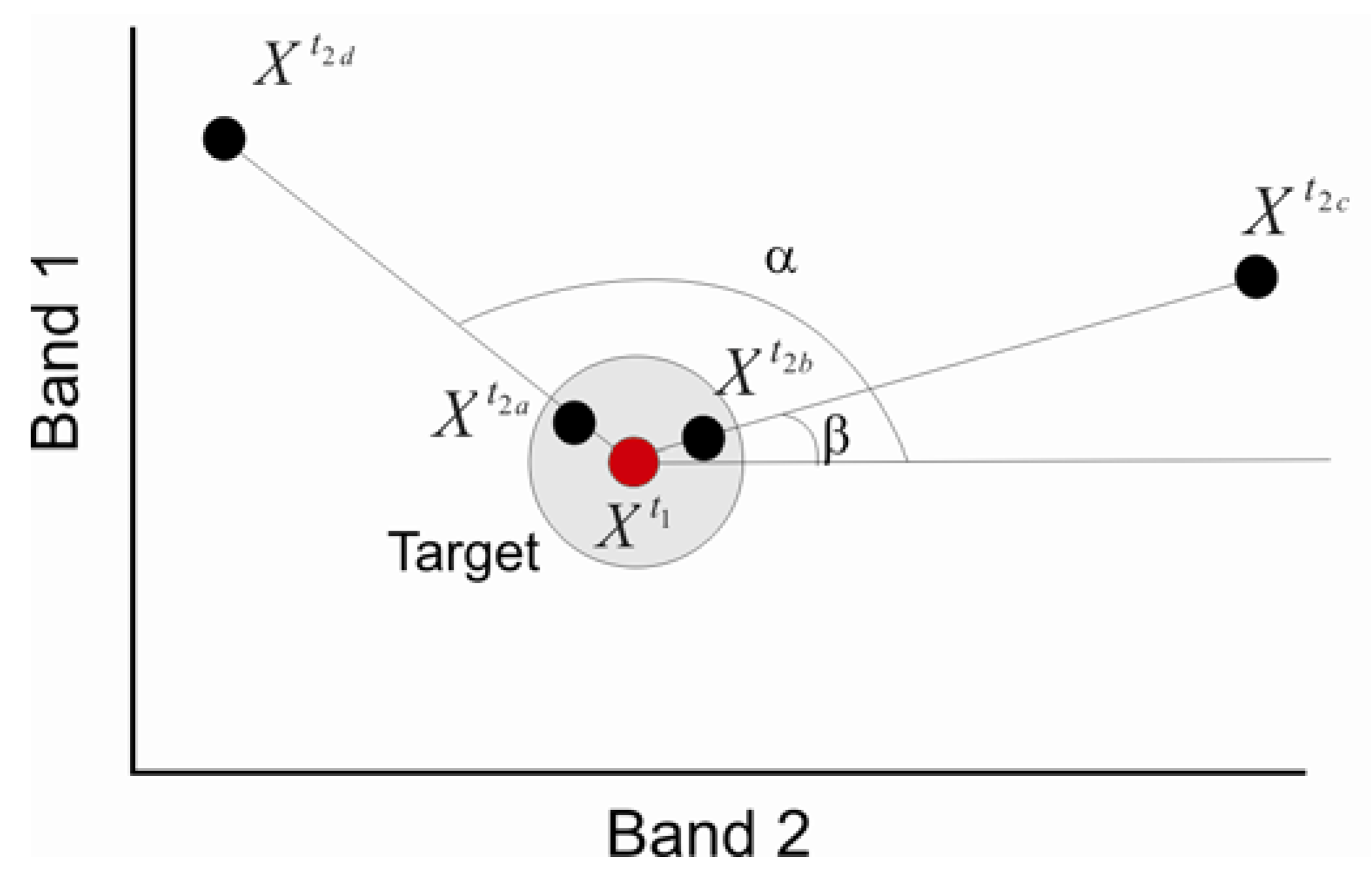
However, the number of the direction cosines equals the number of bands (axes), which complicates the analysis and change identification. Moreover, the direction cosine method generates images and information that are difficult to understand in terms of surface components. No-change pixels rarely have exactly the same values. These pixels cluster about some centroid in a spherical distribution, such that the direction-of-change vectors can easily have high variable angles, and these are manifested as extreme variability in the direction cosine images.

Figure 1 illustrates the difficulty of interpreting direction cosine. Although points $X^{t_1}$, $X^{t_{2a}}$, and $X^{t_{2b}}$ all represent “real” measurements, including errors, of a target (point $X^{t_1}$ in Figure 1), their vector angles are very different (α and β). Furthermore, despite no meaningful change between $X^{t_1}$ and $X^{t_{2a}}$, the vector angle between $X^{t_1}$ and $X^{t_{2a}}$ is the same as between $X^{t_1}$ and $X^{t_{2d}}$, for which change is significant. These cases cannot be told apart with the information available, nor can ($X^{t_1}$ and $X^{t_{2b}}$) and ($X^{t_1}$ and $X^{t_{2c}}$).

Figure 1. Two-dimensional space having change vectors with the same angles α $X^{t_{1 }}$ − $X^{t_{2a}}$ and $X^{t_1}$ − $X^{t_{2d}}$) and β ($X^{t_1}$ − $X^{t_{2b}}$ and $X^{t_1}$ − $X^{t_{2c}}$). Two of the vectors represent no-change ($X^{t_1}$ − $X^{t_{2a}}$ and $X^{t_1}$ − $X^{t_{2b}}$) and two represent change ($X^{t_1}$ − $X^{t_{2c}}$ and $X^{t_1}$ − $X^{t_{2d}}$). The gray disk is a standard deviation for the no-change vectors.

Figure 1. Two-dimensional space having change vectors with the same angles α $X^{t_{1 }}$ − $X^{t_{2a}}$ and $X^{t_1}$ − $X^{t_{2d}}$) and β ($X^{t_1}$ − $X^{t_{2b}}$ and $X^{t_1}$ − $X^{t_{2c}}$). Two of the vectors represent no-change ($X^{t_1}$ − $X^{t_{2a}}$ and $X^{t_1}$ − $X^{t_{2b}}$) and two represent change ($X^{t_1}$ − $X^{t_{2c}}$ and $X^{t_1}$ − $X^{t_{2d}}$). The gray disk is a standard deviation for the no-change vectors.

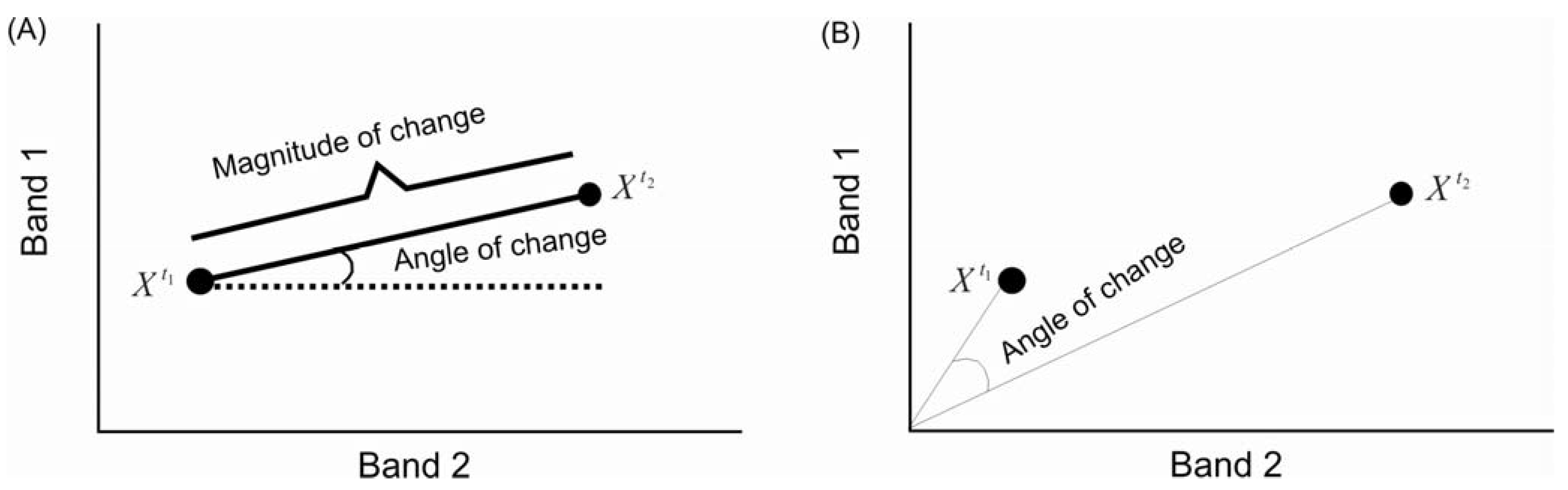
To avoid the above situation, this paper proposes to determine the direction of change from the angle between the two temporal vectors, instead of using the angle between the change vector and the axes of the Cartesian space used to describe the image vectors. Figure 2 shows conceptually the two approaches for angle-direction calculation in a bi-dimensional space. In our approach, two spectral vectors at different times are considered. Each temporal spectral vector is drawn from the origin through one of the data points. If two points are on the same vector, it indicates no change in spectral shape or contrast, just different degrees of shading. Thus, the origin of coordinates represents null reflectance, and shade decreases with distance away from the origin. It should be noted that this approach is insensitive to real change in the albedo of a surface component that mimics darkening due to an illumination variation.

Figure 2. Two concepts in calculating the change angle of a pixel for the first (t₁) and second (t₂) times: (a) magnitude and direction of change vector, relative to a projection of the x axis (dotted line), from Malila (1980); and (b) angle of change between spectral vectors for a pixel X at t₁ and t₂.

Figure 2. Two concepts in calculating the change angle of a pixel for the first (t₁) and second (t₂) times: (a) magnitude and direction of change vector, relative to a projection of the x axis (dotted line), from Malila (1980); and (b) angle of change between spectral vectors for a pixel X at t₁ and t₂.

In this study a new algorithm is formulated to calculate the direction of change in CVA using an adaptation of the Spectral Angle Mapper and the Spectral Correlation Mapper. Although Change-Vector Analysis (CVA) has often used the Euclidian distance in calculating the magnitude of change vector, the Mahalanobis distance has also been used [8,9]. Thus, we compare the use of the Mahalanobis and Euclidian distances to estimate the magnitude of change. All methods discussed were implemented in software developed in C++, available in a supplementary file.

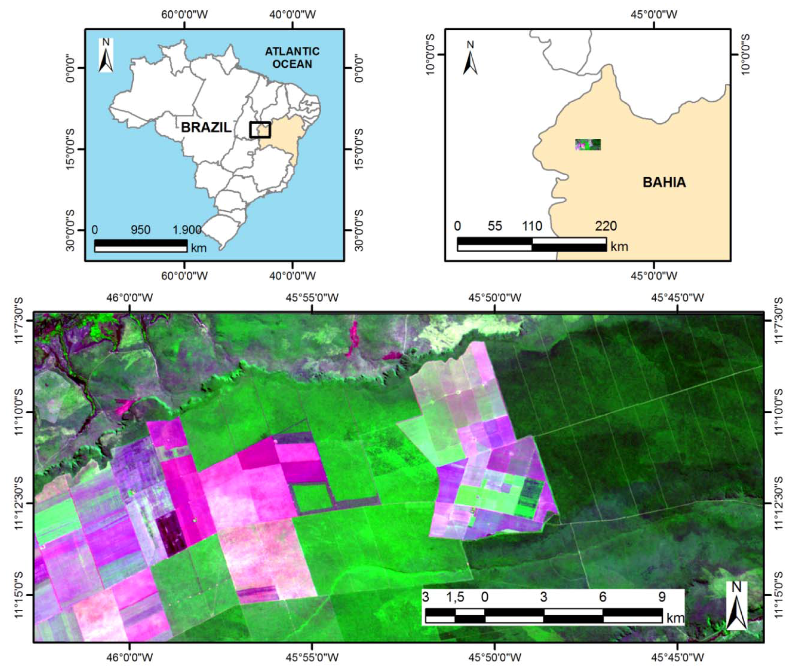
The proposed methods have been applied in the Cerrado region of Western Bahia state of Brazil, which since the 1980s has become the leading region of an expanding agricultural frontier in northeastern Brazil (Figure 3). Factors there attractive to farmers are the low cost of land, high insolation, flat topography, proximity to population centers in northeastern Brazil, government policy for land acquisition and low interest rates for the agricultural production [10,11]. The highest precipitation is 1,600 mm/yr, mostly in the rainy season from October to March. The lowest precipitation is in dry season from May to October. The different types of land use and the many changes over time make this area suitable for testing remote change-detection methods in a tropical environment.

Figure 3. Study area. Landsat TM (bands 3, 4, 5 as RGB) from 17 June 2006 (path 220, row 68).

Figure 3. Study area. Landsat TM (bands 3, 4, 5 as RGB) from 17 June 2006 (path 220, row 68).

2. Methods

2.1. Pre-Processing

An important factor in change detection is the choice of the temporal images to be analyzed. Preferably, images should be selected from the same sensor, acquired under similar illumination geometries, and in a similar environmental condition. Thus, images from the same time of year are often used in multi-temporal studies to minimize phenological effects and sun-terrain-sensor geometry. In the present paper are used Landsat TM (Thematic Mapper) images of the Cerrado acquired during the same months (20 June 1984 and 17 June 2006).

The two main requirements in pre-processing for bi-temporal change detection are precise registration of the images and radiometric and atmospheric calibration [12,13]. In this work the images were co-registered from ground control points identified in each image.

Misregistration compromises the accuracy of change detection. Images have to be superimposed within 0.2 pixel root mean squared error (RMS) to achieve an error of only 10% [14,15]. For this work the Landsat 5 TM images were co-registered (1984 and 2006) using ENVI software. In registration were selected 15 ground control points. A third-order polynomial function was applied in those coordinates which misregistrations could be identified, pixel by pixel, and corrected. The RMS value was <0.2 pixel.

For change detection, it is helpful to identify and remove changes caused by extraneous factors such as differences in atmospheric conditions, illumination and viewing angles, and sensor oscillation, in order to highlight only the spectral changes of interest. Thus, methods for a radiometric consistency among multi-temporal images are necessary for accurate landscape change detection. In previous studies, two levels of radiometric correction have been developed: absolute and relative.

In absolute radiometric correction, atmospheric radiative-transfer codes are used to obtain the reflectance at the Earth’s surface from the measured spectral radiances. The absolute methods correct for following factors: change in satellite sensor calibration over time, differences among in-band solar spectral irradiance, solar angle, variability in Earth-Sun distance, and atmospheric interferences.

In contrast, relative corrections normalize the digital counts to a common scale [16]. Thus, the radiometric properties of a subject image are adjusted to a reference image. This normalization has been developed considering mainly landscape elements for which reflectance values are nearly constant over time (these are called “pseudo-invariant features”, or PIFs), and linear regression over PIFs assuming that the pixels sampled in the same places at different times are linearly correlated [17,18,19]. In this paper a relative normalization was made from selected PIFs.

2.2. Change detection Using Spectral Measures

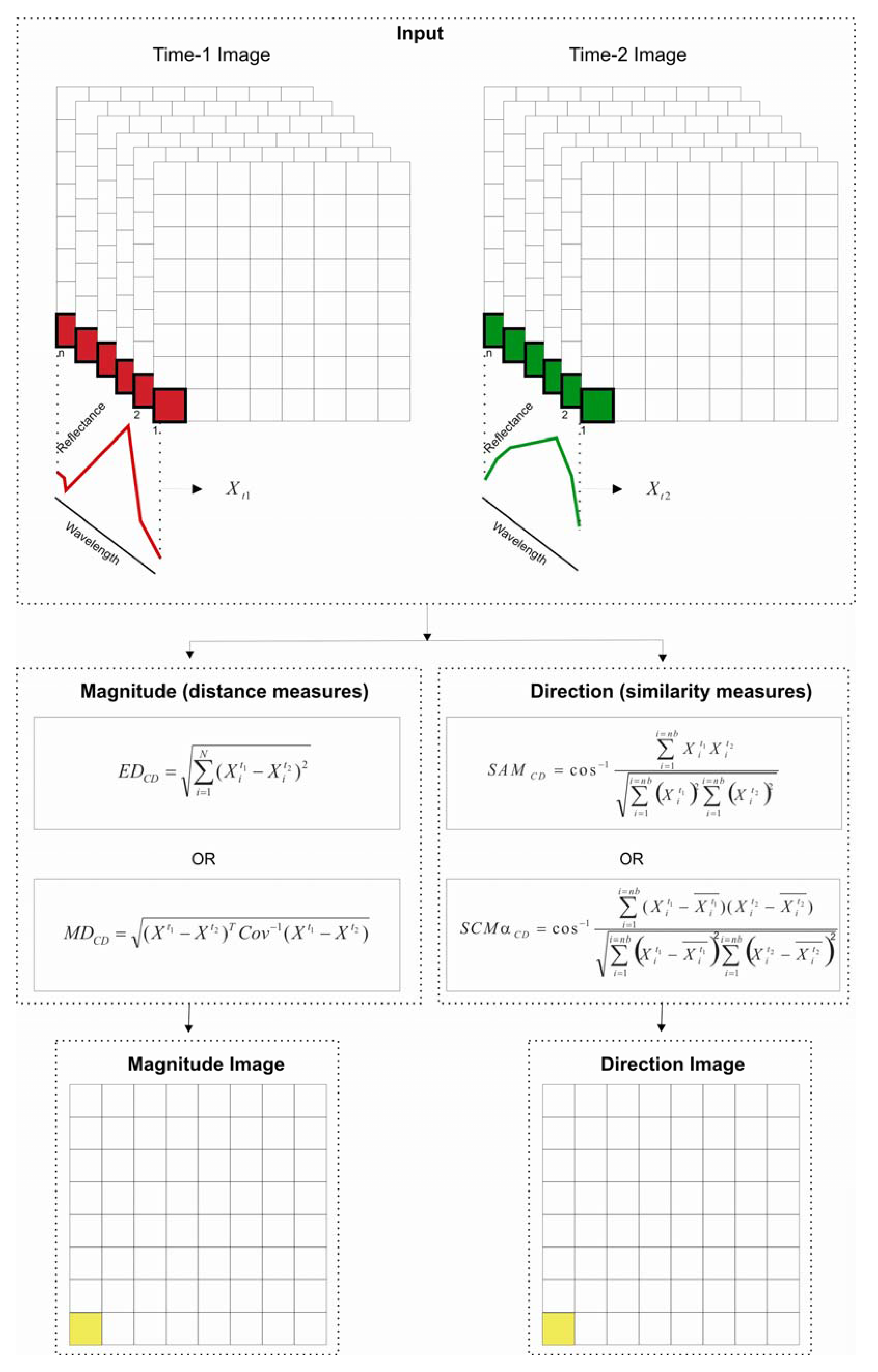
In this paper we estimate the magnitude of change by distance measures and the direction of change by similarity measures. The types of measures used to assess spectral distance and similarity are important topics in spectral classification theory. Spectral classifiers compare image spectra to a reference spectrum from spectral libraries or to spectral endmembers [20]. In this study the approach is to compare spectra measured at different times (Figure 4). Regardless of how the spectral relationships are defined, such analysis requires a suitable metric to capture the dependencies among variables. The target identification method adopted was based on the best optimum threshold. In the case of spectral classification, the best fit indicates the greatest possibility of a reference material in a given pixel; for change detection it indicates no spectral change in time.

Figure 4. Scheme for change detection using spectral measures.

Figure 4. Scheme for change detection using spectral measures.

However, many measures of spectral distance and similarity provide conflicting information about the target. This is because each measure has its own classification bias, which justifies the use of different measures in accordance with the situation and data type [20]. Thus, one important step is to discover the main relations of the temporal spectra to apply the best metric or a combination of metrics for a given situation.

2.3. Direction of Vector Change (Correlation Measures)

The main correlation measures that have been employed in spectral classification are cosine correlation in the Spectral Angle Mapper (SAM), and Pearson’s correlation coefficient in the Spectral Correlation Mapper (SCM). SAM is a common method of spectral classification [21] and is widely used in geological mapping [22,23] and space science [24]. In this work, the SAM expression is adapted to change detection (SAM_CD) considering the registered pixel X for the first (t₁) and second (t₂) times:

$$SA{M}_{CD}=\alpha = co{s}^{-1}\frac{{{\displaystyle \sum }}_{i=1}^{i=N}{X}_i^{t_1}{X}_i^{t_2}}{\sqrt{{{\displaystyle \sum }}_{i=1}^{i=N}{\left(X_i^{t_1}\right)}^2{{\displaystyle \sum }}_{i=1}^{i=N}{\left(X_i^{t_2}\right)}^2}}$$

(3)

where “α” is the angle expressed in radians (0–π). The variable “i” corresponds to the spectral band and ranges from 1 to the number of bands (N). Smaller angles represent closer matches and indicate increased similarity between the two temporal spectral vectors.

SAM normalizes for the influence of shading and accentuates the target spectral-shape characteristics. This attribute insensitivity to shade is important for change detection, because in temporal data it is common to have illumination variation and shadow. The degree of change in spectral shape is described by the increase of the angle between the two temporal vectors. Different than the direction cosine method, in our approach the angle-direction component is represented by a single image, not multiple images whose number depends on the number of bands used. This is because the direction cosine method generates only one vector that is projected onto all axes of data space, whereas in our approach only the single angle between two temporal spectral vectors in a n-dimensional space is calculated.

SAM is unable to detect negatively correlated data, and correlation is sensitive to offset factors. In order to correct these limitations, an SCM method adopts Pearson’s correlation [25]. The SCM for change detection (SCM_CD) applies the following expression to the pixel X at the two times t₁ and t₂:

$$SC{M}_{CD}=\frac{{{\displaystyle \sum }}_{i=1}^{i=N}\left(X_i^{t_1}-\overline{X^{t_1}}\right)\left(X_i^{t_2}-\overline{X^{t_2}}\right)}{\sqrt{{{\displaystyle \sum }}_{i=1}^{i=N}{\left(X_i^{t_1}-\overline{X^{t_1}}\right)}^2{{\displaystyle \sum }}_{i=1}^{i=N}{\left(X_i^{t_2}-\overline{X^{t_2}}\right)}^2}}$$

(4)

SCM_CD can also be expressed as an angle, applying the arc-cosine.

$$SCM{\alpha }_{CD}=\alpha =co{s}^{-1}\left(SC{M}_{CD}\right)$$

(5)

The SCM_CD value varies between 1 and −1, with 1 meaning that the two series are identical, 0 meaning they are completely uncorrelated, and −1 meaning they are perfect opposites. The major difference between the correlation methods is that SAM_CD uses integral values for $X^{t_1}$ and $X^{t_2}$, whereas SCM_CD uses centered data by means $\overline{X^{t_1}}$ and $\overline{X^{t_2}}$ respectively. Thus, the cosine correlation is equivalent to the uncentered version of Pearson’s correlation assuming that the mean of the population is zero.

This normalization makes SCM_CD better than SAM_CD for detecting spectral shapes, due to its invariance under linear transformation of the data. That is, if you change the spectra by a gain (multiplicative) factor or by a bias (additive) factor, the correlation between $X^{t_1}$ and $X^{t_2}$ remains unchanged. Thus, two curves that have identical shape, but different gains and offsets, will still have a correlation of 1 for the SCM method. This technique is therefore insensitive to the illumination effects and appropriate for eliminating shadow effects. Furthermore, the method is able to detect anti-correlated objects, in contrast with SAM_CD.

2.4. Magnitude of Vector Change (Distance Measures)

The distance measure usually used in CVA is the Euclidean distance (Equation (2)). Lambin and Strahler [8] used the Mahalanobis distance in the magnitude calculation instead of the Euclidian distance. Ridd and Liu [9] adopted this measure for change detection and called it the Chi-Square Transformation method. The Mahalanobis distance has the following equation for temporal variables:

$$M{D}^2={\left[\left(X^{t_1}-X^{t_2}\right)-\mu \right]}^{T}Co{v}^{-1}\left[\left(X^{t_1}-X^{t_2}\right)-\mu \right]$$

(6)

where “MD” is the Mahalanobis number that expresses the change in the pixel, “$X^{t_1}-X^{t_2}$” is the temporal difference vector for the bands, “µ” is the mean residual vector of each band for the entire image, “T” is transpose matrix and “Cov⁻¹” is the inverse covariance matrix of the difference bands.

In normalization by mean, the midpoint of the group is replaced by zero. However, for change detection it is better to assign zero to the origin point of the temporal difference, i.e., areas without change. So, we suggest the use of the generalized interpoint-squared distance (MD_CD) between two spectra of time t¹ ($X^{t_1}$) and time t² ($X^{t_2}$):

$$M{D}_{CD}=\sqrt{{\left(X^{t_1}-X^{t_2}\right)}^{T}Co{v}^{-1}\left(X^{t_1}-X^{t_2}\right)}$$

(7)

MD_CD establishes a normalized distance, which creates an ellipsoidal distribution that best represents the probability distribution of the set estimated by covariance matrix of spectral band images. However, the Mahalanobis distance varies according to the individual scene because its formulation uses the covariance matrix. This characteristic differs from other measures, which consider only operations restricted to a given pixel, regardless of the size and value of the other pixels.

2.5. Comparisons of Measures in Spectral Analysis

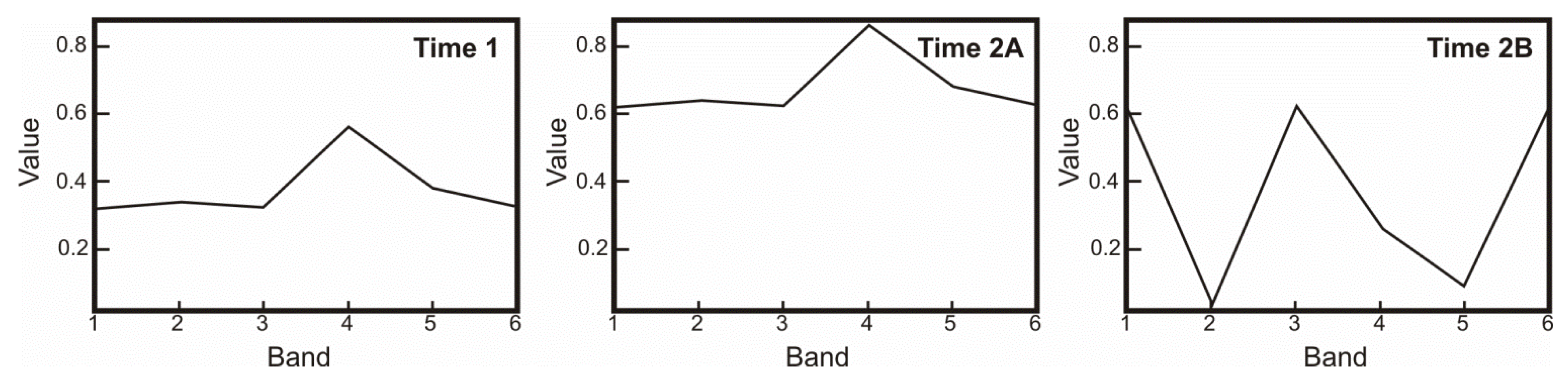
There are important properties that need to be considered when we analyze a measure of change. The major distinction between the methods is their ability to identify shapes or to establish magnitude differences. The distinction between these two properties is illustrated in Figure 5, which compares a curve from time t₁ to two curves from time t₂, (a and b). The distance measure cannot identify the similarity patterns. Thus, the Euclidean distance has the same value of magnitude (0.735) between t₁ and the two curves of t₂ (Figure 5). In contrast, similarity measures easily detect the two spectral shapes. The SCM values demonstrate that t₁ has highest correlation with t_2a (1.0), and negative correlation with t_2b (−0.350). Thus, the diagnostic features of the each material can be clearly described and identified over time.

Figure 5. Comparison of a curve from time 1 (t₁) to two curves from time 2, (t_2a and t_2b): t₁ − t_2a (Euclidian distance, 0.735; and SCM, 1.0); and t₁ − t_2b (Euclidian distance, 0.735; and SCM, −0.350).

Figure 5. Comparison of a curve from time 1 (t₁) to two curves from time 2, (t_2a and t_2b): t₁ − t_2a (Euclidian distance, 0.735; and SCM, 1.0); and t₁ − t_2b (Euclidian distance, 0.735; and SCM, −0.350).

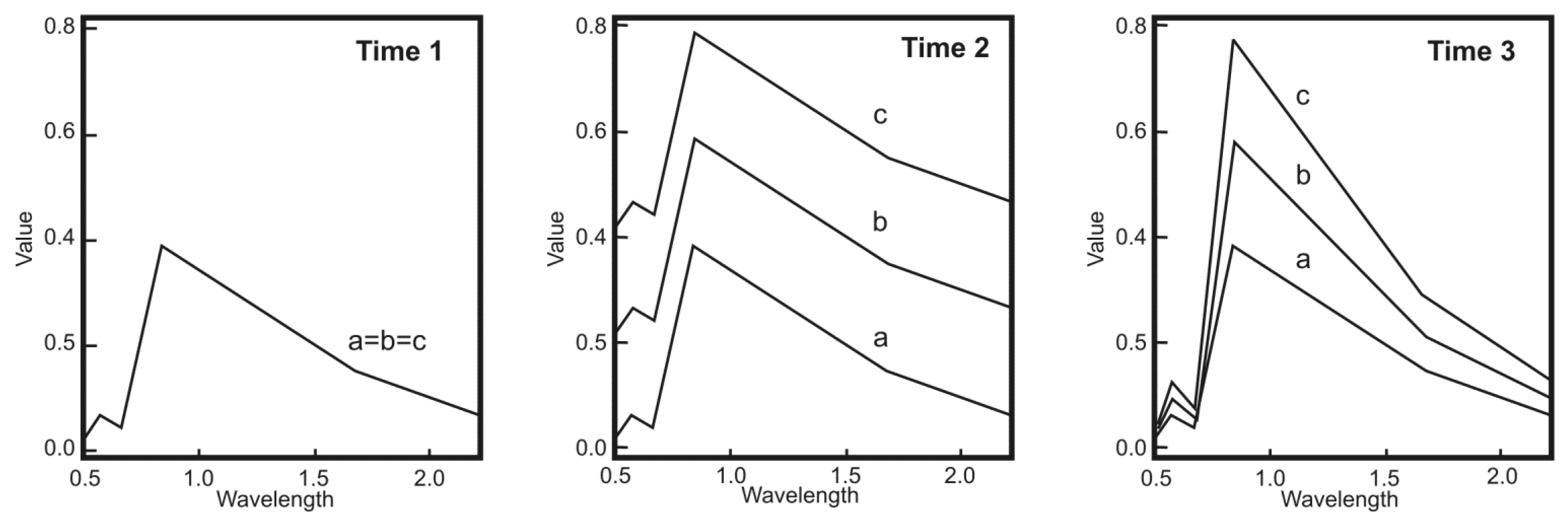
These changes of gain and offset are common among temporal images, due to shading, clouds, and sensor calibration. These properties are demonstrated in Figure 6, which present three spectra from t₁, which are altered by different offset factors at t₂ and gain factors at t₃. The offset values described for t₂ alter both the Euclidian distance (b = 0.48990 and c = 0.9798) and SAM (b = 0.44553 and c = 0.58545). Comparison between t₁ and t₃ shows that the gain factor changes only the Euclidian distance (c = 0.42173 and b = 0.21087) and does not modify SAM (a = b = c = 0) and SCM (a = b = c = 1). Therefore, the SCM method remains unchanged in all situations for which the value equals 1, SAM eliminates the effect of gain, and Euclidean distance is altered by both factors.

Figure 6. Effects of gain and offset changes. Time t₁: equal gain and offset; Time t₂: different offset; and Time t₃: different gain.

Figure 6. Effects of gain and offset changes. Time t₁: equal gain and offset; Time t₂: different offset; and Time t₃: different gain.

One important argument for using the measure of similarity is that the spectral features are maintained independent of gain and offset, allowing us to identify the material composition. However, spectrum normalization is not always desired. Sometimes a simple change of gain and offset can represent relevant change to the study, as is the case for vegetation spectra.

The Mahalanobis distance was not evaluated because it depends on values of the individual covariance image, and does not allow a direct comparison from spectra. However, this measure is also influenced by gain and offset.

2.6. Accuracy Assessment

The critical part of CVA method is to select the appropriate threshold value of the distance or similarity measure to represent the boundary between “change” and “no-change” information. The thresholds are usually determined empirically and depend on the image and the analyst’s experience. For threshold-value determination, we developed an algorithm similar with Fung and LeDrew method [26]. The definition of optimal threshold value is obtained by comparing with a classified map elaborated from field validation and accurate interpretation of imagery of higher spatial resolution. The reference area must be characterized as representative and not too large. Thus, the best threshold value is identified from the maximum Kappa coefficient or Overall accuracy, commonly used to assess accuracy [27,28,29]. The overall accuracy is calculated by summing the number of pixels classified correctly and dividing by the total number of pixels. The Kappa coefficient (Κ) is an accuracy measure of the classification described by following equation:

$$K=\frac{m{\displaystyle \sum _{i=1}^r{s}_{ii}-{\displaystyle \sum _{i=1}^r{s}_{i+}{s}_{+i}}}}{m^2-{\displaystyle \sum _{i=1}^r{s}_{i+}{s}_{+i}}}$$

(8)

where “r” is the number of rows in the error matrix, “s_ii” is the number of observation on row “i” and column “i”, “s_i+” and “s_+i” are thus the marginal totals on row “i” and column “i”, respectively, and “m” is the total number of observations. Once the threshold value is defined from reference area, it can be applied to the entire image.

3. Results

3.1. Image Analysis

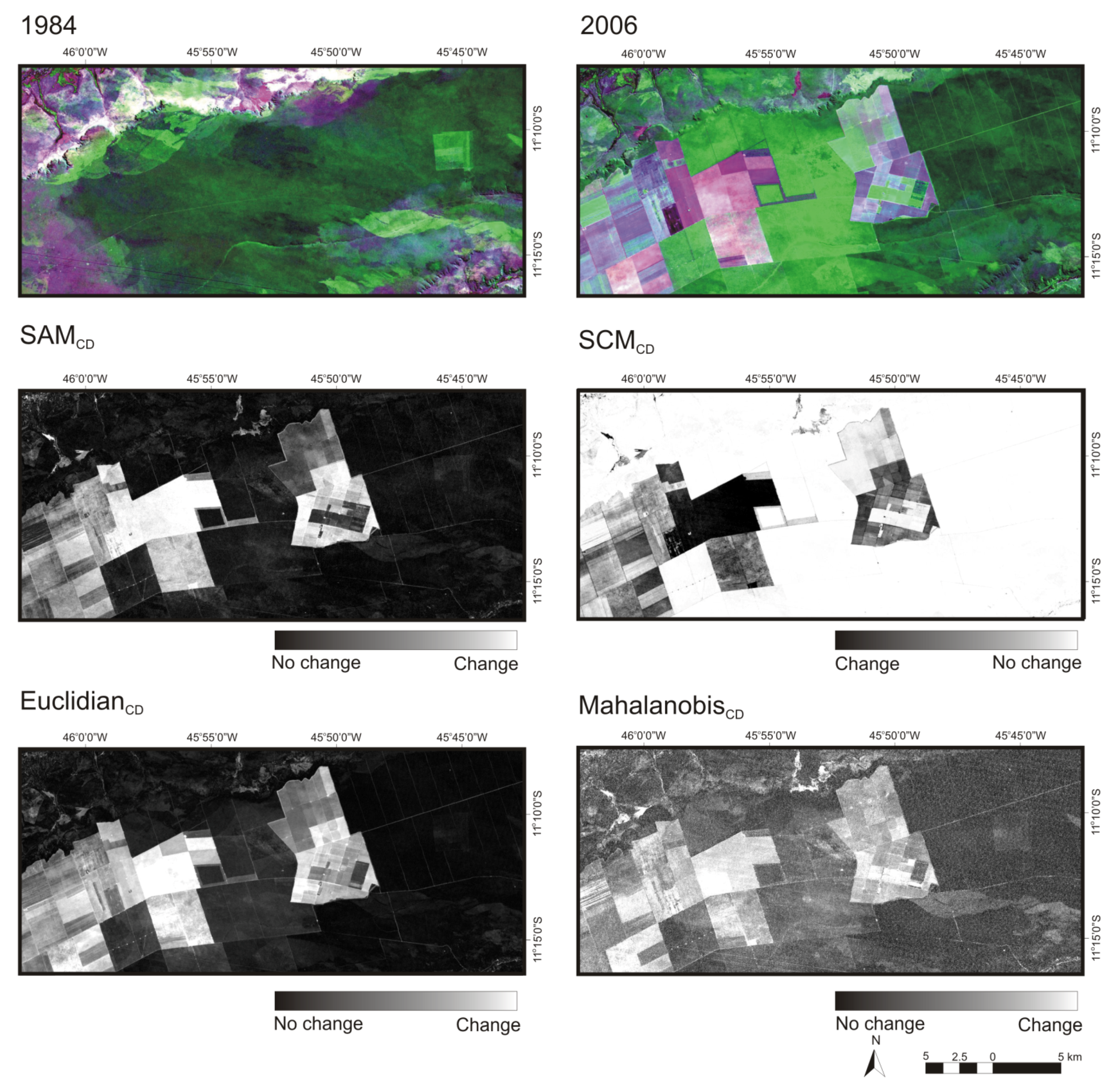
The resulting images of the four methods differ in the grayscale (Figure 7). In SCM_CD method the darker cells indicate a lower correlation between the temporal pixel pair while the lighter cells indicate a higher correlation. Due to the mathematical formulation, SAM_CD, Euclidian distance and Mahalanobis distance in comparison with SCM_CD method are represented by an inverted grayscale legend, i.e., the darker cells indicate high correlation.

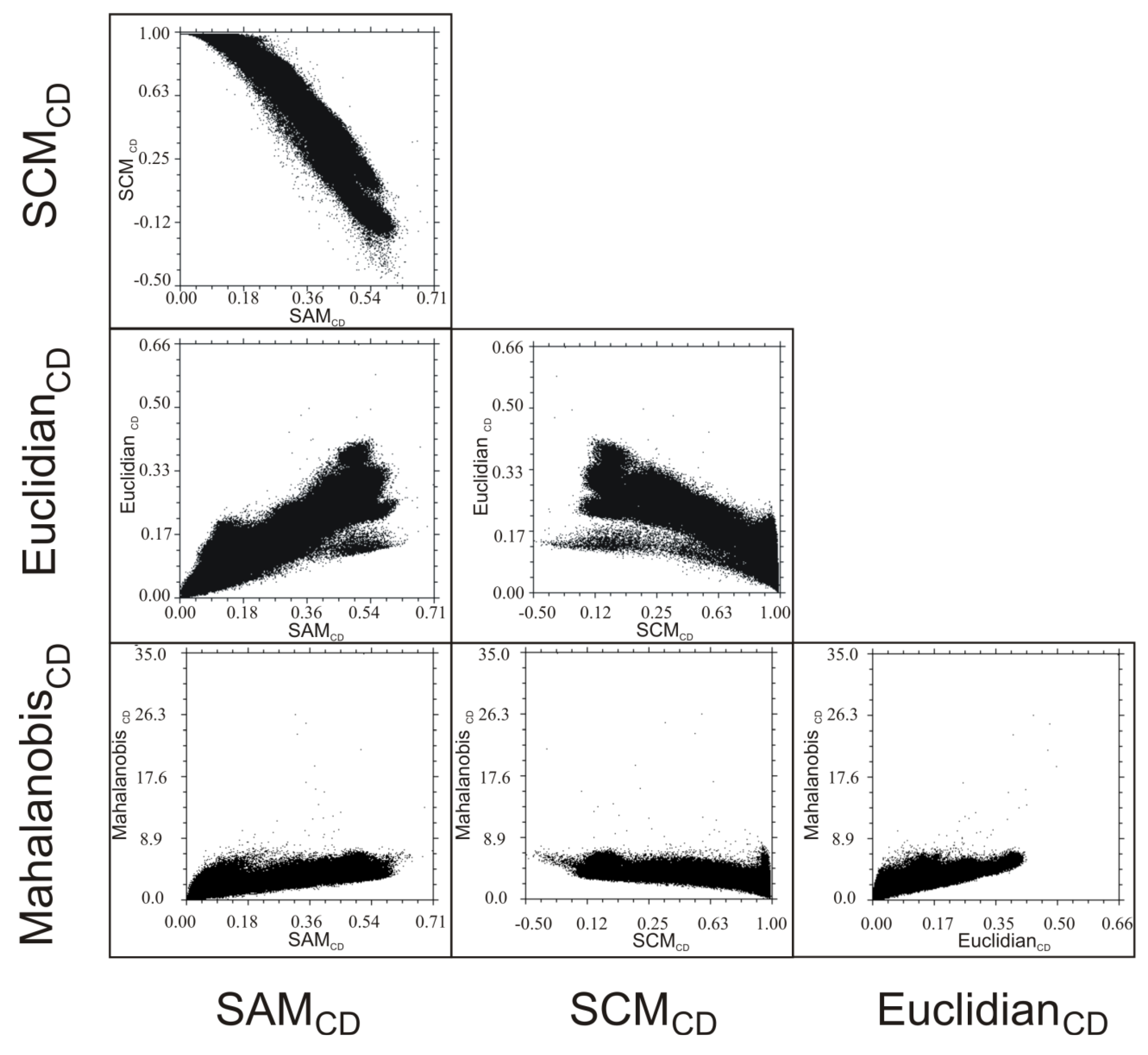
In order to emphasize the nuances among the methods, Figure 8 shows scatterplots between the measure images. Among the similarity measures, SAM_CD in relation to SCM_CD has an analogous distribution and the data dispersion is caused mainly by an offset factor. So a certain value of SCM_CD can contain different values of SAM_CD, which vary according to the increase in the offset factor.

The distance measures in the scatterplots have a broader distribution because of greater susceptibility to the effects of gain and offset. The Mahalanobis distance has significant differentiation in relation to the Euclidian distance and other methods due to the normalization used to compensate the variations between different bands. Thus, the Mahalanobis distance increases the importance of bands having little variation of reflectance, usually in visible bands. Eventually, this procedure may increase noise in image results. The scatterplot between the distances measures show an increasing dispersion from the origin caused by the contributions of different bands.

Figure 7. Images resulting from the change-detection (CD) methods. (a) 1984 input image; (b) 2006 input image; (c) Spectral Angle Mapper (SAM_CD); (d) Spectral Correlation Mapper (SCM_CD); (e) Euclidian distance; and (f) Mahalanobis distance.

Figure 7. Images resulting from the change-detection (CD) methods. (a) 1984 input image; (b) 2006 input image; (c) Spectral Angle Mapper (SAM_CD); (d) Spectral Correlation Mapper (SCM_CD); (e) Euclidian distance; and (f) Mahalanobis distance.

An important difference between the methods is the capacity of differentiation of vegetation change. The reflectance spectra of most plant canopies are dominated by green leaves. These are characterized by diagnostic absorption feature of the photosynthetic pigments (chlorophylls and carotenoids) in the visible (0.4 to 0.7 μm) [30,31], refractive-index discontinuities in the spongy mesophyll, which causes a near-infrared light (0.7 to 1.3 μm) to be dispersed [31,32], and water absorption in the shortwave infrared (1.3 to 2.5 μm).

Figure 8. Bivariate scatter diagrams for change-detection (CD) measure images: Spectral Angle Mapper (SAM_CD), Spectral Correlation Mapper (SCM_CD); Euclidian distance; and Mahalanobis distance.

Figure 8. Bivariate scatter diagrams for change-detection (CD) measure images: Spectral Angle Mapper (SAM_CD), Spectral Correlation Mapper (SCM_CD); Euclidian distance; and Mahalanobis distance.

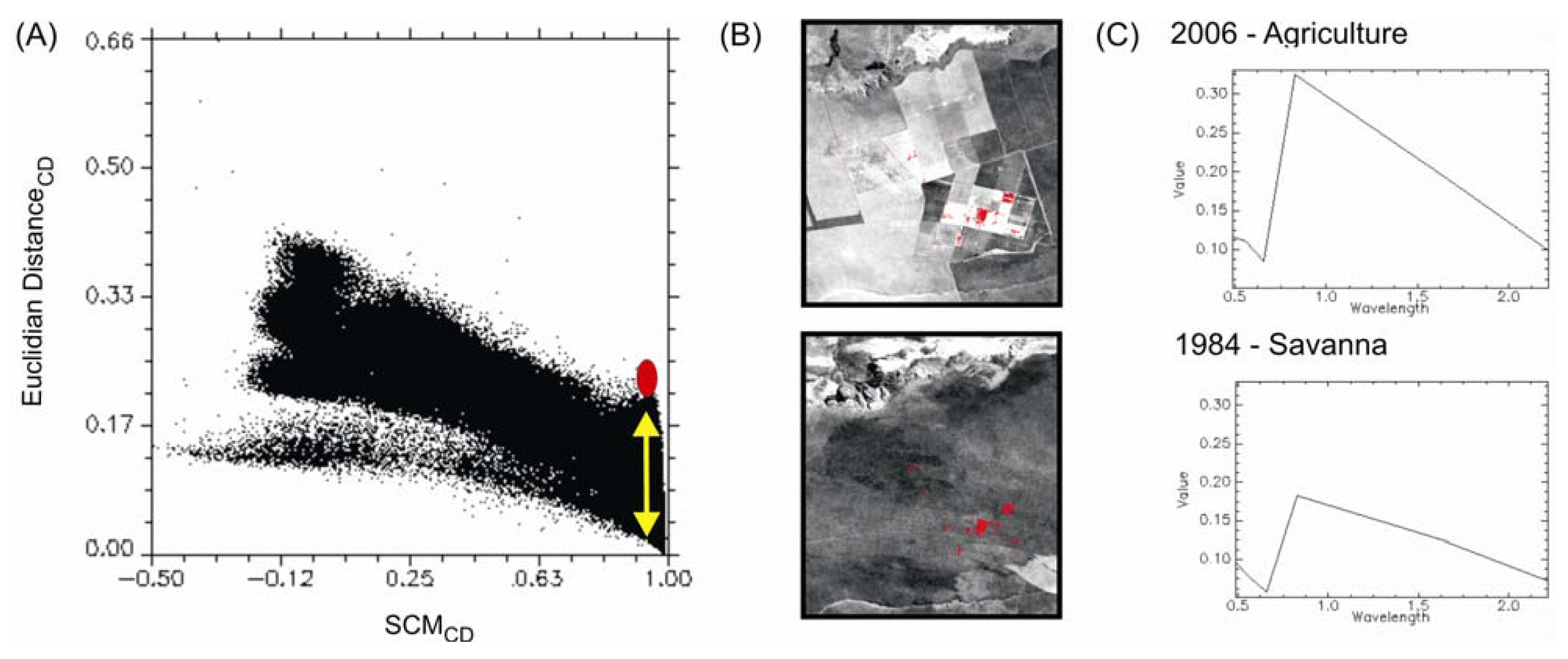
In the study area there are changes of savanna to agricultural crops, where both are characterized by photosynthetic vegetation (PV). The differences among these temporal spectra are predominantly in the reflectance amplitudes easily detected by the distance measures. However the similarity measures based on spectral matching identify the same PV features and consider them too close to each other to represent change. Thus, the temporal changes from the PV spectra between the agriculture and savanna can be captured only with high threshold values for SCM_CD and low threshold values for SAM_CD.

In order to illustrate this, Figure 9 shows a red spot in the scatterplot relating SCM_CD and Euclidian distance with their locations in both the 1984 and 2006 images, and their average spectrum. The pixels along the yellow arrow represent the same value for SCM_CD methods. The spectra in savanna in 1984 and agriculture in 2006 have the same features, and the differences are just in gain and offset. Therefore, the important transition from savanna to agriculture is hard to capture. The distance measures have errors as shown in Figure 5 where the same distance values correspond to curves without similarity. This is identified by similarity measures.

Figure 9. (a) Spectral Correlation Mapper for change detection (SCM_CD) versus Euclidian distance scatterplot showing a data point having a high SCM value and low Euclidian distance (red spot); (b) 1984 and 2006 images with points having the (SCM_CD, Euclidian distance) tagged as the red spot in (a); and (c) their average spectra.

Figure 9. (a) Spectral Correlation Mapper for change detection (SCM_CD) versus Euclidian distance scatterplot showing a data point having a high SCM value and low Euclidian distance (red spot); (b) 1984 and 2006 images with points having the (SCM_CD, Euclidian distance) tagged as the red spot in (a); and (c) their average spectra.

3.2. Accuracy Assessment Results

The reference map was built from the visual interpretation of Panchromatic Remote Sensing Instruments for Stereo Mapping (PRISM) sensor aboard the Advanced Land Observing Satellite (ALOS) satellite of Japan Aerospace Exploration Agency (JAXA) with high spatial resolution (2.5 m); detailed field validation; and Landsat-TM temporal color composite images [33,34]. Despite the restriction of ALOS images to a one-year period, in this study they allow the detection of changes between 1984 and 2006, because in 1984 it hadn’t yet been agricultural inroads.

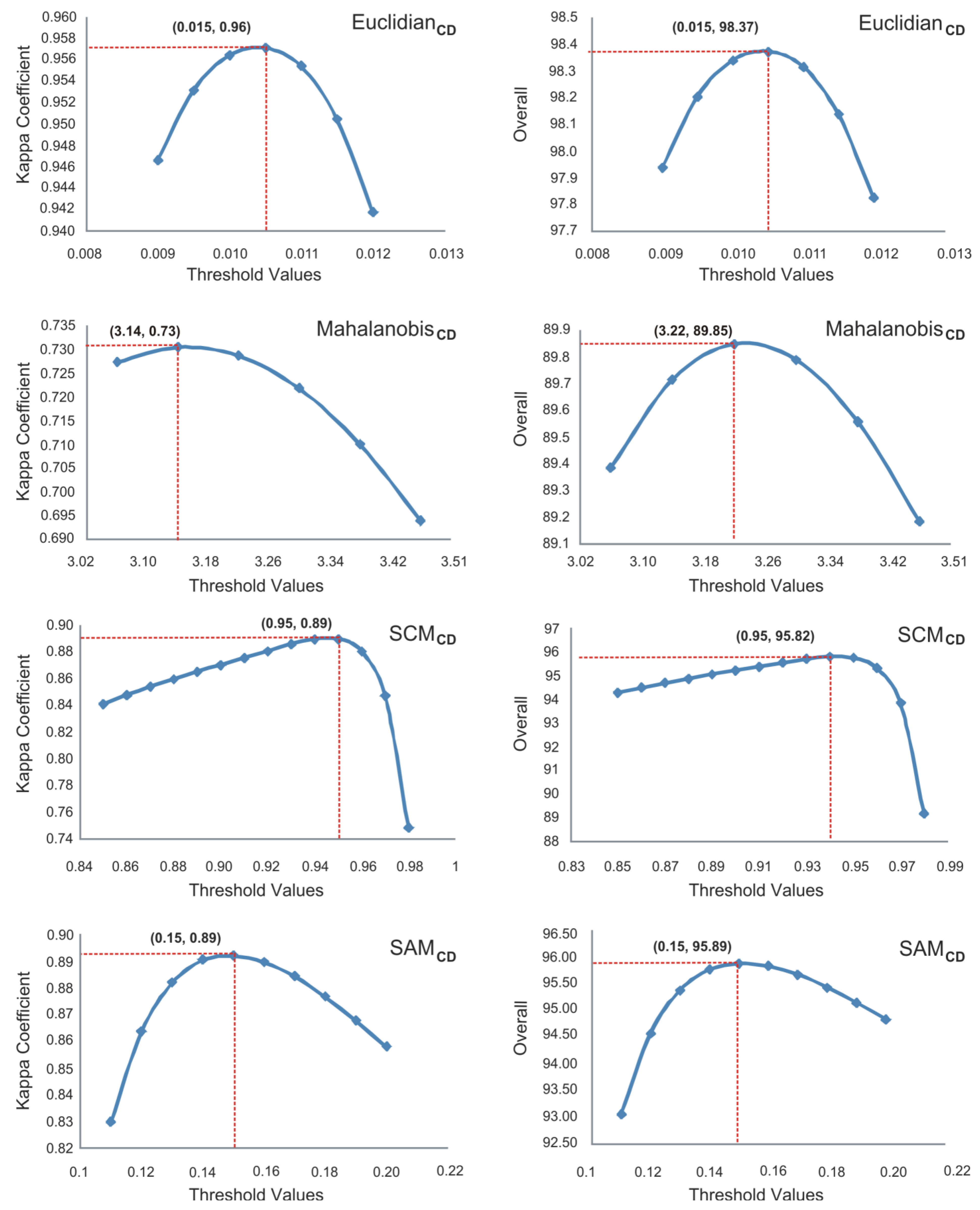
The measure images were classified using a threshold value. The definition of the best threshold for each method was from the best fit (i.e., Kappa coefficient or Overall accuracy) with the entire reference map. Therefore a set of classified images with different thresholds were tested to obtain the optimal value. Figure 10 shows the graph of Overall accuracy and Kappa coefficient relative to threshold values for each method. The best-fit results are obtained from Euclidian distance with 0.96 of Kappa coefficient and 98.37 of Overall accuracy. The similarity measures SCM_CD and SAM_CD show similar values of 0.89 for Kappa coefficient and values of 95.8 for Overall accuracy. In contrast, the worst results are Mahalanobis distance with 0.73 of Kappa coefficient and 89.85 of Overall accuracy.

The similarity measures results show a high correlation percentage in the savanna converted to agriculture where both are covered by PV. This fundamental problem is not really an error in the context of this study, since its purpose is to identify changes in surface composition. Consequently, forcing the similarity measures to match the land-use map is not necessarily or always the best strategy. An appropriate methodology for defining the similarity measure thresholds is to adapt the land-use map, disregarding changes in PV areas. Thus, the values of overall accuracy and Kappa coefficient for SAM_CD are 97.62 and 0.93, respectively, and the best fit threshold is 0.18; and for SCM_CD the values are 98.20 and 0.95, respectively, and the best fit threshold is 0.92. The two methods show a significant improvement.

Figure 10. Identification of the optimal threshold values for assessing change images made with the Euclidian distance, Mahalanobis distance, Spectral Correlation Mapper (SCM_CD) and Spectral Angle Mapper (SAM_CD) algorithms from the highest Kappa coefficient and Overall accuracy.

Figure 10. Identification of the optimal threshold values for assessing change images made with the Euclidian distance, Mahalanobis distance, Spectral Correlation Mapper (SCM_CD) and Spectral Angle Mapper (SAM_CD) algorithms from the highest Kappa coefficient and Overall accuracy.

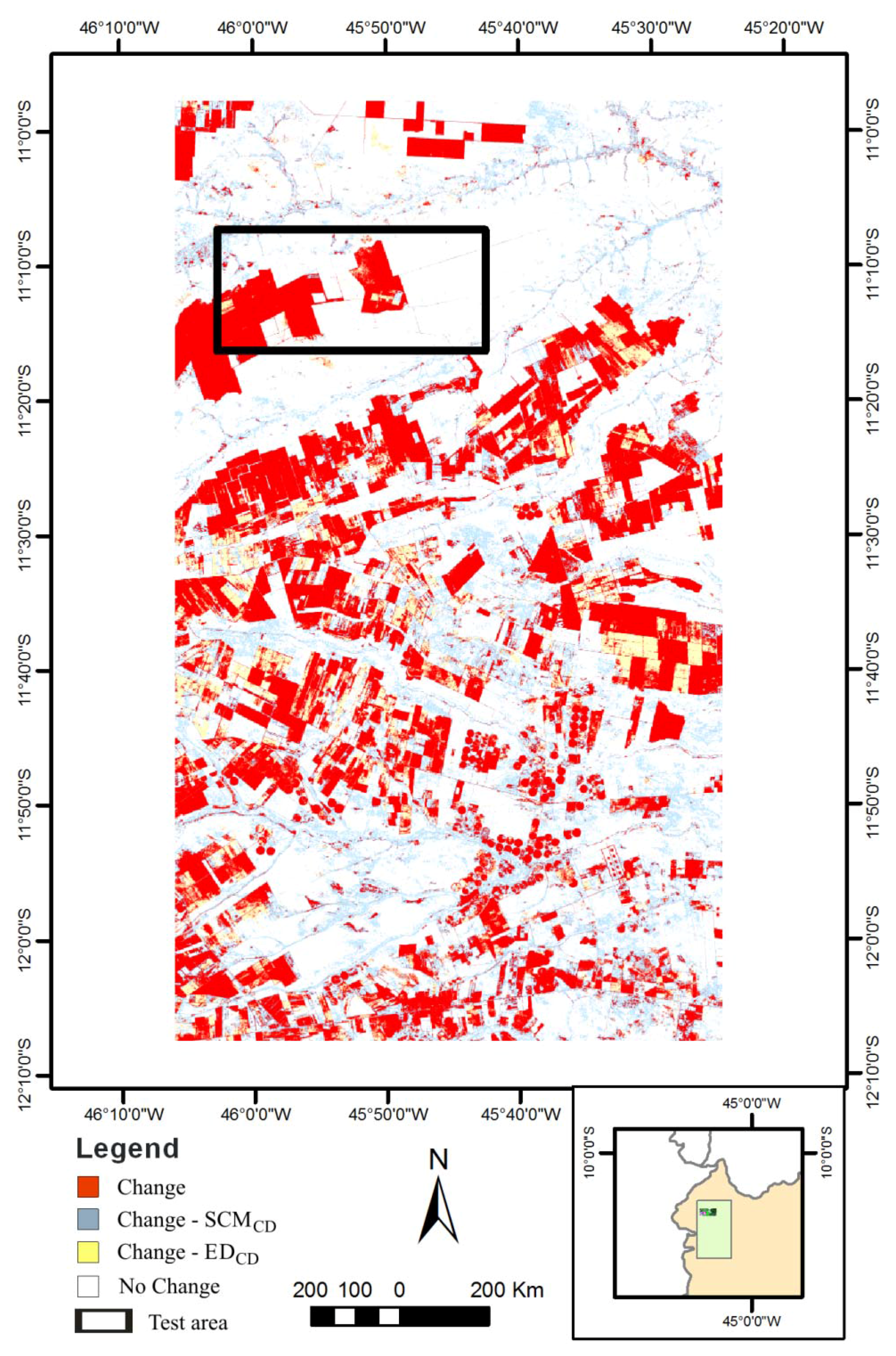
Threshold values set for the four methods in the test area (Figure 3) were applied to the entire region of Western Bahia (Figure 11). Thus, the statistical values identified in the test area, which have a validation with field work, are applied to other areas with similar characteristics. Change detection by distance and similarity measures are compared using the cross-tabulation method. Figure 11 presents a relationship between the two most different measures, Euclidian distance and SCM_CD.

Figure 11. Change image made by integrating the Spectral Correlation Mapper (SCM_CD) and Euclidian distance (ED_CD) measures. Considering the statistical results obtained in this test area shown in Figure 3.

Figure 11. Change image made by integrating the Spectral Correlation Mapper (SCM_CD) and Euclidian distance (ED_CD) measures. Considering the statistical results obtained in this test area shown in Figure 3.

Most of the area presents the same classification for both methods: change (red areas) and no change (white areas). However, some areas presented divergences. Areas detected by SCM_CD and disregarded by Euclidian distance have spectra with different shapes at different times, and typically low albedo along rivers due to hydromorphic soils (blue areas in Figure 11). On the other hand, the changes mapped by Euclidian distance but disregarded by SCM_CD are vegetated areas where the temporal spectra have the same shape and different gain and offset (yellow areas in Figure 11). Thus, the results demonstrate that the methods are complementary and should be used together for the best change detection results.

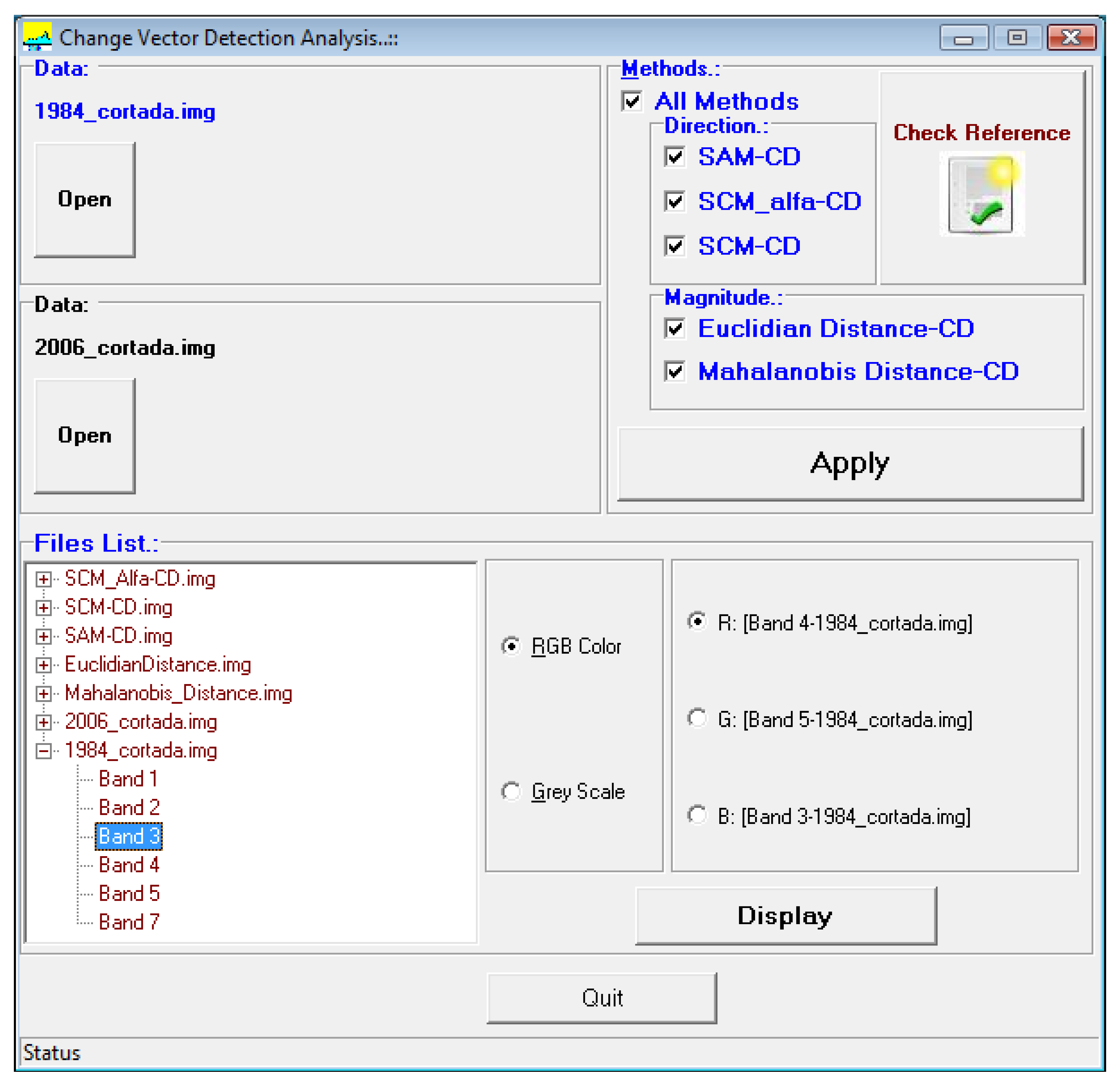
3.3. Program

The methods discussed above are available in user-friendly software developed in C++ language. The main functions of the program are organized in the main window interface which contains the image input boxes, CVA method options and image display (Figure 12).

Figure 12. Main window interface contains image input boxes, CVA method functions and image display.

Figure 12. Main window interface contains image input boxes, CVA method functions and image display.

The program reads general raster data stored as an interleaved binary stream of bytes in the Band Sequential Format (BSQ) and Band Interleaved by Pixel Format (BIP). Each image is accompanied by a header file in ASCII (text) containing information to read data file, such as: sample numbers, line numbers, bands, interleave code (BIP or BSQ) and data type (byte, signed and unsigned integer, long integer, floating point, 64-bit integer, unsigned 64-bit integer). This configuration combining image and header file allows versatility in the use of different image formats. When the user tries to open an image without the header file, an interface requesting the necessary information about the input image structure automatically appears.

Input files are required for the two temporal images ($X^{t_1}$ and $X^{t_2}$), which must be co-registered and have the same number of rows, columns and bands. Four options for change-detection measure are provided: (1) Euclidian distance; (2) Mahalanobis distance; (3) SAM_CD, and (4) SCM_CD. The user can select the measures deemed appropriate.

The calculated results are gray scale images depicting the measure values, which describe the amount of temporal change between successive scenes at times t₁ and t₂. All inputs and results are shown in the File List, so it is possible to visualize them by choosing “Gray Scale” or “RGB” composite (Figure 12). 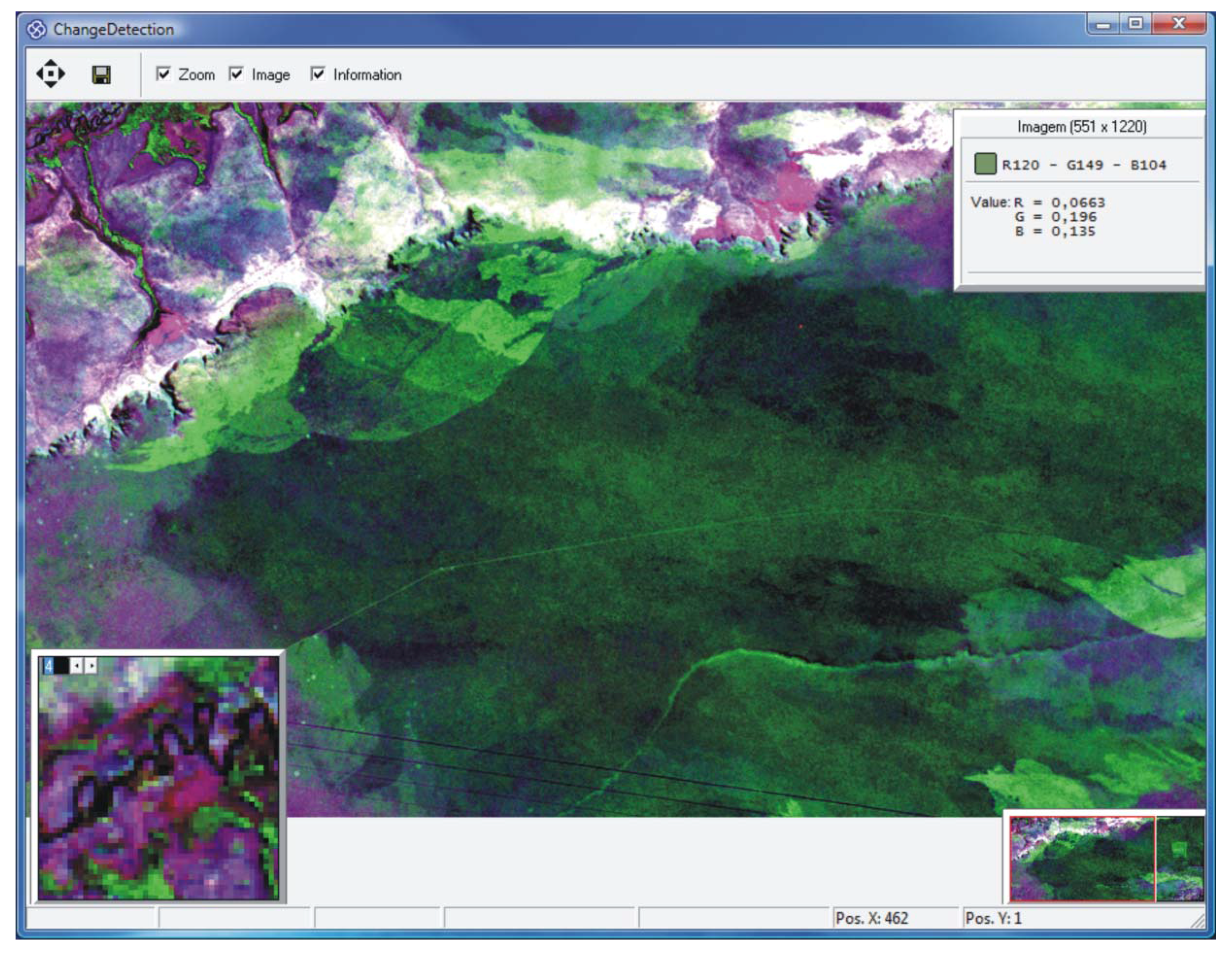The display interface provides basic functions for images visualization such as zoom areas and pixel values (Figure 13). Moreover, the results (output files) can be read from other viewers of binary images.

Figure 13. Display interface with basic functions for image visualization. Color composition of TM-Landsat image at 1986 (RGB-TM bands 3, 4, and 5).

Figure 13. Display interface with basic functions for image visualization. Color composition of TM-Landsat image at 1986 (RGB-TM bands 3, 4, and 5).

4. Conclusion

The CVA [1] method generates two components: magnitude and direction of change. The direction of change for n-dimensional multispectral data is difficult to calculate and interpret. The procedure most commonly used is the direction cosine method [5,6,7], but this generates the same number of output images that the input data and has a complex interpretation. This paper proposes a new alternative to calculate the direction of change using the angle between temporal vectors. This approach adopted spectral similarity measures (Spectral Angle Mapper, SAM_CD, and Spectral Correlation Mapper, SCM_CD) to estimate the direction of change. This proposed procedure has the following advantages: (1) the information is synthesized in only one band, (2) the resulting image has a scale value that indicates the degree of change, (3) the mathematical formulations are widely used in spectral classifiers, (4) emphasizes the shapes of spectral curves, and (5) these methods are insensitive to illumination variation. Alternatively, the similarity metric images can be used in conjunction with the direction cosine images in future works.

The main difference between the two similarity metrics used is that SCM_CD shows perfect similarity despite the differences in basal expression level (offset) and scale (gain) while SAM_CD only annuls the offset attribute. In addition, the CVA using similarity metric enables a relative radiometric correction, pixel by pixel. Processing by pixel spectrum can be an advantage in change-detection, especially when there are environmental differences restricted to only one time and one part of the image, such as a cloud shadow. A possible limitation of similarity metrics is in places with very low albedo with noise domain.

Since the conception of CVA, the magnitude component has been obtained using Euclidean distance. However, Mahalanobis distance is also useful for change-detection, although it has not been compared with the CVA method. Thus, in this paper these two distances were compared to estimate the magnitude component. The main difference between the methods is that the Mahalanobis distance approach performs band normalization. Moreover, Mahalanobis distance depends on the covariance matrix of a multi-band image, resulting in a specific linear transformation for each image set. This characteristic limits the comparison of the Mahalanobis method results in different areas. In this study case, the distance measure that had the best performance was Euclidean distance, while for the similarity measures there was a slight preference for SAM_CD.

There is no one measure type (distance or similarity) that is better than others in every situation. This is because different measures have particular properties, some of which may be desirable for certain applications but not for others. Measures of distance (magnitude) and spectral angle (shape) contain complementary information and using both, where appropriate, increases the probability of performing accurate analyses of change.

This algorithm is different from the other proposition [35,36,37], which use similarity and distance measures to a spatial moving window in two times. In this paper the proposition is not a spatial comparison, considering a mask (e.g., 3 × 3 pixels). However, this spectral approach shown in this article may be linked to a spatial approach in future work.