Field Spectroscopy for Assisting Water Quality Monitoring and Assessment in Water Treatment Reservoirs Using Atmospheric Corrected Satellite Remotely Sensed Imagery

Abstract

The overall objective of this study was to use field spectro-radiometers for finding possible spectral regions in which chlorophyll-a (Chl-a) and particulate organic carbon (POC) could be identified so as to assist the assessment and monitoring of water quality using satellite remote sensing technology. This paper presents the methodology adopted in this study which is based on the application of linear regression analysis between the mean reflectance values (measured with the GER1500 field spectro-radiometer) across the spectrum and the concentrations of chlorophyll-a (µg/L) and POC (µg/L) acquired simultaneously on the same day and time in the Lower Thames Valley in West London (U.K.) from old campaigns. Each regression model (512 in total) corresponded to a measured wavelength of the GER1500 field spectro-radiometer. The achieved correlations presented as r² against wavelength, indicate the regions with high correlation values for both water quality variables. Based on the results from this study and by matching the spectral bands of the field spectro-radiometer with those of the Landsat TM satellite sensor (or any other sensor), it has been found that suitable spectral regions for monitoring water quality in water treatment reservoirs are the following: for chlorophyll-a, the spectral region of 0.45–0.52 μm (TM band 1), and for POC, the region 0.52–0.60 μm (TM bands 1 and 2). Then 12 atmospheric corrected Landsat TM/ETM+ band 1 images acquired from 2001 to 2010 were used for validation purposes to retrieve the Chl-a concentrations.

1. Introduction

Field spectroscopy has previously been applied to obtain radiance, irradiance and reflectance values of freshwater, sea-water and pure water [1,2,3,4,5,6,7,8,9,10,11,12]. Spectrometers or spectro-radiometers are widely used to collect spectral data [13]. Dekker [14] found that the reflectance spectrum of inland waters is centered on the 500 nm–700 nm spectral region [15]. This, therefore, suggests that information about the quality of inland waters can be best obtained in the green to near-infrared (NIR) range.

Most of the published works, in which several satellite image data such as Landsat, SPOT, MODIS etc. have been reportedly used for monitoring inland water quality studies, use sampling measurements in combination with the digital imagery [16,17,18] Statistical techniques have been used to investigate the correlation between spectral wave bands or waveband combinations and the desired water quality parameters [6,8,9,18]. Hence, predictive equations for water quality parameters have been established after these correlations have been determined. It has been shown by several other researchers, who studied the actual relationship between water properties (i.e., water quality) and satellite data for several types of water bodies, that satellite remote sensing techniques show more important advantages than traditional sampling [15,18,19,20,21,22,23]. Indeed, He et al. [18] reported that with the development of remote sensing techniques, water quality monitoring based on such remote sensing methods has become accessible and very efficient. However, the major difficulty is to find in advance the optimal or suitable spectral region in which the water quality parameters should be retrieved [24] so as to avoid any errors in the development of predictive equations.

Previous studies show that the extraction of historic and up-to-date water quality data from Landsat TM satellite images, coupled with existing data collection efforts, can facilitate the development of comprehensive regional databases that can be used to evaluate water quality trends over time and space (e.g., [22]). Although several satellite remote sensing systems have been used for water quality assessment and water quality parameter determination, generally the relatively low cost, temporal coverage and data availability of the Landsat system make it particularly useful for studies related to the monitoring and assessment of water quality in inland water bodies. It has been shown in other studies that the retrieval models with Landsat-5 TM data could meet the accuracy requirements of routine water quality monitoring on reservoir for algae content, turbidity etc., as they could be retrieved within a mean relative error (MRE) of 20% [18]. The accuracies of water quality retrieval could be greatly improved under a support of new remote sensing data with higher spectral and spatial resolutions than Landsat TM/ETM pixel size [18]. For large water bodies such as dams or water treatment reservoirs, the effect of the medium sensor resolution i.e., 30 m × 30 m is not a very significant parameter. For pixels of spatial resolution of less than 30 m the assumption of a nearly homogeneous water body is reasonable.

The research objectives of this study are the following:

• to identify the spectral region in which chlorophyll-a (Chl-a) and particulate organic carbon (POC) can be retrieved using field spectroscopy;
• to develop a novel methodology to measure the reflectance at the water surface using field spectroscopy;
• to develop regression models based upon the spectral features to monitor the water quality in large water treatment reservoirs in West London using satellite imagery acquired during water sampling;
• to use such regression models for further testing using atmospheric corrected satellite imagery.

2. Materials and Methods

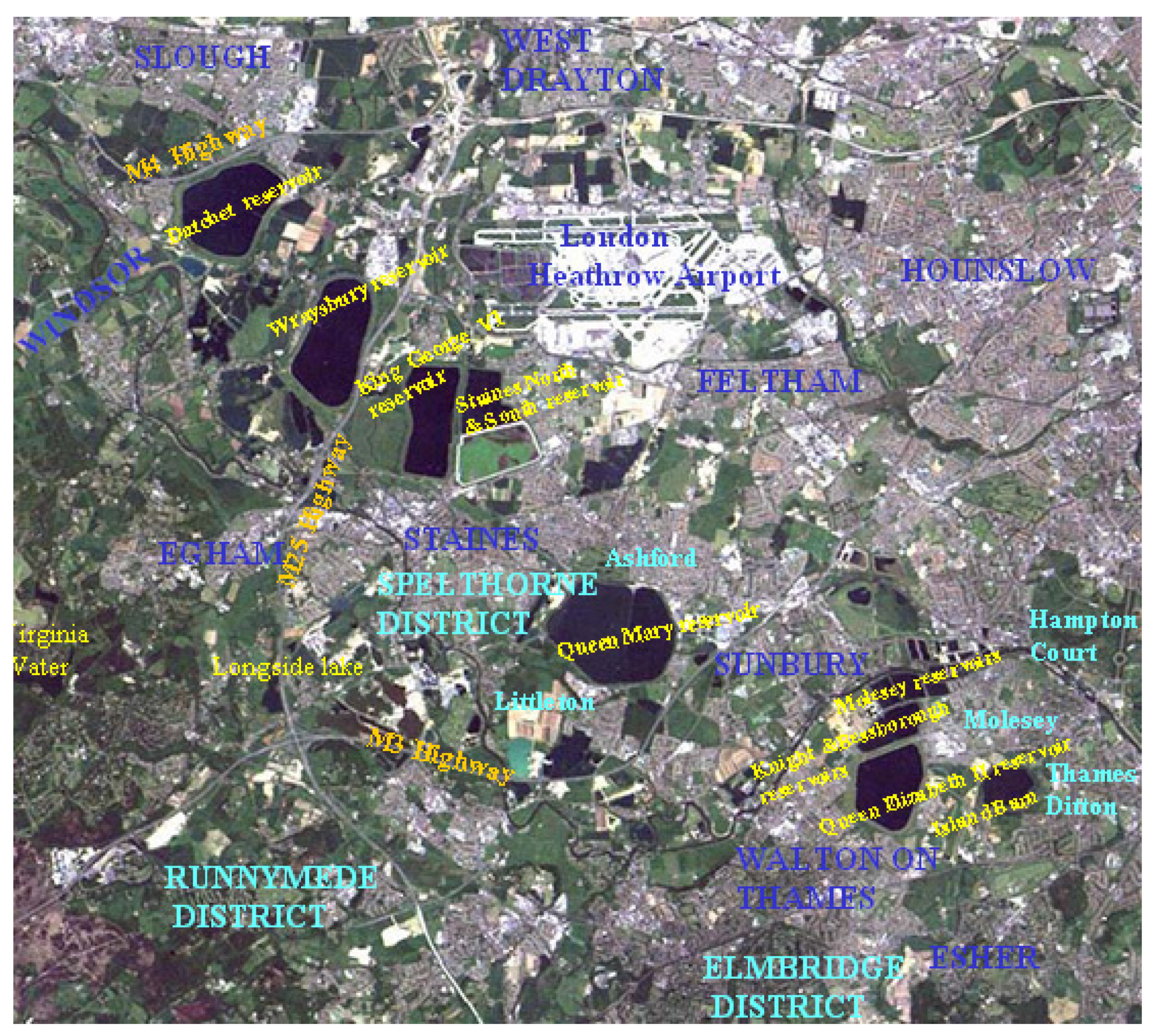
2.1. Study Area

The study area is located to the south and the west of London Heathrow Airport in the UK. It includes many inland water bodies such as reservoirs, rivers, lakes and ponds. Emphasis has been given to the larger reservoirs in the Lower Thames Valley (see Figure 1). The Lower Thames Valley reservoirs are characterized as eutrophic and are used for a number of purposes, such as for storage of water, as the first stage of potable water treatment, and for recreational purposes. Despite the fact that cloud cover is a major problem in this area [25], restricting the adequate number of satellite remotely sensed images that can be obtained in any particular year of study, it has been found that satellite remote sensing and especially Landsat TM imagery can be a useful tool for monitoring water quality in such reservoirs as well as to assist the managing company to locate new sampling points based on the synoptic assessment of satellite images [25,26].

Figure 1. Partial scene of the Heathrow area and Lower Thames Valley reservoirs (Landsat-5 TM image acquired on 2 June 1985 displayed in true color combination with key locations and feature labeled).

Figure 1. Partial scene of the Heathrow area and Lower Thames Valley reservoirs (Landsat-5 TM image acquired on 2 June 1985 displayed in true color combination with key locations and feature labeled).

2.2. Resources

A powered boat, a GER1500 spectro-radiometer with associated equipment and a GPS were used in the measurement campaign. The major task of the ground measurements was to determine the reflectance of the reservoir at the water surface, i.e., at approximately zero depth.

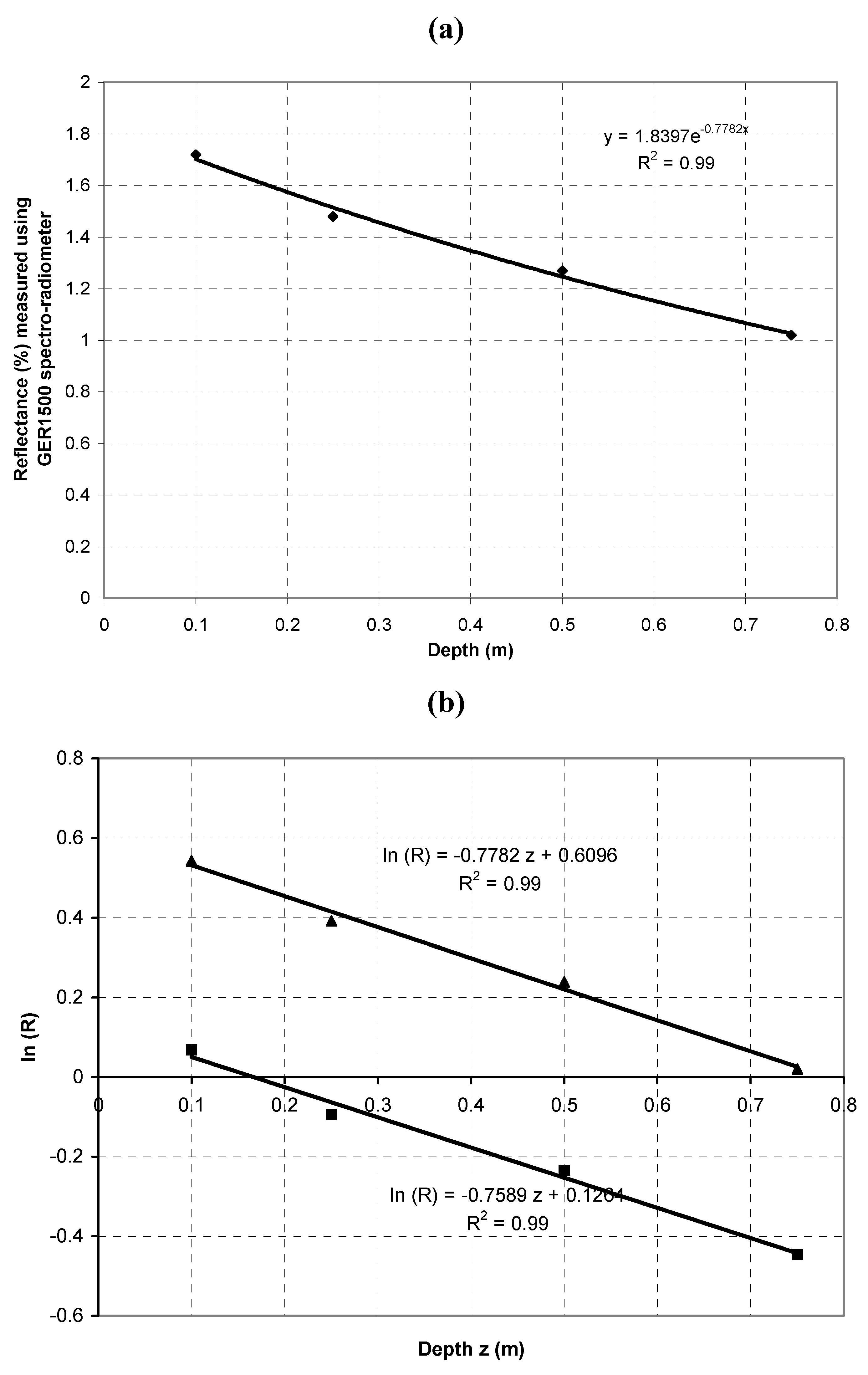
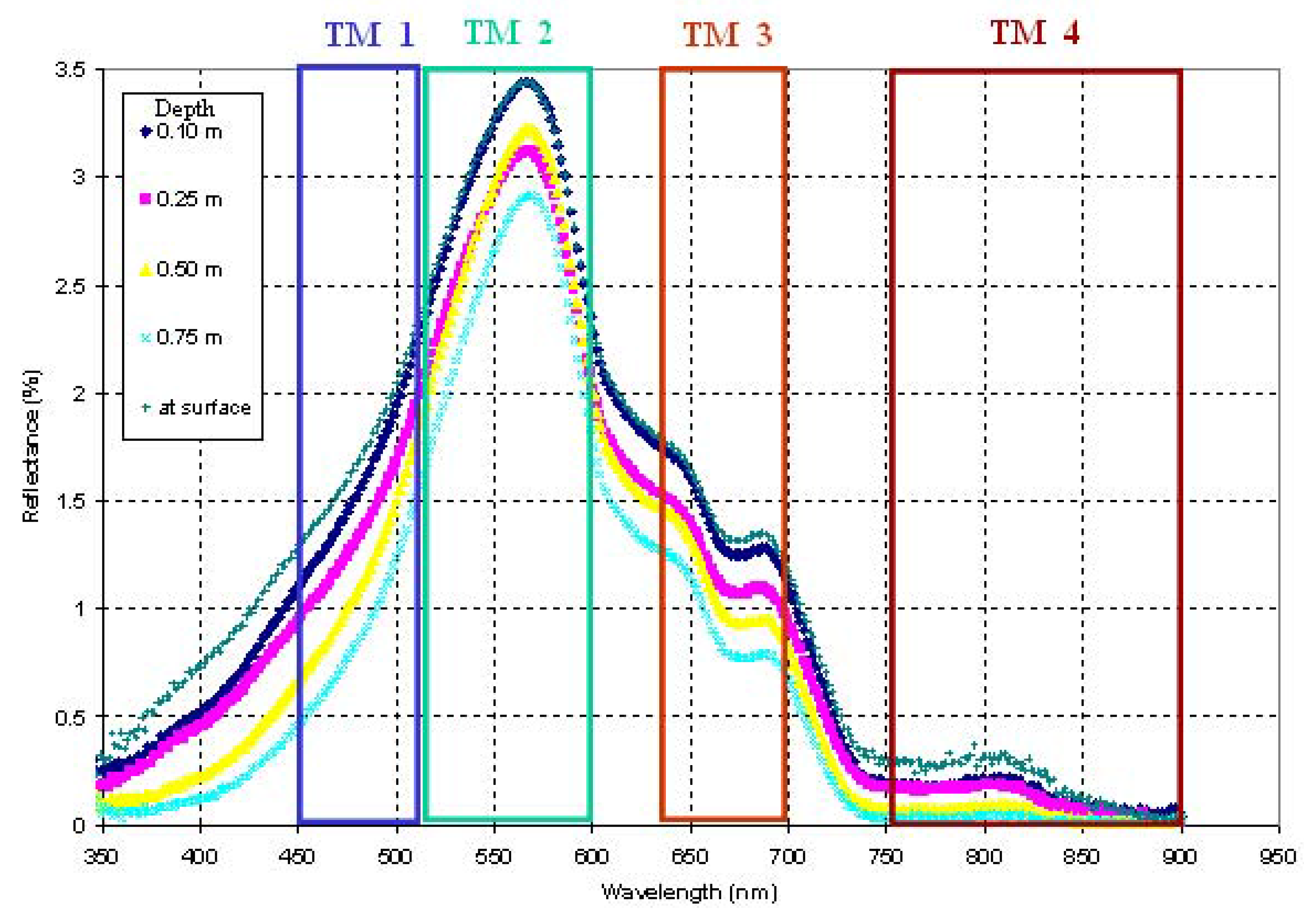
2.3. Spectro-Radiometric Measurements

Spectral reflectance measurements were carried out using a GER1500-spectroradiometer covering the UV, visible and near infrared. This spectro-radiometer has a full width half maximum (FWHM) of 3 nm and covers the spectral range from 350 nm to 1,050 nm.

In this study the method using a white reference panel described by Milton and McCloy was used [27,28,29,30]. The GER1500 was used to acquire measurements on the target (water treatment reservoir) and on the control panel. By applying the ratio of the reflected radiance from the target to the reflected radiance from the panel and by taking into account the control panel correction, the reflectance of the target was obtained [4].

A new approach for retrieving the water reflectance at the surface was developed based on the practical use of the GER1500 field spectro-radiometer mounted with a fiber-optic probe and the theoretical formulation of the light attenuation in water medium. This method is based on the assumption that the study is concentrated on the surface of the reservoir and any other scattering effects are ignored; that was the reason that the diffuser instrument was not used on the GER1500 field spectro-radiometer. The first task was to decide the appropriate depths at which to place the fiber-optic probe into the water. It was decided after several trial measurements [26] to take data at depths of 0 (approximately) up to 1 m.

The collection of spectro-radiometric data was performed at a number of locations during an extensive measurement campaign on the Lower Thames Valley water treatment reservoirs.

The new approach adopted in this study for retrieving the surface reflectance was developed based on the use of the basic light attenuation equation. Absorption and scattering reduce the intensity of the radiance distribution. Also, scattering processes change the directional distribution of the light intensity. Bukata et al. [31] provided the basic theory in which Equation (1) is derived. Any errors caused by the volumetric scattering in the water body are ignored since they are found to be non-significant for turbid waters and the reflected radiance is considered to be concentrated on the surface of the reservoir [18,31].

For every wavelength, the reflectance (ln $R_z$) against depth (z) was plotted based on Equation (1):

$$\ln R_z=\ln R_0-K.z$$

(1)

where

• R_z is the reflectance at a depth z
• R₀ is the reflectance at zero depth
• K is the irradiance attenuation coefficient or vertical extinction coefficient.

The intercept, which represents the required surface reflectance, was determined by extrapolation. The y-intercept for every plot represents the estimated surface reflectance. For example, Figure 2 shows the linear relationship presented in Equation (1) for four different wavelengths. Those readings in which the deployment of the probe was not vertical (or due to “rolling” of the boat), did not follow the Beer’s Law linearity, were rejected and were not taken into account in further analyses.

Figure 2. (a) The exponential plot according to Beer’s Law is validated. For example, by relating reflectance values (R) acquired on 26 September 1998 at 10:11 GMT with depth at 490 nm, the results show a general agreement with the theoretical exponential plot; (b) The required surface reflectance was found by plotting the ln(R) against depth (for example at 490 nm and 701 nm). The intercept at the y-axis corresponds to the surface reflectance found by extrapolation. A linearity was found.

Figure 2. (a) The exponential plot according to Beer’s Law is validated. For example, by relating reflectance values (R) acquired on 26 September 1998 at 10:11 GMT with depth at 490 nm, the results show a general agreement with the theoretical exponential plot; (b) The required surface reflectance was found by plotting the ln(R) against depth (for example at 490 nm and 701 nm). The intercept at the y-axis corresponds to the surface reflectance found by extrapolation. A linearity was found.

The next task was to calculate the surface reflectance values equivalent to the Landsat-5 TM band 1, 2, 3 and 4. Figure 3 shows schematically the simulation of the GER1500 reflectance values with the Landsat-5 TM bands 1, 2, 3 and 4. The TM bandwidths used were those given by Markham and Barker [32]. To filter the data through the relative spectral response (RSR) values of Landsat-5 TM, the GER1500 reflectance values were interpolated to obtain the reflectance values at the incremental wavelength of the RSR (at 450, 451, 452 nm, etc.). This was done since the GER1500 reflectance values were given at a different incremental wavelength scale (e.g., 449.81, 451.48, 453.15 nm). Then, the GER1500 experimental data were filtered through the Landsat-5 TM relative spectral response (RSR) functions given by Wilson [33] and averaged within the limits of the first four TM bands, to yield the in-band reflectance values (see Table 1).

Figure 3. Positioning of the GER1500 reflectance values to match the Landsat-5 TM bands 1, 2, 3 and 4. The reflectance spectra correspond to Queen Mary reservoir, acquired at different water depths on 23 September 1998.

Figure 3. Positioning of the GER1500 reflectance values to match the Landsat-5 TM bands 1, 2, 3 and 4. The reflectance spectra correspond to Queen Mary reservoir, acquired at different water depths on 23 September 1998.

Table 1. Simulated in-band reflectance values and water quality data for samples obtained during the spectro-radiometric surveys. chl-a: chlorophyll-a; POC: particulate organic carbon.

Reservoir	Date	Chl-a (μg/L)	POC (μg/L)	In-band reflectance %
				TM1	TM 2	TM 3	TM 4
Queen Mary	23-9-1998	12.40	861	2.61	4.26	2.32	0.19
Wraysbury	23-9-1998	5.58	610	0.50	0.79	0.33	0.02
Datchet	23-9-1998	11.41	795	0.58	0.86	0.38	0.04
Queen Mary	12-10-1998	3.70	404	0.83	1.69	0.68	0.016
Queen Elizabeth II	12-10-1998	3.70	404	2.87	4.79	2.94	0.27
King George VI	12-10-1998	9.43	521	1.02	1.55	0.74	0.06
Queen Mary	14-12-1998	1.72	266	1.88	3.28	1.96	0.08

Table 1. Simulated in-band reflectance values and water quality data for samples obtained during the spectro-radiometric surveys. chl-a: chlorophyll-a; POC: particulate organic carbon.

Reservoir	Date	Chl-a (μg/L)	POC (μg/L)	In-band reflectance %
				TM1	TM 2	TM 3	TM 4
Queen Mary	23-9-1998	12.40	861	2.61	4.26	2.32	0.19
Wraysbury	23-9-1998	5.58	610	0.50	0.79	0.33	0.02
Datchet	23-9-1998	11.41	795	0.58	0.86	0.38	0.04
Queen Mary	12-10-1998	3.70	404	0.83	1.69	0.68	0.016
Queen Elizabeth II	12-10-1998	3.70	404	2.87	4.79	2.94	0.27
King George VI	12-10-1998	9.43	521	1.02	1.55	0.74	0.06
Queen Mary	14-12-1998	1.72	266	1.88	3.28	1.96	0.08

2.4. Water Quality

The water quality parameters that have been monitored by Thames Water Utilities Ltd. are the following: turbidity, suspended solids, chl-a, POC, DO, and BOD. The authors categorize the above water quality variables into groups as follows:

▪

algal biomass (chlorophyll-a and POC),

▪

concentration of suspended matter (SS, turbidity)

▪

organic matter (BOD)

▪

dissolved oxygen (DO)

Based on their algal biomass, two pairs of parameters fall into associated groups since both deal with algal biomass and suspended sediments. The first pair is chlorophyll-a and particulate organic carbon and the second is turbidity and suspended solids. The authors concentrate on the first category.

Due to the fact that algae live primarily near the surface of the reservoir, chlorophyll-a samples are typically collected just below the surface and water samples are analysed in the lab. Chlorophyll-a is measured by filtering a known amount of sample water through a glass fiber filter [34]. The filter paper itself is used for the analysis. The filter is ground up in an acetone solution and either a fluorometer or spectrophotometer is used to read the light transmission at a given wavelength, which in turn is used to calculate the concentration of chlorophyll-a. For POC determinations, suspended particles are collected on filters [34]. Since organic carbon is to be measured, filters must be made of inorganic material (for example glass fiber or metal foil). The water sample should be handled and transferred between containers as little as possible to avoid contamination during the steps between sampling and analysis. Representative samples must be obtained, which during certain circumstances, e.g., during heavy algal blooms, can be achieved by shaking the water sampler immediately before taking the sub-sample. The homogeneity of the sample may be verified, for example, by separately analyzing sub-samples from the upper and lower layers of the bottle [34].

2.5. Methodology

The main steps of the methodology of this project are listed below:

▪

Carry out spectro-radiometric measurements as described in Section 2.3

▪

Obtain water samples in situ near the sampling stations of each reservoir acquired concurrently with the spectro-radiometric measurements.

▪

In order to identify possible regions of the spectrum in which the water quality parameters could be identified, the first step was to investigate how the water quality parameters were related to each other and to perform a correlation analysis.

▪

Provide categorization of the water quality variables into groups based on their properties.

▪

Determine the possible predictors for both chlorophyll-a and POC using a linear regression analysis between the mean reflectance values across the spectrum measured by the GER1500 field spectro-radiometer and the concentrations of chlorophyll-a (μg/L) and POC (μg/L).

▪

The wavelength in which a highest correlation coefficient obtained by the linear regression analysis applied in the previous step corresponds to the optimal wavelength that chl-a and POC can be retrieved. Apply the developed regression models to archived and recent Landsat TM/ETM+ image acquisitions for further calibration and validation after applying the darkest pixel atmospheric correction algorithm.

2.6. Atmospheric Correction

Radiation from the earth’s surface undergoes significant interaction with the atmosphere before it reaches the satellite sensor. This interaction with the atmosphere is more severe when the target surfaces consist of water bodies. The problem is especially significant when using time series multi-spectral satellite data to monitor water quality surveillance in inland waters such as reservoirs and lakes, because atmospheric effects constitute the majority of the at-satellite reflectance over water. Atmospheric effects contribute significantly to the signal received by a multi-spectral scanner. Over water areas, atmospheric effects account for the major proportion of the at-satellite received signal. In the literature, it has been reported that these effects range from 38% up to 100% of the received signal in the visible bands for inland and ocean water bodies [25,26].

Mainly, two interaction scattering processes take place when the signal is travelling from the sun to the target and target to the sensor that mainly affects visible wavelengths. Rayleigh scattering takes place when atmospheric particles have diameters that are small relative to the wavelength of the radiation. Since air molecules (oxygen and nitrogen) are small in size (smaller than wavelengths of visible light), they scatter more effectively at shorter wavelengths. Molecular scattering is dependent on wavelength and it is inversely proportional to the fourth power of the wavelength i.e., shorter wavelengths are affected more than longer wavelengths. For example, blue light (wavelength 0.4–0.5 μm) is more powerfully scattered than red light (0.6–0.7 μm). Mie scattering is caused by larger particles present in the atmosphere such as dust, smoke or water droplets. Such particles have diameters which are approximately equivalent to the wavelength of the scattered radiation. Mie scattering affects shorter wavelengths more than longer wavelengths, but to a lesser extent than in molecular scattering.

Many atmospheric correction methods have been proposed for use with multi-spectral satellite imagery [25]. Such methods include image-based methods, methods that use atmospheric modeling and, finally, methods that use ground data during the satellite overpass. The Darkest Pixel (DP) atmospheric correction method, also known as the histogram minimum method, was applied to the existing study. The principle of the DP approach stated that most of the signal reaching a satellite sensor from a dark object was contributed by the atmosphere at visible wavelengths. Therefore, the pixels from dark targets were indicators of the amount of upwelling path radiance in this band. The atmospheric path radiance was added to the surface radiance of the dark target, thus giving the target radiance at the sensor. The surface radiance of the dark target was approximated as having zero surface radiance or reflectance. It has been shown by Hadjimitsis et al. [25], who provided an evaluation of the effectiveness of several atmospheric correction algorithms over Landsat TM images of water treatment reservoirs, that the DP algorithm was the most efficient in the Landsat TM bands 1, 2 and 3 [25,26]. The retrieval of the amount of atmospheric effects in short wavelengths such as Landsat TM band 1, where the atmospheric impact is very strong, is more effective than the NIR bands, since in short bands the effect of the water vapor is negligible and the dominant parameter is only scattering. This is the reason why the DP is more effectively applied for water quality applications in the short than in the long wavelengths (such as Landsat TM Band 4) [25,26].

After the Digital Numbers (DN) of the selected dark target are converted to units of radiance using calibration offset and gain parameters, the target reflectance at ground level is found using the following simplified equation:

$${\rho }_{tg}=\frac{\left(L_{ts}-L_{ds}\right)}{E_0.\cos ({\theta }_0).d}$$

(2)

where

• ρ_tg is the target reflectance at the ground
• L_ds is the dark object radiance at the sensor
• L_ts is the target radiance at the sensor,
• ${E^{\prime }}_0$ = E₀ × d is the solar irradiance at the top of the atmosphere corrected for earth-sun distance variation i.e., E₀, d
• θ₀ is the solar zenith angle

3. Results and Discussion

Strong correlation were found within the algal biomass group, i.e., between chlorophyll-a and POC measurements. For example, for the Wraysbury reservoir the correlation coefficient (r²) was found to be 0.985 with a significance level ≤ 0.05. However, very poor correlations were found when comparing parameters outside the groups and when comparing suspended solids with turbidity. The higher the correlation between chlorophyll-a and POC, the more difficult it is to distinguish the effect on reflectance spectrum of either variable [5]. However, in other studies in which laboratory test water quality parameters have been compared with measurements of absorption and scattering coefficients [5], the separation of reflectance signatures for chlorophyll-a from other parameters could be achieved with more accuracy.

As a starting point, in order to find possible predictors for both chlorophyll-a and POC, the method used by [5,14,36] was applied. This method involves applying linear regression analysis between the mean reflectance values across the spectrum and the concentrations of chlorophyll-a (μg/L) and POC (μg/L). The GER1500 reflectance values and the chlorophyll-a and POC concentrations measured on the same day (23 September 1998) and time and at a depth of 1 m in Wraysbury, Datchet and Queen Mary reservoirs were used. Each regression model (512 in total) corresponded to a measured wavelength of the GER1500. The highest r² values for chlorophyll-a and POC corresponded to the wavelengths shown in Table 2. The wavelengths shown in Table 2 indicate possible spectral regions of relating water quality data and measured reflectance values.

Table 2. Highest correlations (expressed as r²) achieved when applying regressions to chlorophyll-a and POC against the GER1500 reflectance values.

Chlorophyll-a		POC
Wavelength (nm)	r2	Wavelength (nm)	r2
370.4	0.86	370.4	0.93
375.07	0.79	375.07	0.88
381.34	0.79	381.34	0.88
382.92	0.79	382.92	0.88
386.09	0.79	386.09	0.99
387.68	0.86	387.68	0.93
397.27	0.86	397.27	0.93
402.11	0.79	402.11	0.93
		416.75	0.83

Table 2. Highest correlations (expressed as r²) achieved when applying regressions to chlorophyll-a and POC against the GER1500 reflectance values.

Chlorophyll-a		POC
Wavelength (nm)	r2	Wavelength (nm)	r2
370.4	0.86	370.4	0.93
375.07	0.79	375.07	0.88
381.34	0.79	381.34	0.88
382.92	0.79	382.92	0.88
386.09	0.79	386.09	0.99
387.68	0.86	387.68	0.93
397.27	0.86	397.27	0.93
402.11	0.79	402.11	0.93
		416.75	0.83

The achieved correlations, presented as r² against wavelength, indicate the regions with high correlation values for both water quality variables (see Figure 4 and Figure 5). Correlations ranging from 0.60 to 0.80 were found for the following spectral regions as shown in Figure 4 and Figure 5:

◆

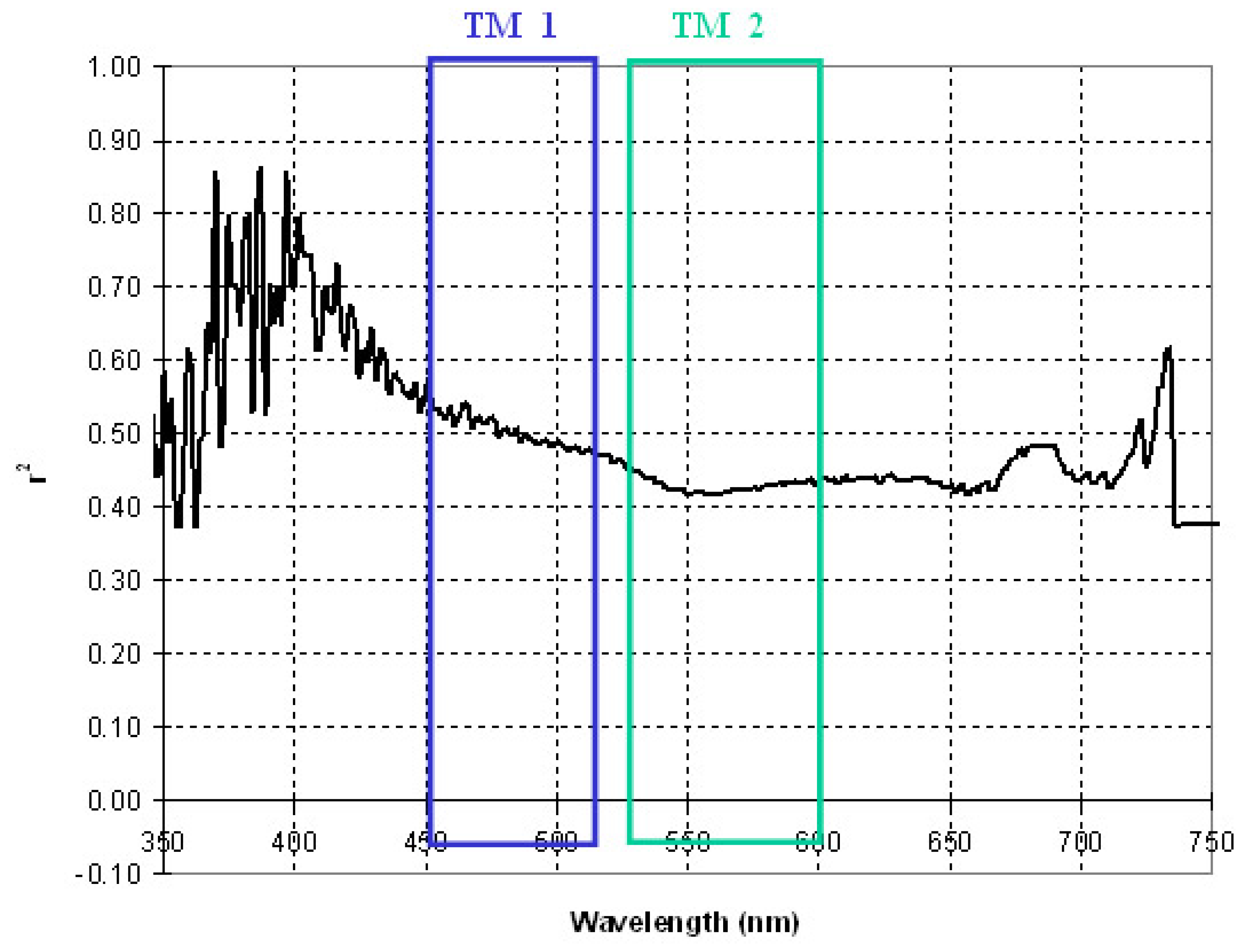
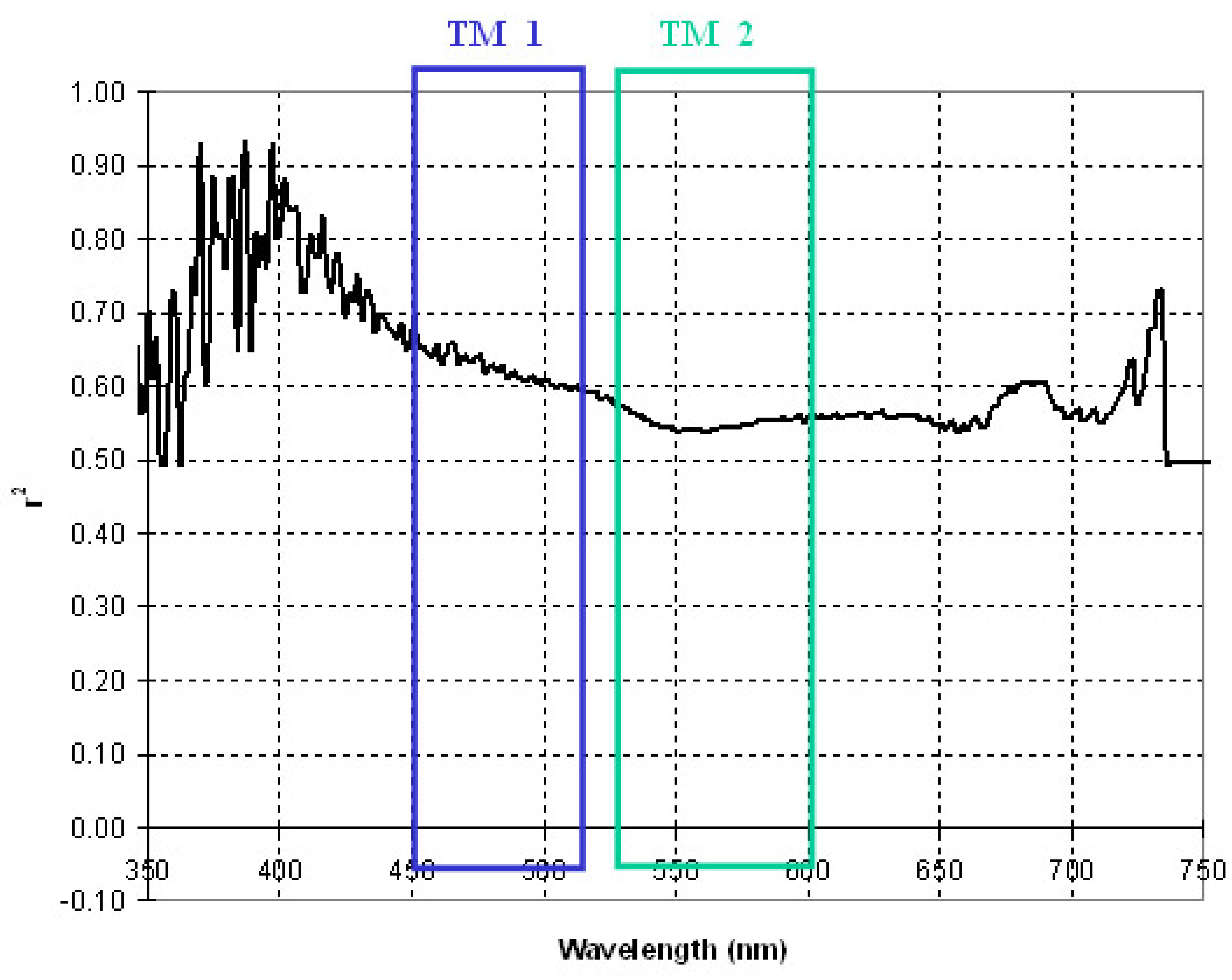
for chlorophyll-a, 400–450 nm (with r² 0.80–0.60) and 730–735 (with r² ≅ 0.60)

◆

for POC, 400–530 nm (with r² 0.80–0.60) and 728–735 (with r² ≅ 0.60).

Figure 4. Correlation expressed as r² between chlorophyll-a concentration and GER1500 reflectance for Datchet, Wraysbury and Queen Mary reservoirs (23 September 1998). Each r² value was calculated at each wavelength of the GER1500.

Figure 4. Correlation expressed as r² between chlorophyll-a concentration and GER1500 reflectance for Datchet, Wraysbury and Queen Mary reservoirs (23 September 1998). Each r² value was calculated at each wavelength of the GER1500.

Figure 5. Correlation expressed as r² between POC concentration and GER1500 reflectance for Datchet, Wraysbury and Queen Mary reservoirs (23 September 1998). Each r² value was calculated at each wavelength of the GER1500.

Figure 5. Correlation expressed as r² between POC concentration and GER1500 reflectance for Datchet, Wraysbury and Queen Mary reservoirs (23 September 1998). Each r² value was calculated at each wavelength of the GER1500.

From the findings shown above, it can be concluded that possible Landsat TM spectral regions for chlorophyll-a is TM band 1 and for POC are TM bands 1 and 2.

The GER 1500 experimental data was filtered through the RSR functions and averaged within the limits of the first four TM/ETM+ bands, to yield the in-band reflectance values. In order to retrieve the statistical relationship between the water quality parameters (e.g., Chl-a and POC) and the in-band reflectance measured from the GER1500, regression models have been applied and the outcomes are Equations 3 and 4.

Then, by applying the darkest pixel atmospheric correction [25] to a series of Landsat TM satellite images acquired on 5 March 1985, 4 July 1985, 8 October 1985, 13 February 1986 that were available during the water sampling of Chl-a and POC, several linear and multiple linear regression models were applied. The highest correlations (r² = 0.835) with the observed significance levels for F_observed and regression coefficients less than 0.005 were the following:

chl-a = 394.89 TM1 − 2.26

(3)

where

• chl-a: Chlorophyll-a concentration in μg/L
• TM1 is the reflectance from Landsat-5 TM1 (after atmospheric correction)

For POC, the predictive equation with the highest correlation (after atmospheric correction r²=0.782 and before correction r² = 0.024) was the following:

POC = 29,924.83 TM2 +146.57

(4)

where

• POC: Particulate organic carbon concentration in μg/L
• TM1 is the reflectance from Landsat-5 TM1 (after atmospheric correction)

Using the above Equations 3 and 4, an attempt was made to apply the darkest pixel atmospheric correction to other archived Landsat TM/ETM+ images acquired on 31 December 2001, 6 April 2002, 13 September 2002, 07 April 2000, 12 May 2001, 22 December 2001, 28 March 2002, 07 November 2002, 10 May 2006, 2 November 2006, 20 October 2007, 20 September 2008, 22 June 2010. The concentrations in Chl-a, the range was 0.57 to 4.20 μg/L and for the POC the range was 367 to 2,000 μg/L. The greatest Chl-a values corresponded to winter period in which there was no re-circulation and mixing of water in the reservoirs. The retrieved concentrations Chl-a and POC were complied with some available water quality measurements acquired from the boat water sampling for 2001, 2002 and 2006 periods. Based on these direct comparisons between the ‘modeled’ values found after applying Equations 3 and 4 with the in situ Chl-a and POC measurements, correlation coefficients of 0.9 and 0.92 were found.

4. Conclusions

For reaching the first objective in situ, reflectance spectra (i.e., 512 bands) have been used to identify optimal spectral regions from which Chl-a and POC can be retrieved. These spectral radiance measurements were transformed into relative percent reflectance and then resampled to correspond with the band configurations of the Landsat TM sensor that had been used for water quality assessment and monitoring. Linear regression analysis was applied to these transformed spectra in order to identify which spectral bands were the most useful (i.e., optimal) for retrieving of water quality in the Lower Thames Valley reservoirs in West London. This research identified the following optimal Landsat TM bands in the visible wavelength region:

▪

for chlorophyll-a, TM band 1 (0.45–0.52 µm)

▪

for POC, TM bands 1 (0.45–0.52 µm) and 2 (0.52–0.60 µm).

For retrieving the surface reflectance, which was the second objective of this study, a new method has been developed based on the use of the basic light attenuation equation and employment of fiber-optic probe and field spectro-radiometer.

By applying the darkest pixel atmospheric correction to a series of Landsat TM images acquired in 1985, two regression models were developed with correlation coefficients of 0.835 and 0.782 for Chl-a and POC cases. This was the third objective completed.

For further testing of the developed regression models, 12 Landsat TM/ETM+ band-1 images acquired in 2001 to 2010 were used to retrieve the Chl-a concentrations using only image-based data after atmospheric correction.

The developed regression models for Chl-a and POc using Landsat TM bands 1 and 2 can be further tested for possible transferability to other studies of water treatment reservoirs in the case where water optical characteristics and spectral signatures are considered the same.

The results have illustrated the potential of the blue and green band models to estimate chl-a and POC concentration in water treatment reservoirs from satellite data. However, challenges still remain in broadly applying the models to estimate absolute measures of chl-a and POC concentrations. With consideration for the effects of temporal variations of the concentrations of optically active constituents and the within-pixel spatial heterogeneity of the water body, it might be possible to have a better assessment of the accuracy of the blue and green band models. The application of atmospheric correction in any water quality monitoring study using satellite remote sensing is essential prior to any post-processing of image data.

Based on the fact that Landsat TM-5 and TM-7 are facing several problems; Landsat TM-5 is a very old sensor, its radiometric accuracy is compromised and, it will very likely end its life shortly; Landsat ETM+ has severe acquisition problems, several lines of each swath are systematically replaced by simulated values. However, the suitability and availability of such images are still useful in the remote sensing community. Moreover, there are not plans to replace these sensors in the forthcoming period. Indeed, other sensors such as ASTER, MODIS and MERIS have been widely used for water quality assessment studies and there is a great need, for every specific region in which remote sensing monitoring scheme is needed, to identify the spectral bands in which water quality parameters will be monitored. Indeed, such spectro-radiometric measurements and methods are essential to identify the suitable spectral region in which each water quality parameter could be retrieved so as to avoid errors or discrepancies during the application of correlation of satellite remotely sensed data and water quality parameters.

Despite the relatively low spectral and radiometric resolution of Landsat TM image data, the revisit capability and relatively low price per area make such satellite images useful for water quality assessment. The advances of using suitable imaging cameras for systematic monitoring can be assisted from the study in which field spectroscopy can be an ideal tool for identifying the suitable spectral region in which Chl-a or POC can be retrieved.

References

- Tyler, J.E.; Smith, R.C. In situ spectroscopy in ocean and lake waters. J. Opt. Soc. Am. 1965, 55, 800–805. [Google Scholar] [CrossRef]
- Tyler, J.E.; Smith, R.C. Spectro-radiometric characteristics of natural light under water. J. Opt. Soc. Am. 1967, 57, 595–601. [Google Scholar] [CrossRef]
- Blanchard, B.J.; Leamer, R.W. Spectral reflectance of water containing suspended sediment. In Proceedings of Symposium on Remote Sensing and Water Resources Management, Urbana, IL, USA, 11–14 June 1973; pp. 339–347.
- Jupp, D.L.B.; Kirk, J.T.; Harris, G.P. Detection, identification and mapping of cyanobacteria—Using remote sensing to measure the optical quality of turbid inland waters. Aust. J. Mar. Fresh Res. 1994, 45, 801–828. [Google Scholar] [CrossRef]
- Arenz, R.F. Reflectance and Absorption Spectrometry of Colorado Front Range Reservoirs. M.A. Thesis, Department of Environmental, Population, and Organismic Biology, University of Colorado, Population, Boulder, CO, USA, 1994. [Google Scholar]
- Arenz, R.F.; Lewis, W.M.; Saunders, J.F. Determination of chlorophyll and dissolved organic carbon from reflectance data for Colorado reservoirs. Int. J. Remote Sens. 1996, 17, 1547–1566. [Google Scholar] [CrossRef]
- Koponen, S.; Pulliainen, J.; Kallio, K.; Hallikainen, M. Lake water quality classification with airborne hyperspectral spectrometer and simulated MERIS data. Remote Sens. Environ. 2002, 79, 51–59. [Google Scholar] [CrossRef]
- Kallio, K.; Koponen, S.; Pulliainen, J. Feasibility of airborne imaging spectrometry for lake monitoring—A case study of spatial chlorophyll a distribution in two meso-eutrophic lakes. Int. J. Remote Sens. 2003, 24, 3771–3790. [Google Scholar] [CrossRef]
- Kallio, K.; Kutser, T.; Hannonen, T.; Kutser, T.; Koponen, S.; Pulliainen, J.; Vepsäläinen, J.; Pyhälahti, T. Retrieval of water quality variables from airborne spectrometry of various lake types in different seasons. Sci. Total Environ. 2001, 268, 59–77. [Google Scholar] [CrossRef]
- Hadjimitsis, D.G.; Clayton, C.R.I. Assessment of temporal variations of water quality in inland water bodies using atmospheric corrected remotely sensed image data. Environ. Monit. Assess. 2009, 159, 281–292. [Google Scholar] [CrossRef] [PubMed]
- Hadjimitsis, D.G.; Clayton, C.R.I.; Toulios, L. A new method for assessing the trophic state of large dams in Cyprus using satellite remotely sensed data. Water Environ. J. 2010, 24, 200–207. [Google Scholar] [CrossRef]
- Hadjimitsis, D.G.; Hadjimitsis, M.G.; Toulios, L.; Clayton, C.R.I. Use of space technology for assisting water quality assessment and monitoring of inland water bodies. Phys. Chem. Earth 2010, 35, 115–120. [Google Scholar] [CrossRef]
- Ramsey, E.W.; Jensen, J.R.; Mackey, H.; Gladden, J. Remote Sensing of water quality in active to inactive cooling water reservoirs. Int. J. Remote Sens. 1992, 11, 979–998. [Google Scholar] [CrossRef]
- Dekker, A.G. Detection of Optical Water Quality Parameters for Eutrophic Waters by High Resolution Remote Sensing. Ph.D. Thesis, Institute of Earth Sciences, Vrije Universiteit, Amsterdam, The Netherlands, 1993. [Google Scholar]
- Dekker, A.G.; Malthus, T.J.; Hoogenboom, H.J. The remote sensing of inland water quality. In Advances in Environmental Remote Sensing; Danson, F.M., Plummer, S.E., Eds.; John Wiley & Sons: Chichester, UK, 1995; pp. 123–142. [Google Scholar]
- Verdin, J.P. Monitoring water quality conditions in a large western reservoir with Landsat imagery. Photogramm. Eng. Remote Sens. 1985, 51, 343–353. [Google Scholar]
- Dewidar, K.; Khedr, A. Water quality assessment with simultaneous Landsat-5 TM at Manzala Lagoon Egypt. Hydrobiologia 2001, 457, 49–58. [Google Scholar] [CrossRef]
- He, W.; Chen, S.; Liu, X.; Chen, J. Water quality monitoring in a slightly-polluted inland water body through remote sensing—Case study of the Guanting Reservoir in Beijing, China, Front. Environ. Sci. Eng. 2008, 2, 163–171. [Google Scholar]
- Härmä, P.; Vepsäläinen, J.; Hannonen, T.; Pyhälahti, T.; Kämäri, J.; Kallio, K.; Eloheimo, K.; Koponen, S. Detection of water quality using simulated satellite data and semi-empirical algorithms in Finland. Sci. Total Environ. 2001, 268, 107–121. [Google Scholar] [CrossRef]
- Chen, Q.; Zhang, Y.; Hallikainen, M. Water quality monitoring using remote sensing in support of the EU water framework directive (WFD): A case study in the Gulf of Finland. Environ. Monit. Assess. 2007, 12, 157–166. [Google Scholar] [CrossRef] [PubMed]
- Pozdnyakov, D.; Shuchman, R.; Korosov, A.; Hatt, C. Operational algorithm for the retrieval of water quality in the Great Lakes. Remote Sens. Environ. 2005, 97, 352–370. [Google Scholar] [CrossRef]
- Hadjimitsis, D.G.; Hadjimitsis, M.G.; Clayton, C.R.I.; Clarke, B. Monitoring turbidity in Kourris Dam in Cyprus utilizing Landsat TM remotely sensed data. Water Resour. Manage. 2006, 20, 449–465. [Google Scholar] [CrossRef]
- Ormeci, C.; Sertel, E.; Sarikaya, O.O. Determination of chlorophyll-a amount in Golden Horn, Istanbul, Turkey using IKONOS and in situ data. Environ. Monit. Assess. 2008, 155, 83–90. [Google Scholar] [CrossRef] [PubMed]
- Becker, B.; Lusch, D.; Qi, J. Identifying optimal spectral bands from in situ measurements of Great Lakes coastal wetlands using second-derivative analysis. Remote Sens. Environ. 2005, 97, 238–248. [Google Scholar] [CrossRef]
- Hadjimitsis, D.G.; Clayton, C.R.I.; Hope, V.S. An assessment of the effectiveness of atmospheric correction algorithms through the remote sensing of some reservoirs. Int. J. Remote Sens. 2004, 25, 3651–3674. [Google Scholar] [CrossRef]
- Hadjimitsis, D.G. The Application of Atmospheric Correction Algorithms in the Satellite Remote Sensing of Reservoirs. Ph.D. Thesis, University of Surrey, School of Engineering in the Environment, Department of Civil Engineering, Guildford, UK, 1999. [Google Scholar]
- Milton, E.J. Principles of field spectroscopy. Int. J. Remote Sens. 1987, 8, 1807–1827. [Google Scholar] [CrossRef]
- Mccloy, K.R. Resource Management Information Systems; Taylor and Francis: London, UK, 1995; pp. 244–281. [Google Scholar]
- Milton, E.J.; Emery, D.R.; Kerr, C.H. NERC Equipment pool for field spectroscopy: Preparing for the 21st century. In Proceedings of the 23rd Annual Conference of the Remote Sensing Society, Observations & Interactions, Nottingham, UK, 1997; pp. 159–164.
- Milton, E.J.; Lawless, K.P.; Roberts, A.; Franklin, S.E. The effect of unresolved scene elements on the spectral response of calibration targets: An example. Can. J. Remote Sens. 1997, 23, 252–256. [Google Scholar] [CrossRef]
- Bukata, R.P.; Jerome, J.H.; Kondratyev, K.Y.; Pozdnyakov, D.V. Optical Properties and Remote Sensing of Inland and Coastal Water; CRS Press: Boca Raton, FL, USA, 1995. [Google Scholar]
- Markham, B.L.; Barker, J.L. Spectral characterisation of the Landsat Thematic Mapper sensors. Int. J. Remote Sens. 1985, 6, 697–716. [Google Scholar] [CrossRef]
- Wilson, A.K. The critical dependence of remote sensing on sensor calibration and atmosphere transparency. In Proceedings of the NERC 1987 Airborne Campaign Workshop, Swindon, UK, 15 December 1988; pp. 29–58.
- Li, Y.; Migliaccio, K. Water Quality Concepts, Sampling, and Analyses; CRC Press: Boca Raton, FL, USA, 2010. [Google Scholar]
- Tassan, S. An algorithm for the identification of benhtic algae in the Venice lagoon from Thematic Mapper data. Int. J. Remote Sens. 1992, 13, 2887–2909. [Google Scholar] [CrossRef]
- Gitelson, A.; Garbuzov, G.; Szilagy, F.; Mittenzwey, K.H.; Kranielli, A.; Kaiser, A. Quantitative remote sensing methods for real-time monitoring of inland water quality. Int. J. Remote Sens. 1993, 14, 1269–1295. [Google Scholar] [CrossRef]
© 2011 by the authors; licensee MDPI, Basel, Switzerland. This article is an open access article distributed under the terms and conditions of the Creative Commons Attribution license (http://creativecommons.org/licenses/by/3.0/).
Share and Cite
Hadjimitsis, D.G.; Clayton, C. Field Spectroscopy for Assisting Water Quality Monitoring and Assessment in Water Treatment Reservoirs Using Atmospheric Corrected Satellite Remotely Sensed Imagery. Remote Sens. 2011, 3, 362-377. https://doi.org/10.3390/rs3020362
Hadjimitsis DG, Clayton C. Field Spectroscopy for Assisting Water Quality Monitoring and Assessment in Water Treatment Reservoirs Using Atmospheric Corrected Satellite Remotely Sensed Imagery. Remote Sensing. 2011; 3(2):362-377. https://doi.org/10.3390/rs3020362
Chicago/Turabian StyleHadjimitsis, Diofantos G., and Chris Clayton. 2011. "Field Spectroscopy for Assisting Water Quality Monitoring and Assessment in Water Treatment Reservoirs Using Atmospheric Corrected Satellite Remotely Sensed Imagery" Remote Sensing 3, no. 2: 362-377. https://doi.org/10.3390/rs3020362