Article

Improved Feature Detection in Fused Intensity-Range Images with Complex SIFT (ℂSIFT)

Institute of Photogrammetry and Remote Sensing, Karlsruhe Institute of Technology, Kaiserstr. 12, D-76128 Karlsruhe, Germany
*
Author to whom correspondence should be addressed.
Remote Sens. 2011, 3(9), 2076-2088; https://doi.org/10.3390/rs3092076
Submission received: 1 July 2011 / Revised: 28 July 2011 / Accepted: 23 August 2011 / Published: 16 September 2011
(This article belongs to the Special Issue Terrestrial Laser Scanning)

Abstract

:
The real and imaginary parts are proposed as an alternative to the usual Polar representation of complex-valued images. It is proven that the transformation from Polar to Cartesian representation contributes to decreased mutual information, and hence to greater distinctiveness. The Complex Scale-Invariant Feature Transform (ℂSIFT) detects distinctive features in complex-valued images. An evaluation method for estimating the uniformity of feature distributions in complex-valued images derived from intensity-range images is proposed. In order to experimentally evaluate the proposed methodology on intensity-range images, three different kinds of active sensing systems were used: Range Imaging, Laser Scanning, and Structured Light Projection devices (PMD CamCube 2.0, Z+F IMAGER 5003, Microsoft Kinect).

1. Introduction

The detection of local features in data is of general interest in several disciplines, e.g., Photogrammetry, Remote Sensing, and Computer Vision. According to [1], good features should have the following properties: repeatability, distinctiveness/informativeness, locality, quantity, accuracy, and efficiency. A general overview of the performance of some important algorithms and resulting descriptors at points of interest is given by [2]. If points of interest are detected they can be utilised to locate correspondences between images. Various applications are known that are based on such points of interest, e.g., image-based registration, object recognition and segmentation, image stitching, self localisation, egomotion and trajectory estimation, as well as 3D reconstruction.
Typically, image-based registration methods focus on intensity images, which gives rise to the question of how to treat combined intensity-range data that can be obtained from particular sensors. For instance, existing registration methods for such data use either the intensity information or the range information, which is treated either as a point cloud, e.g., by applying the costly Iterative Closest Point (ICP) algorithm [3], or as an image, e.g., by applying the Scale-Invariant Feature Transform (SIFT) [4,5].
One might suggest that a separate treatment of the intensity and range data might be a sufficiently combined method. Indeed, some authors use the classical SIFT on range and intensity images separately [6,7,8,9,10]. This combined concept can in fact be viewed as representing the data with complex numbers which are close to the nature of the data itself: range measurements are often in fact phase measurements and intensity is obtained by measuring the amplitude. A possible dependence between range and intensity due to significant mutual information cannot be excluded. Depending on the application, greater mutual information can be desirable [11]. However, in feature detection low mutual information is important, and also fulfills the requirement “Distinctiveness/informativeness: The intensity patterns underlying the detected features should show a lot of variation, such that features can be distinguished and matched.”, as outlined by [1]. Therefore, considering the other traditional representation of complex numbers by the real and imaginary parts becomes important for fused intensity-range images. The fusion of intensity-range data asks for their holistic treatment. In the case of the Polar or Cartesian representation of such images, the Complex Scale-Invariant Feature Transform (ℂSIFT) is a natural generalisation of SIFT. Any particular interest detector, e.g., SURF, MSER, Harris, can be generalised to complex-valued images, SIFT has been chosen for reasons of example only.
Traditionally, the data consist of radiometric images captured with a passive sensor, e.g., a digital camera. Most active sensors, e.g., range imaging, laser scanning, or structured light projection devices provide additional intensity information beside the range. The measured intensity of active sensors can generally be separated in an active and passive intensity. The active intensity is often described as an amplitude and depends just on the measured scattering received by the active illumination with the sensor, e.g., a laser or diode. The passive intensity measured with an active sensor is often called background illumination, and depends on the illumination given by available extraneous light, e.g., sun light. The passive illumination captured with an active sensor might usually have low spectral information, due to the spectral bandpass filters which are in general used. Further, the range is measured which is for most users of main interest. Sometimes only a phase measurement is utilised to determine the range, where a limited uniqueness range is given by the lowest modulation frequency. These data can be described in a unified manner using complex numbers. This has the advantage of providing a general framework for passive and active sensors, without restrictions.
The aim of this article is to provide a method for obtaining in complex-valued images more independent real-valued representations by transformations which decrease mutual information. At the same time the method is aimed at increasing the number of features as well as the uniformity of their distribution.

2. Methodology

The complex-valued image description is introduced. Different representations of complex-valued images are compared with respect to mutual information. An evaluation method for estimating the uniformity of feature distributions is proposed.

2.1. Complex-Valued Image Description

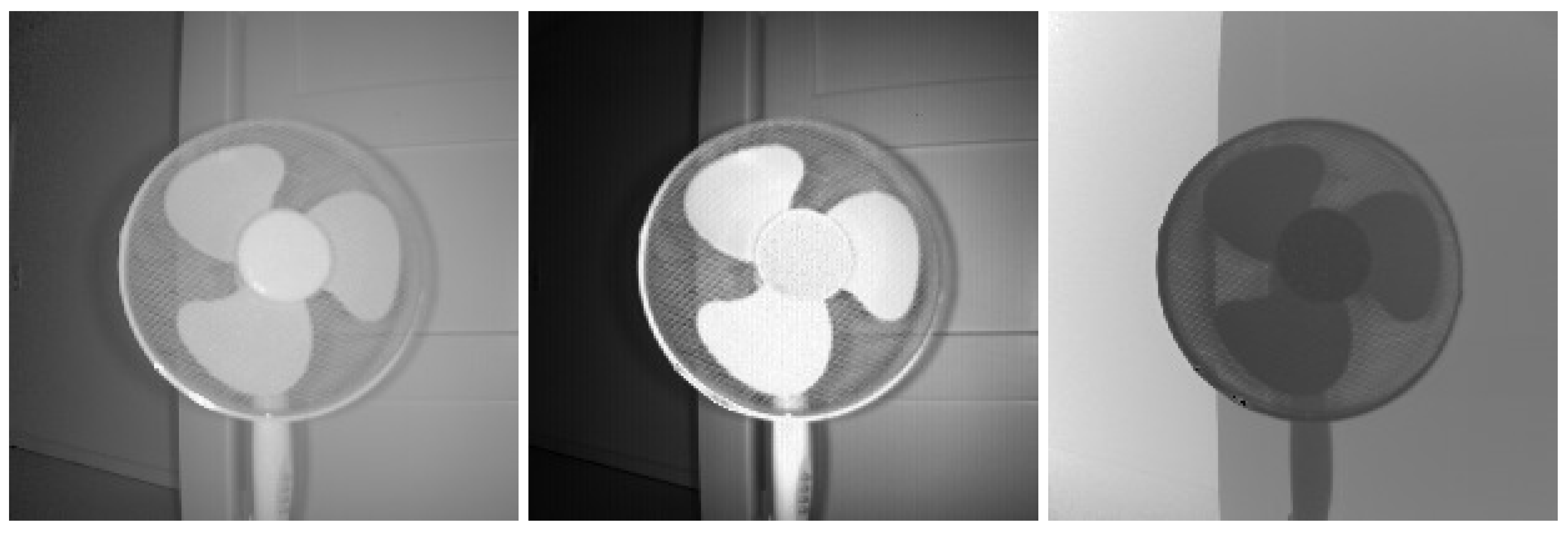
The data provided by active sensors consists of the active and passive intensities together with the range information. In this article, it is assumed that the latter is given by a phase measurement. In this wide-spread method, the phase is usually interpreted as actual distance. However, this approach causes problems if the observed object is at a distance beyond the uniqueness range. For this reason, we will always interpret that information as what it is: namely a phase value (Note: The measured phase difference (a physical quantity) can be represented by a phase value (a mathematical quantity).). Hence, a description of an active-passive image using complex numbers becomes quite natural.
Throughout this article, x , y are image coordinates, r = r ( x , y ) is the range image, I a ( x , y , r ) the active intensity image, and I p ( x , y ) the passive intensity image. The latter does not depend on the range r. The complex-valued image function is now defined as:
f ( x , y , r ) = I p ( x , y ) + I a ( x , y , r ) e i ϕ ( x , y , r ( x , y ) )
where the phase ϕ = ϕ ( x , y , r ) [ 0 , 2 π ) is defined via the range
r = n · 2 π + ϕ
with n N . Notice that passive intensity is treated here as an offset. In this setting, 2 π is the uniqueness range of the camera with N . The natural number is a multiple of some unit of length, and n is the “wrapping number”.
The two standard ways of representing complex numbers yield two different image representations: the Polar representation
f = f e i   arg ( f )
where
f = I p 2 + 2 I p I a cos ϕ + I a 2
arg ( f ) = arctan I a sin ϕ I p + I a cos ϕ
and the Cartesian representation
f = Re ( f ) + i Im ( f )
where
Re ( f ) = I p + I a cos ϕ
Im ( f ) = I a sin ϕ
Throughout the article, it is assumed that
max f = 1
for all complex images. This normalisation can be achieved through division by the maximal value of f . The remainder of this article will discuss these two different representations of complex images coming from different types of sensors from the entropy perspective.

2.2. Mutual Information in Complex-Valued Images

If a representation of complex-valued images f with real values is given, the image-value dimension is at least two. However, the information content of data is known to depend on their representation. For complex-valued images, this means that some real-valued representations could be more preferred than others from the viewpoint of information theory. For this purpose, the differential entropy is defined as
E q = R ρ ( q ) log ρ ( q ) d q
where R is the range of quantity q, d q is a probability measure and ρ ( q ) is the distribution function of q.
If q = ( A , ω ) , then E q = E A , ω becomes the joint entropy of amplitude A = f and phase ω = arg ( f ) . Likewise, E X , Y is the joint entropy of the real and imaginary parts X = Re ( f ) , Y = Im ( f ) of the complex-valued image:
f = A cos ω + i A sin ω
It is a fact that the entropy of a system depends on the choice of coordinates, the change in entropy being dependent on the Jacobian of the transformation (cf. e.g., [12]). In the case of complex-valued images, this general result specialises to a preference of Cartesian over Polar coordinates:
Theorem 2.1. 
The transformation from the Polar to the Cartesian image representation increases the entropy. More precisely, it holds true that
E A , ω = E X , Y + log A
where
log A = ρ ( X , Y ) log A ( X , Y ) d X d Y < 0
and ρ ( X , Y ) is the joint distribution function of X = Re ( f ) and Y = Im ( f ) .
Proof. 
The statement follows from the well-known transformation rule of the distribution function:
ρ ( X , Y ) = ρ ( A , ω ) · J
where J is the Jacobian of ( A , ω ) ( X , Y ) , the transformation from the Polar to the Cartesian image representation. In this case, J = A ( X , Y ) = X 2 + Y 2 1 , since A is normalised amplitude by Equation (9). It follows that the mean log A is negative.                ☐
As a consequence, Theorem 2.1 allows to compute the difference in mutual information
MI ( a , b ) = E a + E b E a , b
for the pairs ( X , Y ) and ( A , ω ) from the individual entropies:
μ : = MI ( X , Y ) MI ( A , ω ) = ( E X + E Y ) ( E A + E ω ) + log A
and the quantity μ becomes a measure for the gain of independence by transforming from Polar to Cartesian image representation. Namely, MI ( a , b ) = 0 if and only if the quantities a and b are independent, and MI ( a , b ) can be interpreted as the degree of dependence between a and b. This allows to formulate:
Conjecture 2.2. 
For almost all complex-valued images, there is a gain of independence by transforming from the Polar to the Cartesian image representation. In other words: μ < 0 for almost all complex-valued images.
In fact, the experiments of Section 3 indicate that
E X + E Y E A + E ω
which means that log A 0 .

2.3. Naive Approach

For range measurements within the uniqueness range, the well-known inverse-square law of active intensity implies the approximation:
I a I p ϕ 2
where the phase φ is identified with the range r (w.l.o.g. = 1 in Equation (2)). This means that it does make sense to consider I a and I p as correlated and detect features only in the pair ( I a , ϕ ) . This is called the naive approach. Hence, there are two successive transformations leading to our complex image in Polar representation:
I a e i ϕ f e i arg ( f ) Re ( f ) + i Im ( f )
where
f 2 = I a 2 ϕ 4 + 2 ϕ 2 cos ϕ + 1
arg ( f ) = arctan sin ϕ ϕ 2 + cos ϕ
Re ( f ) = I a ( ϕ 2 + cos ϕ )
Im ( f ) = I a sin ϕ
with Jacobian of the composite map being
J = I a ϕ 2 cos ϕ 2 ϕ sin ϕ + 1
We wish to exclude the possibility that the benefit from log f 0 of the second transformation (Polar to Cartesian image representation with Jacobian J = f ) is jeopardised by the first transformation with Jacobian J .
The relation between J , J and J for general composed transformations ( a , b ) ( a , b ) ( a , b ) is known to be
J = J · J
Hence,
E a , b = E a , b + log J + log J
and it follows that
log J = log J + log J
where the means are each taken over the corresponding probability distribution. Hence, we would like to exclude large positive values of log J . From Equation (20), Equation (24) and Equation (25), it follows that
J = ϕ 2 cos ϕ 2 ϕ sin ϕ + 1 ϕ 4 + 2 ϕ 2 cos ϕ + 1
which depends only on φ. Notice that the denominator is strictly positive, and a closer look reveals that log J < 0 if φ is not concentrated in some specific small neighbourhood of π.
Notice, that the inverse-square law in Equation (18) can be used to estimate missing values of I a or I p in order to obtain our complex image representation. Use of this will be made in the following section.

2.4. Feature Distribution in Complex-Valued Images

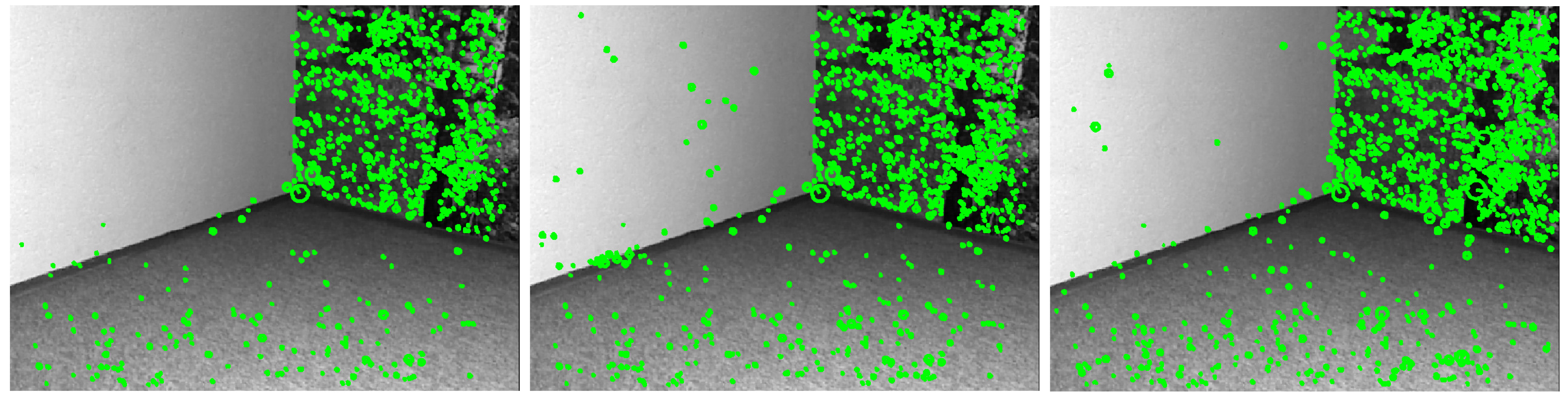
Scale-space feature detection usually involves finding extrema in real-valued functions, and these are obtained from the image through filtering. In the case of complex-valued images f, it makes sense to detect features individually in the components of a representation over the real numbers. This means, for the Polar representation, the detection of features in f and in arg ( f ) , and for the Cartesian representation in Re ( f ) and Im ( f ) . The classical SIFT can be applied to any kind of real-valued images. In particular, applying SIFT to the pairs ( f , arg ( f ) ) or ( Re ( f ) , Im ( f ) ) componentwise defines ℂSIFT. If the complex-valued image is represented by the pair ( u , v ) of real values, a feature for ℂSIFT is defined as a point which is a classical SIFT-feature for u or v.
The preferred representation usually has the desired property that it contains more features, and these are also more uniformly distributed over the image grid than in other representations. More texture in an image can be obtained by increasing the entropy. Hence, a transformation whose Jacobian has absolute value less than one yields more texture by Equation (14), and Theorem 2.1 then says that the Cartesian representation yields more structure than the Polar representation. On the other hand, using the scale-space equation t f = Δ f aims at finding texture which is sufficiently persistent through the filtering cascade. Hence, increasing entropy of the image derivative leads to more persistent texture. And also from this persistence point of view, the Cartesian representation turns out more advantageous than the Polar representation:
Theorem 2.3. 
Transforming from Polar to Cartesian image representation increases the entropy of the scale-space derivatives:
E A ˙ , ω ˙ = E X ˙ , Y ˙ + A · cos ω ˙ sin ω sin ω ˙ cos ω
with
A · cos ω ˙ sin ω sin ω ˙ cos ω < 0
where the expectation value is taken over the joint probability distribution of X ˙ and Y ˙ .
Proof. 
In the light of Theorem 2.1, the statement follows from the Jacobian
J = A · cos ω ˙ sin ω sin ω ˙ cos ω
of the transformation of derivatives.                ☐
A Cartesian feature in a complex-valued image is defined to be a scale-space feature for Re ( f ) or Im ( f ) , and, similarly, a Polar feature of f is a scale-space feature for f or arg ( f ) . Consequently, one can formulate:
Conjecture 2.4. 
The expected number of Cartesian features is larger than the expected number of Polar features for almost all complex-valued images f.
It is natural that a mere increase in the number of features is not sufficient for many applications, e.g., the more the points of interest are concentrated in one small portion of the image, the less relevant their number becomes for estimating the relative camera pose. Hence, an important issue is the distribution of features on the image grid. In fact, it is often desired to know that they are sampled from a uniform distribution.
For n independent, identically distributed random variables X i , the empirical distribution function F n ( x ) is defined as
F n ( x ) = 1 n i = 1 n δ ( , x ] ( X i )
where δ ( , x ] is the indicator function
δ ( , x ] ( Y ) = 1 , Y x 0 otherwise
Then, by the Glivenko-Cantelli Theorem [13,14], the F n converge uniformly to their common cumulative distribution function F:
F n F = sup x R F n ( x ) F ( x ) 0 a . s .
with increasing number n of observations. For arbitrary cumulative distribution functions F, the expression F n F is known as the Kolmogorov-Smirnov statistic. It has the general properties of a distance between cumulative distribution functions. Therefore, it will be called here the KS-distance.
In the case of a snapshot taken from a scene, one can assume that the observed n features are produced by the scene independently from another. By viewing the scene as the single source of features, one can further assume that the features are identically distributed. In other words, they can be assumed taken from a common cumulative distribution function F.
However, there seems to be no straightforward generalisation of the KS-distance to the multivariate case, as indicated by [15], in particular the proposed generalisations seem to lack robustness. Therefore, we simply propose the Euclidean norm of the two coordinate-wise KS-distances:
d ( S , λ ) : = F n x λ x 2 + F n y λ y 2
where S is a sample of n points in the plane, F n i is the empirical distribution function, λ i and λ are the cumulative density functions of the uniform distribution on the i-coordinate axis and on the plane, respectively. This will be called the Euclidean KS-distance to uniformity. Conjecturally, there will be more uniformity in the detected scale-space features for the Cartesian representation than in those for the Polar representation. Let S Cartesian be the sample of Cartesian features, and S Polar the sample of Polar features of a given complex-valued image f. Then:
Conjecture 2.5. 
For almost all complex images f, the transformation from Cartesian to Polar image decreases the Euclidean KS-distance to uniformity:
d ( S Cartesian , λ ) < d ( S Polar , λ )
where λ is the uniform distribution on the image plane.
Conjecture 2.2 says that the pair S Re ( f ) , S Im ( f ) will be more independent than S f , S arg ( f ) . Conjecture 2.4 says that there will be more Cartesian than Polar features. Intuitively, these conjectures together support Conjecture 2.5.

3. Experiments

In order to experimentally evaluate the proposed methodology, three different kinds of active sensing systems were used to capture data from three different scenes: Range Imaging (RIM), Terrestrial Laser Scanning (TLS), and Structured Light Projection (SLP) devices.

3.1. Range Imaging (RIM)

The PMD [Vision] CamCube 2.0 captures range and intensity simultaneously. The former is obtained through phase measurements, and the latter is differentiated between active and passive intensity. The measured active intensity depends on the illumination by the sensor, whereas the passive intensity depends on the background illumination (e.g., the sun or other light sources). The uniqueness range of 7.5 m is defined by the utilized modulation frequency of 20 MHz.
The data meet exactly the requirements of the methodology. The image size for all data is 204 × 204 pixels. Figure 1 shows the values of I p , I a , and φ, respectively.
Figure 1. RIM. I p , I a , φ (from left to right).
Remotesensing 03 02076 g001

3.2. Terrestrial Laser Scanning (TLS)

The Z+F IMAGER 5003 is a standard phase-based laser scanner with survey-grade accuracy within the mm range. While scanning the scene a phase is measured and by using the modulation frequency the range between scanner and object surface is calculated. Again the uniqueness range of 79 m is given by the lowest utilized modulation frequency. Also measured is the intensity I raw which is a mixture of active and passive intensity, because the different intensities are not distinguished.
To adapt the measured data to the methodology, the range image is converted to a phase image φ, and the intensity is separated to active and passive intensity using the inverse-square law in Equation (18). The indoor scene in Figure 2 guarantees that all range values lie within the uniqueness range. The selected image area has 532 × 468 pixels. The I raw and φ are shown.
Figure 2. TLS. Left: I raw , Right: φ.
Remotesensing 03 02076 g002

3.3. Structured Light Projection (SLP)

In Microsoft’s Kinect for the Xbox 360, active range measurement is based on continuously-projected infrared structured light. Additionally an RGB image is synchronously captured. Due to the multi-static sensor design where the sensors are at different locations, the data are captured with a slight parallax. Through a calibration, the images are properly aligned.
Finally, in order to adapt the measured data to the methodology, the measured range image is interpreted as a phase image with uniqueness range given by the measured maximal range value. The RGB image, after conversion to gray values, is interpreted as the passive intensity image I p . In the same way as with the TLS data, Equation (18) is used to estimate I a . The images have 480 × 640 pixels. Figure 3 shows I p and φ.
Figure 3. SLP. Left: I p , right: φ.
Remotesensing 03 02076 g003

4. Results

Table 1 shows the entropy results for the various images. A first observation is that the real parts Re ( f ) have similar entropies as the absolute values f and are relatively high, whereas the entropies of the imaginary parts Im ( f ) are relatively low and similar to those of the angle values arg ( f ) . The last two columns show firstly that the main contribution to the gain of independence μ comes from the Jacobian of the transformation. Secondly, there is an extra gain due to the observed validity of inequality (17). In all examples, the Cartesian images are more independent than the Polar images.
Table 1. Entropy, mean log-Jacobian, and mutual information.
PolarCartesian
E I raw E f E arg ( f ) E Re ( f ) E Im ( f ) log f μ
RIM7.41846.67611.09767.07631.29910.94941.2929
TLS7.22827.2134.91656.67634.64841.21931.4772
SLP7.81067.19251.05437.25950.98790.83030.8309
For the feature detection with ℂSIFT, Vedaldi’s Matlab implementation of SIFT [16] was used. ℂSIFT was applied on two snapshots of the same scene. A pair of homologous matched feature points is given by a successful ℂSIFT matching of candidate keypoints at most one pixel apart. Table 2 reveals that complex images contain more homologous matched feature points than the sole intensity image, and the Cartesian representation contains more than the Polar representation.
Table 2. Number of homologous matched feature points.
I raw f arg ( f ) Polar Re ( f ) Im ( f ) Cartesian
RIM15915959218156119275
TLS13351335222155756711331700
SLP1004100481108596710842051
Table 3 indicates that the complex feature points are more uniformly distributed than those in the corresponding intensity image. In all examples, the Cartesian representation has the smallest Euclidean KS-distance to uniformity. Figure 4 depicts the locations of the homologous matched feature points in the SLP case. It can be observed that the raw intensity has no valid detections in the left sector consisting of a homogeneous surface. Both complex image representations have more texture in that sector, therefore valid features are detected. The Polar image contains a cluster in the left border between the left and the bottom sector which is likely responsible for the relatively large horizontal KS-distance to uniformity. The right sector has a large amount of texture in all cases. However, in contrast to the others, the Cartesian image contains valid features very near the right boundary of that sector.
Table 3. KS-distances to uniformity of homologous matched feature points.
horizontalverticalEuclidean
S raw S Polar S Cartesian S raw S Polar S Cartesian S raw S Polar S Cartesian
RIM0.182940.170350.164020.124870.111940.127450.221490.20390.20754
TLS0.16990.180240.18150.173690.161880.155850.242970.242640.23921
SLP0.048550.0642630.0598430.0513290.0334110.0365080.0706520.0724290.0701
Figure 4. Homologous matched feature points in SLP image: S raw , S Polar , S Cartesian (from left to right).
Remotesensing 03 02076 g004

5. Conclusions

High mutual information of variables a, b means that they are redundant. Therefore, it is of interest to compare the two standard representations of complex-valued images: the Polar and the Cartesian representation. We have deduced through theoretical considerations the general conjecture that the mutual information of the real and imaginary parts of an information is lower than the amplitude and phase parts. We have verified this experimentally by applying ℂSIFT, and have found that not only does the number of valid detected features increase through transforming from the Polar to the Cartesian image representation, but also the uniformity of their distribution.
The implication is that in feature detection within fused intensity-range images, as e.g., obtained by Range Imaging, Laser Scanning or Structured Light Projection devices, the Cartesian representation is to be preferred over the Polar representation in order to achieve more distinctiveness and informativeness, one of the requirements for local features from [1].

Acknowledgments

The authors would like to thank Sven Wursthorn and Martin Weinmann for fruitful discussions.

References

  1. Tuytelaars, T.; Mikolajczyk, K. Local invariant feature detectors: A survey. Found. Trends Comput. Graph. Vis. 2008, 3, 177–280. [Google Scholar] [CrossRef] [Green Version]
  2. Mikolajczyk, K.; Schmid, C. A performance evaluation of local descriptors. IEEE Trans. Pattern Anal. Mach. Intell. 2005, 10, 1615–1630. [Google Scholar] [CrossRef] [PubMed]
  3. Rusinkiewicz, S.; Levoy, M. Efficient Variants of the ICP Algorithm. In Proceedings of the 3rd International Conference on 3D Digital Imaging and Modeling (3DIM), Quebec City, QC, Canada, 28 May–1 June 2001; pp. 145–152.
  4. Lowe, D. Object Recognition from Local Scale-Invariant Features. In Proceedings of the International Conference on Computer Vision (ICCV 1999), Corfu, Greece, 20–23 September 1999; pp. 1150–1157.
  5. Lowe, D. Distinctive image features from scale-invariant keypoints. Int. J. Comput. Vis. 2004, 60, 91C110. [Google Scholar] [CrossRef]
  6. Haker, M.; Böhme, M.; Martinetz, T.; Barth, E. Scale-Invariant Range Features for Time-of-Flight Camera Applications. In Proceedings of IEEE Computer Society Conference on Computer Vision and Pattern Recognition Workshops, CVPRW08, Anchorage, AK, USA, 23–28 June 2008.
  7. Barnea, S.; Filin, S. Keypoint based autonomous registration of terrestrial laser point-clouds. ISPRS J. Photogramm. Remote Sens. 2008, 63, 19–35. [Google Scholar] [CrossRef]
  8. Böhm, J.; Becker, S. Automatic Marker-Free Registration of Terrestrial Laser Scans Using Reflectance Features. In Proceedings of the 8th Conference on Optical 3D measurment Techniques, Zurich, Switzerland, 9–12 July 2007; pp. 338–344.
  9. Wang, Z.; Brenner, C. Point Based Registration of Terrestrial Laser Data Using Intensity and Geometry Features. In Proceedings of the International Archives of the Photogrammetry, Remote Sensing and Spatial Information Science, Beijing, China, 3–11 July 2008; Volume XXXVII, pp. 583–590.
  10. Weinmann, M.; Weinmann, M.; Hinz, S.; Jutzi, B. Fast and automatic image-based registration of TLS data. ISPRS J. Photogramm. Remote Sens. 2011, in press. [Google Scholar] [CrossRef]
  11. Sawada, H.; Mukai, R.; Araki, S.; Makino, S. Polar coordinate based nonlinear function for frequency-domain blind source separation. IEICE Trans. Fundam. Electron. Commun. Comput. Sci. 2003, E86-A, 590–596. [Google Scholar]
  12. Hnizdo, V.; Gilson, M. Thermodynamic and differential entropy under a change of variables. Entropy 2010, 12, 578–590. [Google Scholar] [CrossRef] [PubMed]
  13. Glivenko, V. Sulla determinazione empirica della legge di probabilita. Giorn. Ist. Ital. Attuari 1933, 4, 92–99. [Google Scholar]
  14. Cantelli, F. Sulla determinazione empirica della legge di probabilita. Giorn. Ist. Ital. Attuari 1933, 4, 221–424. [Google Scholar]
  15. Lopes, R.; Reid, I.; Hobson, P. The Two-Dimensional Kolmogorov-Smirnov Test. In Proceedings of the XI International Workshop on Advanced Computing and Analysis in Physics Research, Amsterdam, The Netherlands, 23–27 April 2007.
  16. Vedaldi, A. SIFT for Matlab. Available online: http://www.vlfeat.org/∼vedaldi/code/sift.html (accessed on 1 September 2011).

