Retrieval of Coarse-Resolution Leaf Area Index over the Republic of Kazakhstan Using NOAA AVHRR Satellite Data and Ground Measurements

1
Department of Geography, Geogr-August University Göttingen, Goldschmidtstr. 5, D-37077 Göttingen, Germany
2
Institute of Bioclimatology, Georg-August University Göttingen, Büsgenweg 2, D-37077 Göttingen, Germany
*
Author to whom correspondence should be addressed.
Remote Sens. 2012, 4(1), 220-246; https://doi.org/10.3390/rs4010220
Submission received: 1 November 2011
/
Revised: 28 December 2011
/
Accepted: 28 December 2011
/
Published: 13 January 2012
Abstract
:A new multi-decade national-wide coarse-resolution data set of leaf area index (LAI) over the Republic of Kazakhstan has been developed based on data from the Advanced Very High Resolution Radiometer (AVHRR) and in situ measurements of vegetation structure. The Kazakhstan-wide LAI product has been retrieved using an algorithm based on a physical radiative transfer model establishing a relationship between LAI and given patterns of surface reflectance, view-illumination conditions and optical properties of vegetation at the per-pixel scale. The results revealed high consistencies between the produced AVHRR LAI data set and ground truth information and the 30-m resolution Landsat ETM+ LAI estimated using the similar algorithm. Differences in LAI between the AVHRR-based product and the Landsat ETM+-based product are lower than 0.4 LAI units in terms of RMSE. The produced Kazakhstan-wide LAI was also compared with the global 8-km AVHRR LAI (LAI_PAL_BU_V3) and 1-km MODIS LAI (MOD15A2 LAI) products. Results show remarkable consistency of the spatial distribution and temporal dynamics between the new LAI product and both examined global LAI products. However, the results also revealed several discrepancies in LAI estimates when comparing the global and the Kazakhstan-wide products. The discrepancies in LAI estimates were outlined and discussed.
1. Introduction
Leaf area index (LAI), defined as the one-side area of leaves per unit of ground area [1], is one of the key biophysical variables needed for the modeling of energy balance, evapo-transpiration, photosynthesis, and carbon sequestration. Ground-based estimations of LAI are based either on direct contact or indirect optical methods [2,3]. Ground-based measurements can provide excellent accuracy of LAI estimations. The main disadvantages of ground-based LAI estimations are that they are (1) time- and work-consuming and (2) can provide values only for site-specific or stand-specific targets. However, for various biophysical models over large areas, broad-wide estimations of LAI at regional to global scales are needed. For such estimations, application of remote sensing-based approaches is the most attractive possibility.
Over the years, efforts to improve upon the quality of LAI estimates using remote sensing have resulted in the adoption of a variety of different approaches. The most used approach for scaling-up of ground-measured LAI to large areas bases on empirical models relating LAI to surface reflectance and to spectral vegetation indices (SVI) derived from reflectance values. There is a large number of SVI applied for mapping LAI from remotely sensed data. Among the most applied SVI are the Normalized Difference Vegetation Index (NDVI), the Simple Ratio (SR) [4,5]. However, recent studies showed that these indices can provide good-accuracy results only in canopies with relatively low LAI values and small background reflectance [6]. For areas with high background reflectance or high biomass values such as forests, the Reduced Simple Ratio (RSR) and the Corrected Normalized Difference Vegetation Index (NDVIc), which incorporate additional information from the short-infrared bands, are reported to have stronger response to LAI [7–9]. However, empirical models based on the relationships between LAI and SVI are site-, time- and biome-specific [7,10]. From these reasons, their use may be effective only at the scales from local to regional.
Another widely used approach for scaling-up LAI bases on the use of physical models. This approach has gained particular importance for estimation of the global products of LAI with a coarse spatial resolution (1-km and more). In physical models, retrieval of LAI is based on inversion of three-dimensional radiative transfer problem. Commonly, the algorithm of radiative transfer models employs the look-up-table method using a number of biome-specific constants related to canopy architecture, soil and vegetation optical properties [11,12].
A number of global LAI products are being routinely estimated using data of spatial moderate and coarse-resolution from various satellite sensors such as Moderate Resolution Imaging Spectroradiometer (MODIS), Systeme Pour l’Observation de la Terre (SPOT) VEGETATION, and Medium Resolution Imaging Spectrometer (MERIS). The global LAI products produced from MODIS, SPOT and MERIS data have a frequency of 1–2 weeks and cover timely a period of somewhat more than one decade [13–15]. For retrieval of the LAI data sets with a temporal cover of longer than one decade, the use of data from the Advanced Very High Resolution Radiometer (AVHRR) onboard NOAA 7–14 series of satellite platforms is the single possibility. A global LAI product on the base of AVHRR NDVI data in combination with a radiative transfer model has been already developed at the end of the 1990s [16]. Validation of this LAI product has shown promising results [17]. Research into producing a new global multi-decade leaf area index data set for the period 1981 to 2006 derived from AVHRR NDVI in combination with the MODIS LAI algorithm is currently being undertaken [18].
The above LAI products have been widely used for various biophysical models, operating at spatial scales from regional to global and temporal scales from an individual growing season to multi-year periods. However, the application of the global LAI products is hampered by several restrictions such as the lack of regional validation, spatial and temporal discontinuity due to cloud cover and instrument problems [19–21]. As a result, despite the fact that the quality of the LAI global products, especially that of the MODIS LAI product, is being regularly enhanced [18,21–23], several studies have developed either their own multi-year LAI data sets or modified the existing global LAI data sets for applications at the national to regional scale [9,24–26].
The Republic of Kazakhstan is the largest country in Central Asia and the ninth-largest country in the world (2.7 million km2). The grassland of Kazakhstan represents one of the world’s hugest carbon pools [27–29]. Evaluation of the existing global LAI products in Kazakhstan’s biomes and generation of new national and regional LAI products is of great importance with respect to the recent efforts towards mapping carbon sequestration in grasslands of Kazakhstan [30–32]. Unfortunately, the area of Kazakhstan has been out of scope of the validation efforts of the global LAI products undertaken by the international remote sensing community during last 10 years. A small number of new LAI data sets for Kazakhstan generated at the Institute of Geography of the University Göttingen [33–35] have somewhat narrowed the existing research gap but not closed it entirely.
In this paper, we describe a new spatial coarse-resolution national-wide LAI data set derived from 8-km resolution AVHRR NDVI data by implementing a three-dimensional radiative transfer model. To obtain better adaptation to real conditions, the developed model is calibrated using ground truth data for the precise description of canopy architecture through the determination of the site-specific canopy light extinction coefficient at the pixel level. The spatial accuracy of the product was evaluated using LAI assessed from spatial high-resolution Landsat ETM+ imagery and ground-based data. The spatial and temporal consistency was evaluated against the respective coarse resolution MODIS standard products (MOD15A2 LAI) and the global AVHRR LAI product (LAI_PAL_BU_V3). The national-wide AVHRR LAI product allows the prediction of more representative LAI values for the territory of Kazakhstan and provides the possibility to improve the global AVHRR LAI values in Kazakhstan regarding their validity.
2. Data
2.1. Ground-Based Leaf Area Index
2.1.1. Sampling Strategy for Ground-Based Measurements
In situ measurements of vegetation structure variables including LAI were undertaken during three field campaigns in June 2004, June 2008, and August 2008. The sampling strategy organized by plot and subplot was based on a stratified sampling. In this sampling strategy, we tried to include as much as possible vegetation types and their variations in the validation campaign. In situ measurements of vegetation structure parameters were carried out at 50 sampling plots established within the main vegetation types which cover the most part (99.2%) of Kazakhstan’s territory: grassland, cropland, shrubland, woodland, mixed forest, deciduous broadleaf forest, and deciduous needleaf forest. Establishing plots in each of the validation sites, we made efforts to locate our plots so that their location records all possible variations within the vegetation type caused by the terrain and soil conditions. Extensive analyses of topographic maps (scale 1:100,000) and fine-resolution satellite images (Landsat data) were undertaken in order to determine most favorable locations of sampling plots within each of the validation sites.
In all cases, the plot size for the in situ measurements was 90 × 90 m2 corresponding to an area observed by 3 × 3 Landsat ETM+ pixels [36]. The measurements were made in a 30-m transect raster spacing within each plot. Totally, 14 measurements were completed at subplots within each of the sampling plots which were than averaged to mean values over corresponding plots. The information about test sites, the measurements time, measurement methods, and measured values is listed in Table 1.
2.1.2. Computations of Leaf Area Index from Ground-Based Measurements
Direct contact destructive and indirect non-contact optical methods were used to acquire ground-based vegetation structure variables. The direct contact destructive method uses data from biomass harvesting to calculate LAI [2]. This method is time-consuming and expensive. However, the advantage of this method is a very high accuracy of LAI estimation. Often, results from direct LAI estimations serve as reference for estimations by indirect non-contact methods [1,2]. Among other approaches for LAI estimation, indirect non-contact optical methods are the most widely used during last two decades because of their effectiveness and low time- and cost-consumption [1–3]. These methods use hemispherical photography to obtain the canopy closure (vegetation cover fraction) which is a parameter strongly correlated with LAI. With regard to application in Kazakhstan, hemispherical photography was tested for LAI estimation in grassland and shrubland in recent studies [33,34]. These studies reported very good appropriateness of the optical methods for the use in these vegetation types.
In the field campaigns in 2008, hemispherical photos were made using a WinScanopy Image Acquisition instrument developed by REGENT INSTRUMENTS [37]. For the processing of hemispherical photographs and retrieval of vegetation structure variables we used the Can Eye software [38]. Gap fraction, the proportion of unobstructed sky, was calculated at 5° zenith angle intervals and used for additional calculations. LAI and other vegetation structure indices were calculated using routine procedures included in the Can Eye software. Calculating formulae and operation of Can Eye are described in detail in the Can Eye manuals following the methods described by [1,3]. The LAI is corrected for non-random distribution of foliage elements based on the clumping index, which is calculated using the logarithmic gap averaging technique given by [39].
For a number of plots measured in June 2004, the direct contact method was employed to obtain LAI. By this method, LAI was converted from harvested biomass by multiplying it by specific leaf area (SLA, projected leaf area per kg leaf carbon). Dry matter content was measured by drying samples of aboveground biomass (AGB) in an oven. The proportion of carbon in AGB was assumed to be 0.47 [40]. SLA was assumed to be a biome-dependent variable which standard values for individual biomes were taken from [41]. LAI was then estimated as:
The suitability of the direct contact approach for estimation of LAI was assessed by comparing the obtained LAI values with the LAI values computed from the hemispherical photography [33]. The results of this comparison revealed general associations between the indirect optical and direct contact measured LAI. For a deeper insight into the methodology and results of this comparison, please see the study by [33].
2.2. Satellite Data
2.2.1. Spatial Coarse-Resolution AVHRR Data
For this study we used the Global Inventory Modelling and Mapping Studies (GIMMS) NDVI data set compiled at 8-km spatial resolution from the NOAA AVHRR satellite data by the GIMMS research group [42] covering the period 1982 to 2008. The GIMMS NDVI data are freely distributed over the Internet as 30-day maximum value composites to minimize effects of cloud contamination [43]. Pre-processing includes minimization of noise resulting from residual atmospheric effects, orbital drift effects, inter-sensor variations, and stratospheric aerosol effects by a series of corrections, including temporal compositing, spatial compositing, orbital correction, calibration for sensor drifts, and atmospheric correction [42]. In order to remove some non-vegetated artifacts remaining in the GIMMS NDVI data set, we carried out an additional calibration of the data set against three invariant desert targets located in Taklimakan desert using a method described by [44].
2.2.2. High-Resolution Satellite Data
Four Landsat scenes covering the ground data collection sites at the time of the in situ measurements of LAI were downloaded from the Landsat archive [45]. The Landsat imagery was used to create high-resolution maps of LAI which were afterwards applied for validation of the coarse-resolution LAI product (see Section 4.5). The location and characteristics of each scene are listed in Table 2.
The Landsat scenes were pre-processed using the common steps of satellite image processing such as geometric and atmospheric corrections, and geo-referencing. The geo-referenced scenes were registered using ground control points obtained from 1:100,000 topographic maps. The registration was accurate to within ±1 pixel. Atmospheric corrections were made to convert the radiance measurements at the top of the atmosphere to the surface-level reflectance. The dark-object subtraction (DOS) method was adopted to account for contradicting effects of both path radiance and atmospheric transmittance. DOS approach bases on the assumption of the existence of dark objects (zero or small surface reflectance) throughout a Landsat scene and a horizontally homogeneous atmosphere [46]. The minimum reflectance value in the histogram from the entire scene is thus attributed to the effect of the atmosphere and is subtracted from all the pixels. For pre-processing of our Landsat data we used clear water as the dark object to derive atmospheric optical information for radiometric normalization. On this way, we determined a minimum reflectance value for each scene and subtracted it from all the pixels in the scene. The terrain slope and aspect effects on reflectance values have been addressed using topographic normalization methodology based on the non-lambertian Minnaert model [47]. This approach seeks to approximate bidirectional reflection characteristics by introducing empirically derived constants. The empirical constants for this correction were computed for each Landsat scene according to the non-lambertian reflection behavior of the surface.
2.2.3. Land Cover Data
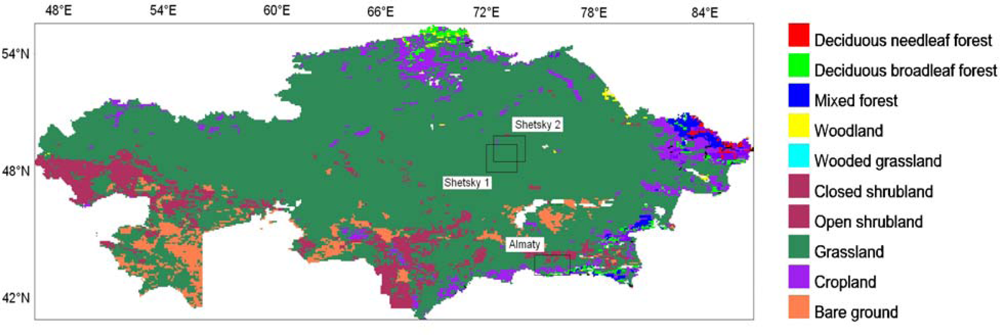
A land cover classification data set over the region was taken from the global land cover data derived from the 8-km spatial resolution AVHRR data by the Global Land Cover Facility group [48]. This data set is accessible in the Global Land Cover Facility archive centre [49]. There are 11 vegetation types in the study region (Figure 1). The largest area is covered by grassland (2.12 × 10⁶ km2), following by open shrubland (0.213 × 10⁶ km2) and cropland (0.157 × 10⁶ km2).
Using this land cover data in our study, we were aware that the map represents a distribution of the land cover classes corresponding to the period 1981–1994. As the study period spanned over 30 years, land cover parameters could be inconstant during the whole study period and may exhibit some alterations from decade to decade and even from year to year. However, with respect to our modeling approach, we suggested that such changes would not significantly affect our results. The reason is that most of the model’s input parameters are vegetation type-specific; the parameters are assigned as constants for four vegetation types: grass, shrubs, bushes, and woody vegetation. Bearing this in mind, our long-year experience in this region, recent published studies, and extensive discussions with country’s experts gave us evidences that most changes are associated with vegetation dynamics within a certain vegetation type; they do not lead to any transitions from one vegetation type to another (for instance: from forest to grassland or vice versa). This means that the spatial distribution of vegetation types remains more or less stable throughout the period of our study. For example, if any area of cropland has been abandoned and is undergoing a restoration process, this area belongs further to grass vegetation.
3. Methods
3.1. Radiative Transfer Model to Derive Satellite-Based LAI
A radiative transfer model based on an inverse method for solving the Beer-Lambert law, taking into account the effect of zenith angle on the extinction coefficient and clumping index, was employed to produce satellite-based LAI. The used model was explained in details by [26] so only a short illustration is provided here.
In the model LAI is defined as follows and has evolved from [50]:
where fC is fractional vegetation cover and k(θ) is the light extinction coefficient for a solar zenith angle θ.
3.2. Fractional Vegetation Cover
Fractional vegetation cover was estimated based on application of spectral mixture analysis (SMA) method to NDVI data. A simple SMA model assumes that the value of vegetation index of a given pixel is the proportion-weighted combination of the two-endmembers spectra (green vegetation and bare soil) [51,52]. Such a model interprets the NDVI value of a given pixel as the sum of contributions from canopy and background reflectance. SMA models have been widely used with various satellite data to produce time-series of fractional vegetation cover for use in numerical biogeochemistry models [53,54]. The formulation of a SMA can be based on a linear relationship between NDVI and fractional cover where fC is simply scaled between the lower and upper limits of bare soil and maximum NDVI [50]. Otherwise, a SMA model can assume a non-linear relationship between the variables [52,55].
For our purpose, we examined both linear and non-linear approaches between NDVI and fC and found that the following non-linear equation was most appropriate at the regional scale in Kazakhstan:
where v and s denote values of NDVI over fully vegetated area (fC = 1.0) and bare soil (fC = 0.0).
Determination of values used for NDVIs and NDVIv was based on the techniques thoroughly described in the recent literature [51–54]. Parameter NDVIs is typically 0.05 for all land covers and is considered not to vary much from year to year [53,54]. NDVIv was determined by means of a detailed analysis of the histogram of annual maximum NDVI for each vegetation cover category. The use of ground truth data on fC in our study has made the selection of NDVI value for completely vegetated areas in the histogram maximally objective.
3.3. Modelling Light Extinction Coefficient
The light extinction coefficient k for a solar zenith angle θ was calculated as a function the canopy projection factor (G), the clumping index (Ω) and cosines of the solar zenith angle θ using the equation from [56,57]:
The parameter G takes the value of 0.5 for all solar elevation angles, if the leaves are distributed uniformly over the surface of a sphere. Values of G for non-uniform leaf distribution for varying solar zenith angles were calculated using the equation from [58]:
In this equation, x is the ratio of vertical to horizontal projection of canopy elements. The value of x can be estimated using an empirical equation relating x to the canopy leaf inclination angle Θ [59]:
For spherical canopies Θ = 57.4°, for planophile canopies 0° < Θ < 57.4°, and for erectophile canopies 57.4° < Θ < 90°. For our purpose, average values of the canopy leaf inclination angle for individual vegetation types were retrieved from hemispherical photos by the Can Eye software.
The clumping factor a solar zenith angle θ was modeled using the equation from [59]:
where Ωmax is the maximum clumping index for a canopy, c is a canopy-specific coefficient to be defined, and p is a function of x, given as
3.4. Retrieval of 8-km Spatial Resolution Data Set of LAI for the Area of Kazakhstan
The national-wide 8-km AVHRR LAI product over the Republic of Kazakhstan for the period 1982–2008 was derived using the following steps:
- The fC model (Equation (3), Section 3.2) was applied to 1-month composite GIMMS NDVI images from 1982 through 2008. The input parameters NDVIs and NDVIv were obtained for each vegetation class respectively.
- Vegetation class-specific parameters x, Ωmax, c, and Θ for modeling the light extinction coefficient (Equations (4–8)) were determined. The average leaf inclination angle Θ for each individual vegetation class was modeled from hemispherical photos using the routine procedure included in the Can Eye software. After that, the ratio of vertical to horizontal projection of canopy elements x for individual vegetation types was calculated using Equation (6). The maximum clumping index for an individual vegetation type was assumed to be equal to the highest Ω among all test sites within this vegetation type. The parameter c for Equation (7) was obtained by inverting this equation for a known value of the clumping index which was retrieved from hemispherical photography.
- The algorithm for the light extinction coefficient was applied at the 8-km pixel scale using a combination of vegetation class-specific input parameters, the gridded data set of mean monthly solar zenith angle, the NOAA AVHRR Land Cover and GTOPO30 elevation data sets [60] to retrieve maps of the light extinction coefficient for the whole area of Kazakhstan. Temporally, the monthly maps of the extinction coefficient covered the period 1982–2010.
- LAI maps were estimated for each 1-month composite period from January 1982 through December 2008 employing the above LAI retrieval algorithm (Equation (2)) using the data sets produced by the processing steps 1 and 3.
3.5. Validation of the 8-km Spatial Resolution Kazakhstan-Wide AVHRR LAI Product
3.5.1. Comparison with Ground-Based Data
The new national-wide AVHRR LAI product was first validated directly with ground-measured LAI data over Kazakhstan. However, there are problems that we face when we try to compare spatial coarse-resolution products with ground measurements. Recent studies revealed that the direct comparison between ground measured parameters and coarse resolution satellite data cannot be efficient because the coarse pixel scale is much greater than a plot’s scale and results of such a comparison would be poor. Local variance of ground measurements is always much more than that at a coarse scale making a direct comparison problematic. Therefore, the up-to-date direct validation approach consists of using transfer functions and high-resolution imagery to scale up the ground measurements to the spatial resolution of the product [22,61]. In this approach, a spatial high-resolution map of the variable of interest is introduced. When aggregated to coarse resolution, this map serves as the ground-truth information.
In the presented study, the 8-km LAI product was compared with the LAI estimated from Landsat ETM+ imagery on the basis of regression analysis. Nevertheless, we should be aware that there are possible uncertainties that we face as we generalize the fine-resolution LAI map to 8-km spatial resolution blocks because most of the environmental processes are scale-dependent [62]. LAI is a highly variable local characteristic; through a spatial degradation to a coarse-resolution blocks LAI loses its spatial heterogeneity. However, the problem of scaling up data can be adequately treated using a geostatistical approach such as block kriging [62]. Block kriging can estimate a spatial variable over scales or domains larger than that of the original observations. In the present study, we used block kriging to re-scale data from the fine-resolution (30-m Landsat ETM+) to the coarse resolution (8-km AVHRR data).
For our purpose, we produced high-resolution maps of LAI using 30-m resolution Landsat imagery which were than aggregated to the 8-km resolution and compared with the AVHRR retrievals of the LAI product. Landsat-based estimations of LAI were generated using empirical models between the ground measurements and reflectance in Landsat bands as transfer functions. For validation of the coarse-resolution LAI retrievals for the years 2004 and 2008, we applied the available high-resolution LAI data sets which had been developed using empirical models in previous studies by the authors [33,34]. For direct validation of the AVHRR LAI at the Almaty test site for August 2008, we developed a new empirical model based on the relationship between the ground measurements of LAI in this year and the corresponding Landsat ETM+ image. These high spatial resolution LAI maps were degraded to 8-km spatial resolution of AVHRR data and compared using pixel-by-pixel approach with the corresponding AVHRR LAI values.
3.5.2. Comparison with Other LAI Products
Finally, the produced AVHRR LAI data set was suggested to compare with other independent satellite-based LAI data sets: (1) the MODIS collection 5 LAI product (MOD15A2) and (2) the global AVHRR LAI product (LAI_PAL_BU_V3). The MODIS LAI products (collection 5) are available for the public from the Earth Observing System Data Gateway [63]. Thorough description of MOD15A2 is given by [12,13]. The global AVHRR LAI product is available on-line at http://cybele.bu.edu/modismisr/products/avhrr/avhrrlaifpar.html. For a detailed description of LAI_PAL_BU_V3 see [16] and [18].
4. Results
4.1. The New National-Wide 8-km Spatial Resolution AVHRR LAI Data Set
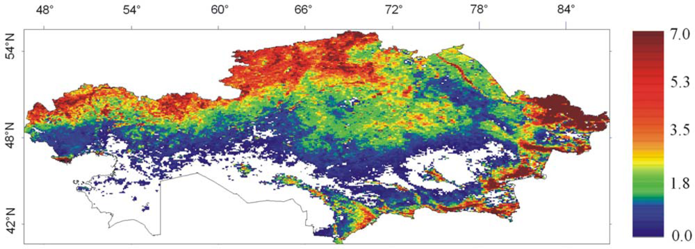
Figure 2 shows the modeled national-wide AVHRR LAI for June 2008. It demonstrates a large spatial LAI variability. The values of LAI vary from 0 in the south of Kazakhstan to more than 6 in the northern and north-eastern parts of Kazakhstan. The spatial distribution of LAI over the area of Kazakhstan generally reflects the pattern of vegetation classes in the republic (compare to Figure 1). Areas of bare soil and some areas of shrubland in the desert zone are characterized by zero values of LAI. Low values of LAI are observed in the shrubland of the desert/semi-desert zones in the southern and central parts of Kazakhstan. High values of LAI correspond to the forest zones, broadleaf and needleleaf forests, whereas especially high LAI values (>6) are observed in the needleleaf forests in the mountain regions located in the north-east and south-east parts of Kazakhstan.
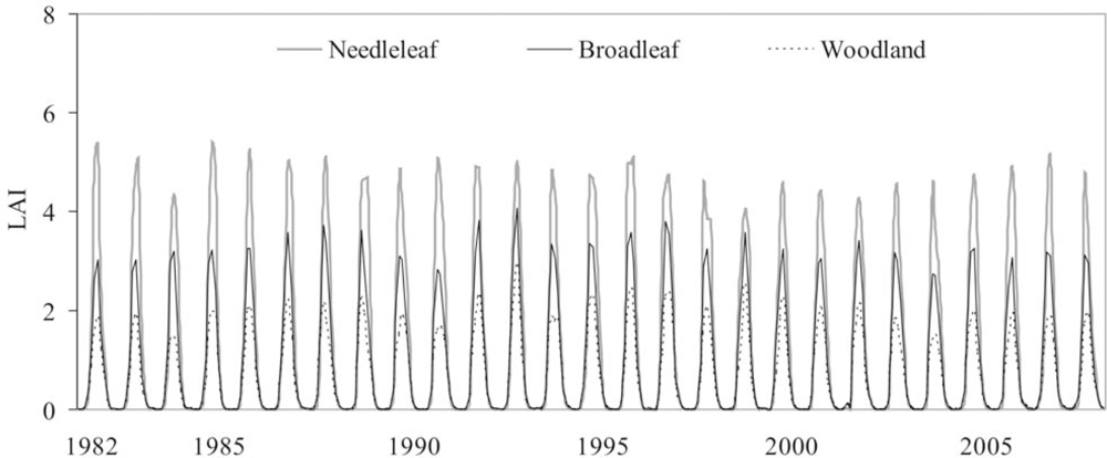
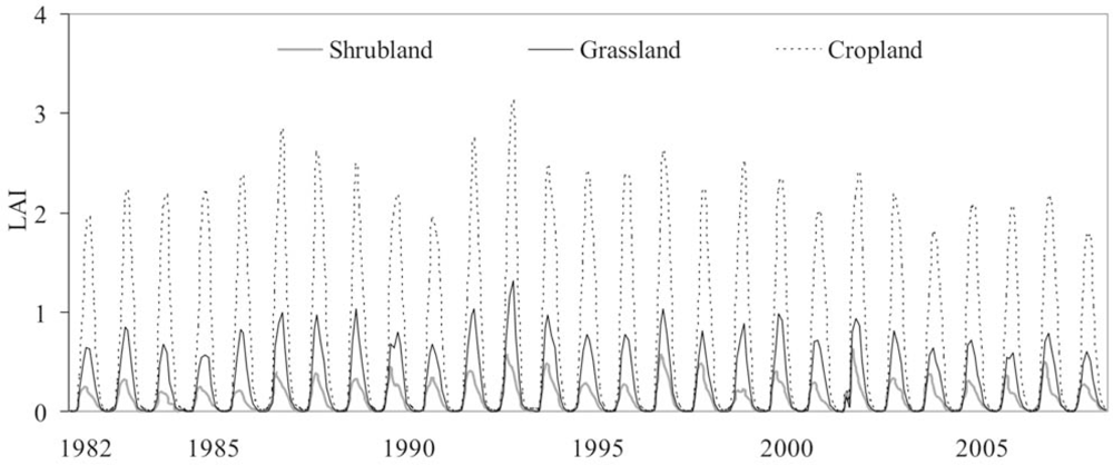
In Figure 3 the monthly courses of the LAI for the 6 main landcover classes (needleleaf forest, broadleaf forest, woodland, shrubland, grassland, and cropland) in Kazakhstan during the years 1982–2008 are plotted. The area-averaged LAI values were created for pixels with the same landcover class within the area of Kazakhstan. The LAI profiles demonstrate that the LAI product reproduces adequately the inter-annual and intra-annual variability of LAI. In all vegetation types, the plant growth starts up in March–April when air temperature rises above zero. In the shrubland, grassland, and cropland classes, the maximum LAI is commonly achieved in the late May–early June, whereas the forests and woody areas demonstrate the LAI peak in July (Figure 3) The LAI of the shrubland, grassland, and cropland decreases earlier than that of the forest classes, reflecting the earlier senescence of vegetation due to drought-like conditions caused by the decreased precipitation and high temperatures in July–August. Outside of the growing season, all the presented vegetation classes have generally a LAI value of zero.
4.2. Validation
4.2.1. Validation at the Grassland Site in Central Kazakhstan (Shetsky Region)
The fine-resolution RTM algorithm and the relationship between field measured LAI and empirically based models for the ETM+ images were used to produce 30-m maps of LAI for the whole Shetsky region. The fine-resolution algorithm differs from the algorithm used to generate the AVHRR LAI product in that uses fine-resolution inputs data sets corresponding to the ETM+ spatial resolution. This was run with the fC map derived from the corresponding ETM+ NDVI data. The LAI-NDVIc relationship derived from field measured LAI and ETM+ image was used to produce a regression-based 30-m LAI map for June 2004 [34], while Canonical Correlation Analysis Index was employed for June 2008 [33].
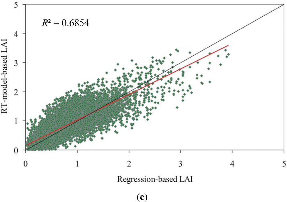
As first, we compared the results of the fine-resolution RTM LAI with field measurements. A good agreement between the Landsat ETM+ LAI and field measured LAI is observed for both validation years. Thus, for 2008 (Figure 4(a)), the fine-resolution RTM LAI explained 79% of spatial variation in ground based LAI (R2 = 0.79 and RMSE = 0.08). The relationship between modeled LAI and ground based LAI for 2004 is somewhat weaker but also sufficiently strong (R2 = 0.69 and RMSE = 0.13) (Figure 4(b)). Second, we carried out a pixel-by-pixel comparison of the 30-m spatial resolution LAI maps produced by the RTM algorithm and the regression-based algorithm (Figure 4(c)). The retrievals from both algorithms correlate strongly at the per-pixel scale (R2 = 0.69, RMSE = 0.22). These results demonstrate that the used RTM algorithm works effectively at the 30-m spatial resolution.
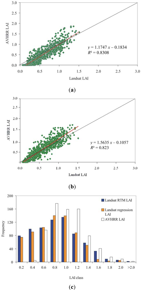
Next, we degraded the 30-m LAI maps to the spatial resolution of AVHRR using the block kriging-based re-scaling procedure [62]. After that, we compared the degraded maps with the coarse resolution LAI product over the Shetsky region. The AVHRR LAI shows strong correlation at the pixel level both with the RTM-retrieved and regression-retrieved Landsat LAI products (Figure 5): R2 = 0.83 and RMSE = 0.20 for the RTM-retrieved LAI, compared to R2 = 0.82 and RMSE = 0.22 for the regression-derived Landsat LAI. The slope of the regression line was 1.17 for the comparison of the RTM-based Landsat LAI (Figure 5(a)) and 1.36 for the regression-based Landsat LAI. These small slope values mean that the AVHRR LAI somewhat overestimates high values and underestimates low values of the ETM+ LAI. However, in both cases, the regression line falls very close to the 1:1 line, indicating that the compared LAI products are very similar.
Finally, we examined the frequency distribution of the LAI modeled using 30-m Landsat (both RTM and regression-based algorithms) and 8-km AVHRR data (Figure 5(c)). The histograms reveal that the LAI distribution of the AVHRR data sets is generally consistent with that of the Landsat data sets. However, the AVHRR LAI histogram shows a slight trend to higher values in comparison to the Landsat histograms, while the LAI classes at the left range are not occupied. As anticipated, the coursing of the spatial resolution by modeling LAI increases general homogeneity of the area occupied by a pixel. The increased homogeneity exposes then a lower spatial variation of the LAI variable [9,22]. On the other hand, the results of the comparisons illustrate that a sufficient amount of the information on spatial distribution of LAI is retrievable by coarse spatial resolution AVHRR imagery; even though a quantity of information is lost in comparison to the Landsat ETM+ results.
4.2.2. Validation at the Almaty Wood/Forest Site
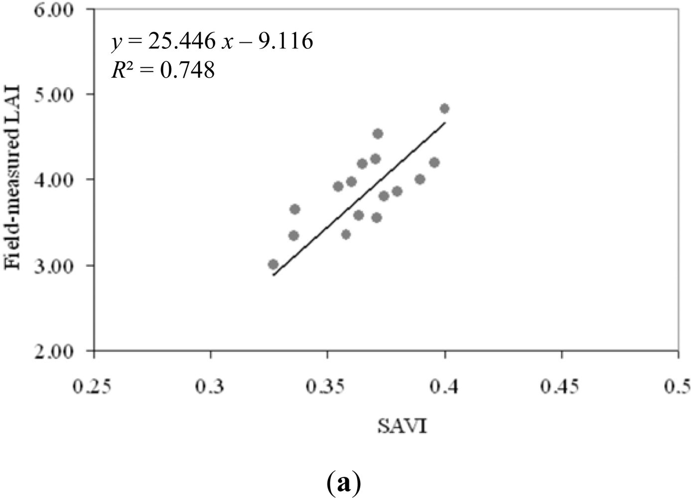
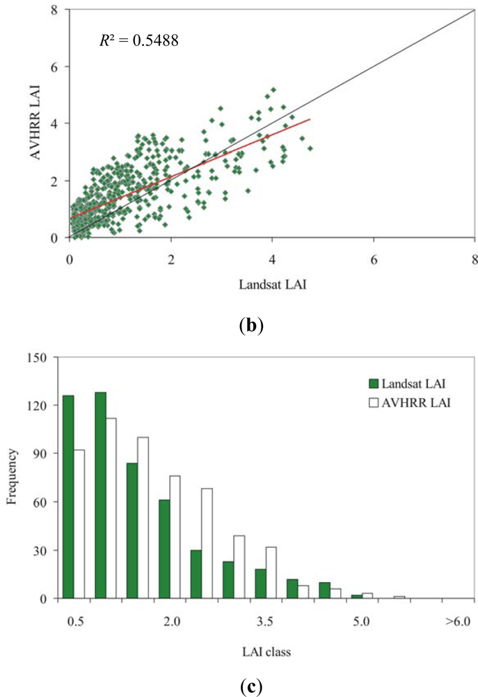
A Landsat ETM+ image acquired on 30 July 2009 was used to generate the fine-resolution LAI map for validation procedure. 30-m maps of LAI produced by the RTM algorithm is suggested to compare with the produced AVHRR LAI data at the Almaty wood/forest site. In order to obtain the model with the best prediction power, we tested several vegetation indices such as the Simple Ratio (SR), the Normalized Difference Vegetation Index (NDVI), the Reduced Simple Ratio (RSR), and the Soil Adjusted Vegetation Index (SAVI) [64]. The SR and NDVI were found to be not suitable for the generation of fine-resolution LAI map because of high amount of understory vegetation in the test forest site. The SAVI and the shortwave infrared incorporating index RSR showed high correlation with the ground measured LAI. However, the best correlation with field measurements was obtained by using the SAVI as predictor (Figure 6(a)). The regression model was selected to generate the fine-resolution LAI map over the wood/forest area in the region of Almaty (R² = 0.75, RMSE = 0.38). The map was re-projected to geographic latitude/longitude system and degraded to 8-km resolution using the block kriging-re-sampling procedure. Using the NOAA AVHRR land cover map, areas covered by woodland and forest were extracted from the LAI map and used for further comparison with the AVHRR LAI product. Figure 6(b) shows the pixel-by-pixel comparison between the AVHRR LAI and the reference Landsat LAI values. The AVHRR LAI explains 55% of the spatial variance in the Landsat LAI. Histograms in Figure 6(c) demonstrate some discrepancies in the LAI frequency obtained from the Landsat and AVHRR data sets. Thus, the AVHRR LAI has lower frequency in the left- and right-range classes (0.5 < LAI < 1.5, and LAI > 4.0), while the middle-range classes (1.5 < LAI < 4.0) are characterized by considerable higher frequency. Nonetheless, the comparison shows that differences between Landsat LAI and AVHRR LAI are lower than 0.5 LAI in terms of RMSE fulfilling the general accuracy requirement for LAI estimates from multiple sensors.
4.3 Comparison with LAI_PAL_BU_V3 Monthly Composite LAI Data
4.3.1. Spatial Consistency of the Data Sets
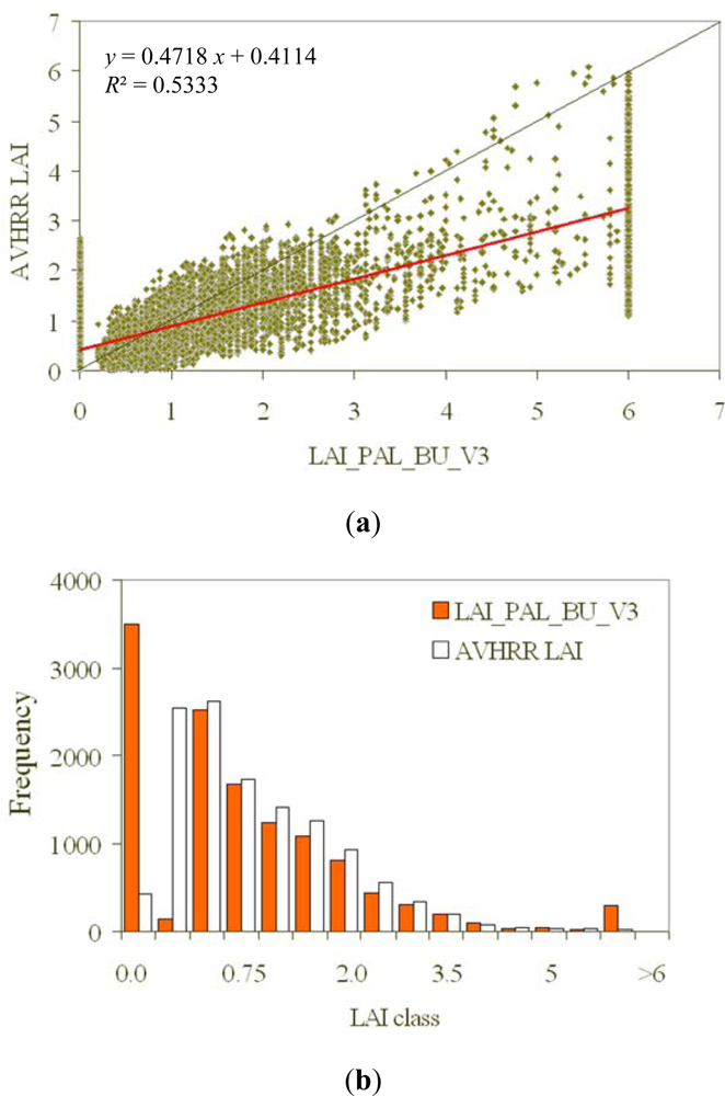
The comparison of AVHRR LAI and LAI_PAL_BU_V3 for July 2008 indicates a significant consistency with an overall performance about 0.65 in terms of RMSE, despite of a relatively high scattering around the regression line (Figure 7(a)). The comparison reveals that LAI_PAL_BU_V3 values exceed the AVHRR LAI values for the greatest part of pixels. However, sometimes, the AVHRR LAI is greater, especially for LAI ranges of 1 to 3. In the other months of 2008, pictures are similar. These discrepancies are partially due to different algorithm specifications, and differences in auxiliary data, particularly land cover map. In comparison to the LAI_PAL_BU_V3 values, the estimated AVHRR LAI show stronger variations in spatial and temporal dimensions, especially in the areas with very low and very high vegetation density. Thus, LAI_PAL_BU_V3 product has significantly shorter value variety, the values range from 0.12 to 6.0, while values of the AVHRR product range from 0 to more than 6.0. The LAI = 6 threshold determines the possible highest value in LAI_PAL_BU_V3 product. This threshold is associated with the highest possible vegetation density and is employed to the forest areas with closed vegetation canopy [16]. Pixels with the vegetation fractional cover less than 0.2 have LAI = 0 assuming generally no green vegetation in such areas [16]. However, for similar pixels, the AVHRR LAI product calculates LAI values greater than 0 assuming the presence of green vegetation in these areas despite of the very infrequent vegetation cover. For areas with very high vegetation density, the LAI_PAL_BU_V3 algorithm signs a LAI value of 6.0 neglecting both spatial and temporal variability. On contrary, the AVHRR LAI reproduces the variability of LAI between pixels within such areas. The discrepancies in the prediction of the LAI range values are also reflected in the histograms (Figure 7(b)). The histogram produced from the AVHRR LAI shows the classic random distribution with a right skewenness, whereas in the LAI_PAL_BU_V3 distribution the range LAI classes (0–0.2 and 5.5–6.0) have too high frequency exposing the non-random distribution.
The slope of AVHRR LAI versus LAI_PAL_BU_V3 was significantly lower than the 1:1 line suggesting that the LAI_PAL_BU_V3 algorithm overestimates LAI values. The overestimation of LAI values by the LAI_PAL_BU_V3 product also has impact on the predicted mean value. The spatially averaged LAI in July is 1.52 for the AVHRR LAI versus 1.85 for the LAI_PAL_BU_V3 estimation.
4.3.2. Temporal Consistency of the Data Sets
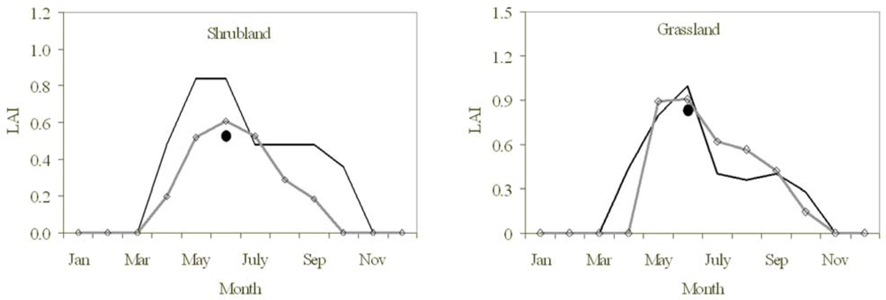
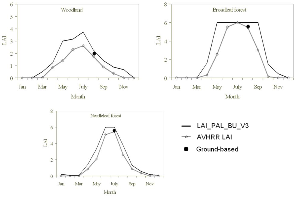
To compare the main features of the temporal behavior of the coarse-resolution LAI products, the 30-day LAI time series for a single year are drawn in Figure 8 for the major vegetation classes—shrubland, grassland, woodland, broadleaf forest and needleleaf forest, forest types—over the test areas. In Kazakhstan and other countries of Central Asia, the vegetation variability is generally associated with intra-annual seasonality of green leaf area. Among the shown biomes, only needleleaf forest shows high-consistent dynamics between the Kazakhstan-wide AVHRR LAI and LAI_PAL_BU_V3 LAI. For other shown biomes, there are some differences in capturing the seasonal dynamics of leaf production by the data sets. The profiles derived from the LAI_PAL_BU_V3 product are generally characterized by significantly higher LAI values throughout the growing season. In all cases, the LAI estimations provided by the Kazakhstan-wide AVHRR LAI product were closer to the ground-based LAI values than that by the LAI_PAL_BU_V3 product. For shrubland, grassland, woodland and broadleaf forest, the LAI estimates provided by the LAI_PAL_BU_V3 product are also characterized by unrealistically high values outside the growing season, when green vegetation is generally absent. For the needleleaf forest biome, the LAI_PAL_BU_V3 algorithm assigns fixed values of LAI = 6.0 for the summer months, whereas the broadleaf forest profile shows a fixed value of LAI = 6.0 during the most part of the growing season. In contradiction to this, the Kazakhstan-wide AVHRR LAI algorithm provides temporally-varying estimates of LAI indicating better capturing of the temporal patterns in LAI throughout the growing season.
4.4. Comparison with MODIS Monthly Composite LAI Data
To assess the consistency and discrepancies between the produced AVHRR LAI data set from the MOD15A2 LAI product, scatter plots of LAI estimates are analyzed over different areas: the Shetsky grassland test site, the wood/forest Almaty site. For this comparison, the 1-km monthly MODIS LAI data set was converted to the geographic coordinate system and degraded to 8-km grid of the AVHRR LAI. Discrepancies between LAI estimates are quantified by the amount of explained variance (R2), slope and offset of the linear regression, and the RMSE value.
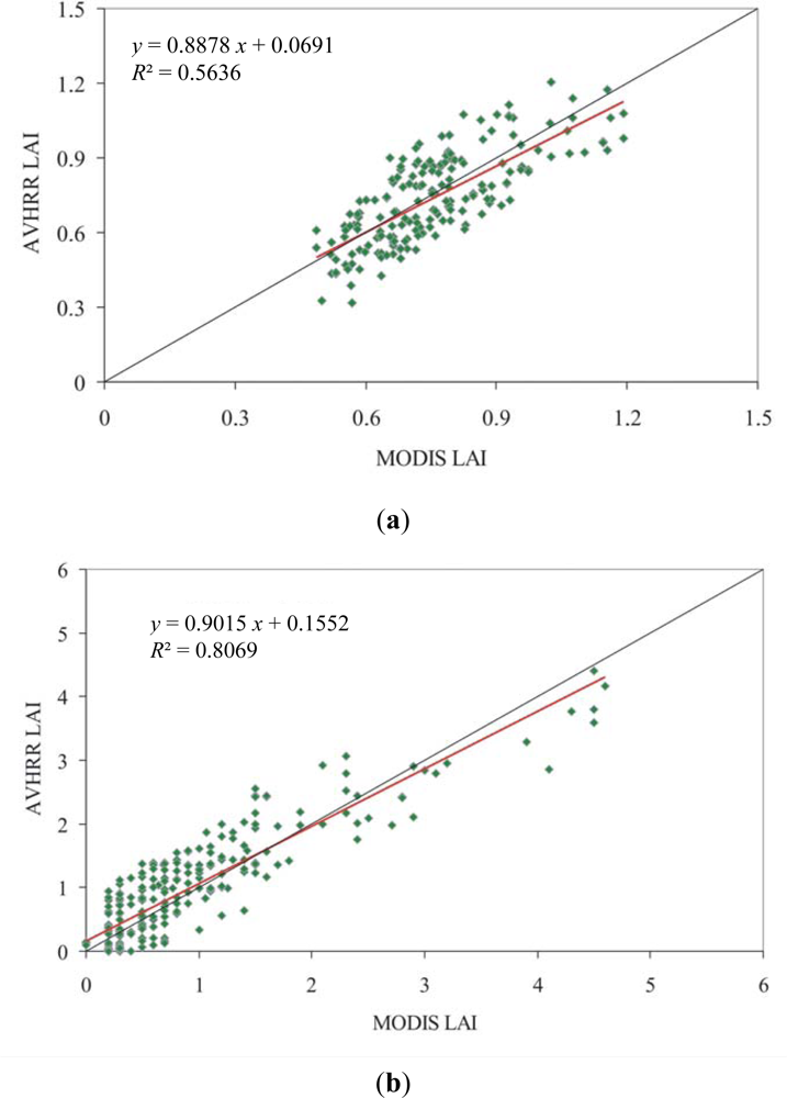
Scatter plots in Figure 9 show the per-pixel comparison of the LAI estimates for June 2008 and July 2009 at the grassland test site in Shetsky raion and at the wood/forest test area in Almaty region. In both scatter plots, we found a significant consistency between the compared LAI products: R2 = 0.56 and RMSE = 0.16 (0.23 LAI) for grassland and R2 = 0.80 and RMSE = 0.57 (0.42LAI) for woodland/forest). The values of RMSE were considerably below the value of 0.5LAI established as the common accuracy guide for LAI estimates from satellite-based models. However, the scatter plots also expose discrepancies between the compared LAI data sets. In both plots, the linear regression between the AVHRR and MODIS estimates is somewhat different from the 1:1 line demonstrating a value of the slope <1 and a positive value of the offset. This means that the AVHRR LAI dataset slightly overestimates lower LAI values in comparison to the MOD15A2 product and underestimates higher LAI values. Since the MODIS LAI is also known for its overestimation of grass and wood vegetation because of algorithm deficits [19,22,35,65], we assume that these slight under/overestimations of the MODIS LAI estimates by the AVHRR LAI data set produced in this study is not an shortcoming but an advantage.
5. Conclusions
The enhanced 8-km-resolution LAI data set covering the whole area of the Republic of Kazakhstan was developed using coarse-resolution AVHRR satellite data, auxiliary information and in situ measurements of canopy structure and canopy architecture. The algorithm was based on interpretation of satellite-measured Normalized Difference Vegetation Index (NDVI) using numerical inversion of an analytical canopy radiative transfer model (RTM) that accounts for major effects of surface reflectance, view-illumination conditions, optical properties of vegetation and parameters characterizing canopy architecture. The in situ canopy structure data were collected during several field survey campaigns in major vegetation biomes of Kazakhstan using contact destructive and non-contact optical methods and provided a consistent data set for calibration of the model and validation of the Kazakhstan-wide LAI product. The enhancement of the employed RTM algorithm is calculation of all input parameters individually for each pixel accounting for spatial and temporal patterns.
The coarse-resolution LAI product was validated using fine-resolution LAI images aggregated to 8-km spatial resolution. These fine-resolution LAI images were derived from empirical models between ground-based LAI and Landsat ETM+ data. The results of the validation demonstrate that LAI modeled from fine- and coarse-resolution satellite data is strongly correlated at the per-pixel level suggesting a good feasibility of the produced coarse-resolution LAI data set. In all validation tests, the error in LAI (in terms of RMSE) in individual coarse-resolution pixels is found to be about 0.15 LAI to 0.4 LAI indicating that the general accuracy requirement (<0.5 LAI) for remote sensing-based LAI estimates was fulfilled. Analysis of scatterplots and histograms of resulting LAI distributions in different test areas within the main biomes of Kazakhstan indicate that the overall distribution of LAI was consistent for the Landsat-derived and AVHRR-derived LAI images and remains close to being normally distributed.
The produced Kazakhstan-wide LAI data set was also evaluated with respect to the global 8-km AVHRR LAI product (LAI_PAL_BU_V3) for the area of Kazakhstan. On the one hand, the results showed a general good spatial and temporal consistency of the produced LAI data set with the LAI_PAL_BU_V3 product. On the other hand, the calculated LAI values are mostly lower than the LAI values of the LAI_PAL_BU_V3 data set. As a consequence, the LAI_PAL_BU_V3 product is characterized by a significantly higher mean value of LAI throughout the studied period. The differences in LAI values are more considerable for areas with either very infrequent or very dense vegetation cover. For all pixels within such areas, the LAI_PAL_BU_V3 algorithm assigns fixed values of LAI (0 or 6), while the AVHRR LAI produces a pixel-individual LAI value maintaining heterogeneity in the algorithm output. Due to fixed LAI values, the resulting LAI histogram calculated from the LAI_PAL_BU_V3 product reveals highly non-random distribution with extremely high LAI frequency in the left- and right-range classes. On contrast, the LAI histogram from the AVHRR LAI product demonstrates the near normal distribution. Another difference is that the LAI_PAL_BU_V3 product sustains high values of LAI during the months outside the growing season. The base level LAI values of the LAI_PAL_BU_V3 product were too high for the months characterized by no green vegetation.
Our simulated LAI values were very close to the LAI values from the MOD15A2 LAI product. A comparison of these products over the Almaty and Shetsky test sites revealed a strong spatial association at the per-pixel scale. This result is very positive and supports the above conclusions about good accuracy of the produced national-wide AVHRR LAI data set. Carrying out the comparison between the retrieved national-wide AVHRR LAI and the MODIS LAI product, we did not aim to do a qualitative assessment of the second product. An evaluation of the MODIS LAI product over the grassland test area in Shetsky region can be found in a previous study by the authors [35]. In the presented study, the aim of the comparison was to evaluate the appropriateness of the produced AVHRR LAI estimations against other independent data sets.
Generally, the results of validation and comparison with other independent satellite-derived LAI data sets consider the good ability of NOAA AVHRR-derived LAI data set for further use in the Kazakhstan-wide models for assessment of carbon sequestration throughout the period of three decades (1982–2008).
Acknowledgments
This research work has been carried out in cooperation with the Space Research Institute of the Science Academy of Kazakhstan. The authors gratefully acknowledge all colleagues from the Space Research Institute and particularly the leader of the Institute N. R. Muratova for their assistance in field survey and their helpful recommendations and approvals.
References
- Jonckheere, I.; Fleck, S.; Nachaerts, K.; Muysa, B.; Coppin, P.; Weiss, M.; Baret, F. Review of methods for in situ leaf area index determination. Part I. Theories, sensors and hemispherical photography. Agr. Forest Meteorol 2007, 121, 19–35. [Google Scholar]
- Breda, N.J.J. Ground-based measurements of leaf area index: a review of methods, instruments and current controversies. J. Exp. Bot 2003, 54, 2403–2417. [Google Scholar]
- Weiss, M.; Baret, F.; Smith, G. L.; Jonckheere, I.; Coppin, P. Review of methods for in situ leaf area index determination. Part II. Estimation of LAI, errors and sampling. Agr. Forest Meteorol 2004, 121, 37–53. [Google Scholar]
- Chen, J.; Cihlar, J. Retrieving LAI of boreal conifer forests using Landsat TM images. Remote Sens. Environ 1996, 55, 153–162. [Google Scholar]
- White, J.; Running, S.; Nemani, R.; Keane, R.; Ryan, K. Measurement and remote sensing of LAI in rocky mountain montane ecosystems. Can. J. Forest Res 1997, 27, 1714–1727. [Google Scholar]
- Turner, D.P.; Cohen, W.B.; Kennedy, R.E.; Fessnacht, K.S.; Briggs, J.M. Relationships between leaf area index and Landsat TM spectral vegetation indices across three temperate zone sites. Remote Sens. Environ 1999, 70, 52–68. [Google Scholar]
- Brown, L.J.; Chen, J.M.; Leblanc, S.G.; Cihlar, J. Shortwave infrared correction to the simple ratio: An image and model analysis. Remote Sens. Environ 2000, 77, 16–25. [Google Scholar]
- Eklundh, L.; Harrie, L.; Kuusk, A. Investigating relationships between Landsat ETM+ sensor data and LAI in a boreal conifer forest. Remote Sens. Environ 2001, 78, 239–251. [Google Scholar]
- Chen, M.; Pavlic, G.; Brown, L.; Cuhlar, J.; Leblanc, S.G.; White, H.P.; Hall, R.J.; Peddle, D.R.; King, D.J.; Trofimow, J.A.; et al. Derivation and validation of Canada-wide coarse-resolution leaf area index maps using high-resolution satellite imagery and ground measurements. Remote Sens. Environ 2002, 80, 165–184. [Google Scholar]
- Propastin, P. Spatial non-stationarity and scale-dependency of prediction accuracy in the remote estimation of LAI over a tropical rainforest in Sulawesi, Indonesia. Remote Sens. Environ 2009, 113, 2234–2242. [Google Scholar]
- Myneni, R.B.; Knyazikhin, Y.; Zhang, Y.; Tian, Y.; Wang, Y.; Lutach, A.; Privette, J.L.; Morisette, J.T.; Running, S.W.; Nemani, R.; et al. MODIS Leaf Area Index and Fraction of Photosynthetically Absorbed Radiation (MOD15) Algorithm Theoretical Basis Document. 1999. Available online: http://modis.gsfc.nasa.gov/data/atbd/atbd_mod15.pdf (accessed on 30 November 2011).
- Knyazikhin, Y.; Martonchik, J.V.; Diner, D.J.; Myneni, R.B.; Verstraete, M.; Pinty, B.; Gobron, N. Estimation of vegetation canopy leaf area index and fraction of absorbed photosynthetically active radiation from atmosphere-corrected MISR data. J. Geophys. Res 1998, 103, 32239–32256. [Google Scholar]
- Myneni, R.; Hoffman, R.; Knyazikhin, Y.; Privette, J.; Glassy, J.; Tian, H. Global products of vegetation leaf area and fraction absorbed PAR from one year of MODIS data. Remote Sens. Environ 2002, 83, 214–231. [Google Scholar]
- Baret, F.; Hagolle, O.; Geiger, B.; Bicheron, P.; Miras, B.; Huc, M.; Berthelot, B.; Nino, F.; Weiss, M.; Samain, O.; et al. LAI, fAPAR, and FCover CYCLOPES global products derived from Vegetation. Part 1: principles of the algorithm. Remote Sens. Environ 2007, 110, 305–316. [Google Scholar]
- Verger, A.; Camacho, F.; Garsia-Haro, J.; Melia, J. Evaluation of an operational leaf area index retrieval approach using VEGETATION and MODIS data. EARSeL eProc 2009, 8, 180–187. [Google Scholar]
- Myneni, R.B.; Nemani, R.R.; Running, S.W. Estimation of global leaf area index and absorped par using radiative transfer models. IEEE Trans. Geosci. Remote Sens 1997, 35, 1380–1393. [Google Scholar]
- Buermann, W.; Wang, Y.; Dong, J.; Zhou, L.; Zeng, X.; Dickinson, R.E.; Potter, C.S.; Myneni, R.B. Analysis of a multiyear global vegetation leaf area index data set. J. Geophys. Res 2002, 107, 4646. [Google Scholar]
- Ganguly, S.; Samanta, A.; Schull, M.A.; Shabanov, N.V.; Milesi, C.; Nemani, R.R.; Knyazikhin, Y.; Myneni, R.B. Generating vegetation leaf area index Earth system data record from multiple sensors. Part 2: Implementation, analysis and validation. Remote Sens. Environ 2008, 112, 4318–4332. [Google Scholar]
- Fensholt, R.; Sandholt, I.; Rasmussen, M.S. Validation of MODIS LAI, fAPAR and the relation between fAPAR and NDVI in a semi-arid environment using in situ measurements. Remote Sens. Environ 2004, 91, 490–507. [Google Scholar]
- Hill, M.J.; Senarath, U.; Lee, A.; Zeppel, M.; Nightingale, J.M.; Williams, R.J.; McVicar, T.R. Assessment of the MODIS LAI product for Australian ecosystems. Remote Sens. Environ 2006, 101, 495–518. [Google Scholar]
- Fang, H.; Liang, S.; Townshend, J.R.; Dickinson, R.E. Spatially and temporally continuous LAI data sets based on an integrated filtering method: examples from North America. Remote Sens. Environ 2008, 112, 75–93. [Google Scholar]
- Yang, W.; Tan, B.; Huang, D.; Rautiainen, M.; Shabanov, N.V.; Wang, Y.; Privette, J.L.; Huemmrich, K.F.; Fensholt, R.; Sandholt, I.; et al. MODIS leaf area index products: From validation to algorithm improvement. IEEE Trans. Geosci. Remote Sens 2006, 44, 1885–1898. [Google Scholar]
- Pisek, J.; Chen, J.M. Comparison and validation of MODIS and VEGETATION global LAI products over four BigFoot sites in North America. Remote Sens. Environ 2007, 109, 81–94. [Google Scholar]
- Sprintsin, M.; Karnielli, A.; Berliner, P.; Rotenberg, E.; Yakir, D.; Cohen, S. The effect of spatial resolution on the accuracy of leaf area index estimation for a forest planted in the desert transition zone. Remote Sens. Environ 2007, 109, 416–428. [Google Scholar]
- Blümel, B.; Reimer, E. Validation of boundary layer parameters of climate model REMO: estimation of leaf area index from NOAA-AVHRR data from the Baltimos region. Theor. Appl. Climatol 2009. [Google Scholar] [CrossRef]
- Propastin, P.; Erasmi, S. A physically based approach to model LAI from MODIS 250 m data in a tropical region. Int. J. Appl. Earth Obs. Geoinf 2010, 12, 47–59. [Google Scholar]
- Lal, R. Carbon sequestration in soils of Central Asia. Land Degrad. Dev 2004, 15, 563–572. [Google Scholar]
- Laca, E.A.; McEarchern, M.B.; Demment, M.W. Global grazing lands and greenhouse gas fluxes. Rangeland Ecol. Manag 2010, 63, 1–3. [Google Scholar]
- Henebry, G.M. Carbon in idle croplands. Nature 2009, 457, 1089–1090. [Google Scholar]
- Propastin, P.; Kappas, M. Modelling net ecosystem exchange for grassland in Central Kazakhstan by combining remote sensing and field data. Remote Sens 2009, 1, 159–183. [Google Scholar]
- Propastin, P.; Kappas, M.; Herrmann, S.; Tucker, C. Modified light use efficiency model for assessment of carbon sequestration in grasslands of Kazakhstan: Combining ground biomass data and remote sensing. Int. J. Remote Sens 2011, 33, 1465–1487. [Google Scholar]
- Causarano, H.J.; Doraiswamy, P.C.; Muratova, N.; Pachikin, K.; McCarty, G.W.; Akhmetov, B.; Williams, J.R. Improved modelling of soil organic carbon in a semi-arid region of Central East Kazakhstan using EPIC. Agron. Sustain. Dev 2010, 30. [Google Scholar] [CrossRef]
- Propastin, P.; Kappas, M. Mapping Leaf Area Index in a semi-arid environment of Kazakshtan using fine-resolution satellite data and in situ measurements. GISci. Remote Sens 2009, 46, 231–246. [Google Scholar]
- Propastin, P.; Kappas, M. Mapping leaf area index over semi-desert and steppe biomes in Kazakhstan using satellite imagery and ground measurements. EARSeL eProc 2009, 8, 75–92. [Google Scholar]
- Propastin, P.; Kappas, M. Comparison of MODIS products with in situ measurements of LAI and fPAR in temperate grassland of Kazakhstan. Int. J. Dig. Earth 2011. submitted. [Google Scholar]
- McCoy, R.M. Field Methods in Remote Sensing; The Guildford Press: New York, NY, USA, 2005. [Google Scholar]
- REGENT INSTRUMENTS. Available online: http://www.regentinstruments.com (accessed on 30 November 2011).
- INRA. CAN-EYE v6.2. Available online: https://www4.paca.inra.fr/can-eye (accessed on 30 November 2011).
- Lang, A.R.; Xiang, Y. Estimation of leaf area index from transmission of direct sunlight in discontinuous canopies. Agr. Forest Meteorol 1986, 35, 229–243. [Google Scholar]
- Tyurmenco, A.N. Biologitcheskiy krugovorot zolnych elementov pod celinnoy i culturnoy rastitelnostyu w zone sukhich i polupustynnych stepey. In Genesis, swoystwa i plodorodiye potchw; (In Russian). Kazan’; Izdatel’stvo Kazanskogo Universiteta, 1975; pp. 135–176. [Google Scholar]
- White, M.A.; Thornton, P.E.; Running, S.W.; Nemani, R.R. Parametrization and sensitivity analysis of the BIOME-BGC terrestrial ecosystem model: Net primary production controls. Earth Interact 2000, 4, 1–85. [Google Scholar]
- Pinzon, J.E.; Brown, M.E.; Tucker, C.J. Global Inventory Modelling and Mapping Studies (GIMMS) AVHRR 8-km Normalized Difference Vegetation Index (NDVI) Data Set. Product Guide. 2004. Available online: http://landcover.org/library/guide/GIMMSdocumentation_NDVIg_8km_rev4.pdf (accessed on 2 April 2011).
- Holben, B.N. Characteristics of maximum-value composite images from temporal AVHRR data. Int. J. Remote Sens 1986, 7, 1417–1434. [Google Scholar]
- Los, S.O.; Collatz, G.J.; Sellers, P.J.; Malmström, C.M.; Pollack, N.H.; DeFries, R.S.; Bounoua, L.; Parris, M.T.; Tucker, C.J.; Dazlich, D.A. A global 9-yr biophysical land surface dataset from NOAA AVHRR data. J. Hydrometeor 2000, 1, 183–199. [Google Scholar]
- Landsat archive. Available online: http://glovis.usgs.gov/ (accessed on 30 November 2011).
- Fallah-Adl, H.; Jaja, J.; Liang, S. Fast algorithms for estimating aerosol optical depth and correcting Thematic Mapper (TM) imagery. J. Supercomput 1997, 10, 300–315. [Google Scholar]
- Teillet, P.M.; Guindon, B.; Goodenough, D.G. On the slope-aspect correction of multispectral scanner data. Can. J. Remote Sens 1982, 8, 84–106. [Google Scholar]
- DeFries, R.S.; Hansen, M.; Townshend, R.J.G.; Sohlberg, R. Global land cover classification at 8-km spatial resolution: The use of training data derived from Landsat imagery in decision tree classifiers. Int. J. Remote Sens 1998, 19, 3141–3168. [Google Scholar]
- Global Land Cover Facility Archive Centre. Available online: http://www.landcover.org/data/landcover/data.shtml (accessed n 30 November 2011).
- Norman, J.M.; Campbell, S.G. Canopy structure. In Plant Physiological Ecology. Field Methods and Instrumentation; Pearcy, R., Ehleringer, J.R., Mooney, H.A., Rundel, P.W., Eds.; Chapman and Hall: London, UK, 1989; pp. 301–325. [Google Scholar]
- Gutman, G.; Ignatov, A. The derivation of the green vegetation fraction from NOAA/AVHRR data for use in numerical weather prediction models. Int. J. Remote Sens 1998, 19, 1533–1543. [Google Scholar]
- Wittich, K.P. Some simple relationships between land-surface emissivity, greenness and the plant cover fraction for use in satellite remote sensing. Int. J. Biometeorol 1997, 38, 58–64. [Google Scholar]
- Zeng, X.; Dickinson, R.E.; Walker, A.; Shaikh, M.; DeFries, R.S.; Qi, J. Derivation and evaluation of global 1-km fractional vegetation cover data for land modelling. J. Appl. Meteorol 2000, 39, 826–839. [Google Scholar]
- Zeng, X.; Rao, P.; DeFries, R.S.; Hansen, M.C. Interannual variability and decadal trend of global fractional vegetation cover from 1982 to 2000. J. Appl. Meteorol 2003, 42, 1525–1530. [Google Scholar]
- Choundry, B.J.; Ahmed, N.U.; Idso, S.B.; Riganto, R.J.; Doughtry, C.S.T. Relations between evaporation coefficients and vegetation indices studied by model simulations. Remote Sens. Environ 1994, 50, 1–17. [Google Scholar]
- Jarvis, P.G.; Laverenz, J.W. Productivity of temperate, deciduous and evergreen forests. In Physiological Plant Ecology IV; Lange, O.L., Omond, C.B., Zeigler, H., Eds.; Srpinger-Verlag: New York, NY, USA, 1983; pp. 133–144. [Google Scholar]
- Jones, H.G. Plant and microclimate, 2nd Ed. edCambrige University Press: Cambrige, UK, 1992. [Google Scholar]
- Wang, Y.P.; Jarvis, G.P. Mean leaf angles for ellipsoidal inclination distribution. Agr. Forest Meteorol 1988, 43, 319–321. [Google Scholar]
- Kucharik, C.J.; Norman, J.M.; Gower, S.T. Characterization of radiation regimes in non-random forest canopies: Theory, measurements, and simplified modelling approach. Tree Physiol 1998, 19, 695–706. [Google Scholar]
- US Geological Survey, EROS Data Center. Global 30 Arc Second Elevation Data Set (GTOPO30). 1998. Available online: http://www1.gsi.go.jp/geowww/globalmap-gsi/gtopo30/gtopo30.html (accessed on 30 November 2011).
- Morisette, J.T.; Baret, F.; Privette, J.L.; Myneni, R.B.; Nickeson, J.E.; Garrigues, S.; Shabanov, N.V.; Weiss, M.; Fernandes, R.A.; Leblanc, S.G.; et al. Validation of global moderate resolution LAI Products: A framework proposed within the CEOS Land Product Validation subgroup. IEEE Trans. Geosci. Remote Sens 2006, 44, 1804–1817. [Google Scholar]
- Atkinson, P.; Tate, N. Spatial scale problems and geostatistical solutions: A review. Prof. Geogr 2000, 52, 607–623. [Google Scholar]
- Earth Observing System Data Gateway. Available online: http://edcimswww.cr.usgs.gov/pub/imswelcome/ (accessed on 30 November 2011).
- Huete, A.R. A soil-adjusted vegetation index (SAVI). Remote Sens. Environ 1988, 25, 295–309. [Google Scholar]
- Shabanov, N.V.; Kotchenova, S.; Huang, D.; Yang, W.; Tan, B.; Knyazikhin, Y.; et al. Analysis and optimization of the MODIS leaf area index algorithm retrievals over broadleaf forests. IEEE Trans. Geosci. Remote Sens 2005, 43, 1855–1865. [Google Scholar]
Figure 1.
Classification of current vegetation for the Republic of Kazakhstan based on the 8-km Advanced Very High Resolution Radiometer (AVHRR) LANDCOVER 1981–1994 global map [45]. Test sites for in situ measurements are presented by squares and names.
Figure 1.
Classification of current vegetation for the Republic of Kazakhstan based on the 8-km Advanced Very High Resolution Radiometer (AVHRR) LANDCOVER 1981–1994 global map [45]. Test sites for in situ measurements are presented by squares and names.

Figure 2.
Distribution of the AVHRR LAI for June 2008 over the Republic of Kazakhstan.

Figure 3.
Monthly courses of the area-averaged LAI derived from the national-wide AVHRR LAI data set for the period 1982–2008.
Figure 3.
Monthly courses of the area-averaged LAI derived from the national-wide AVHRR LAI data set for the period 1982–2008.


Figure 4.
Validation of fine-resolution radiative transfer model (RTM)-based LAI products at the grassland test site in Shetsky region. (a) LAI retrievals from the fine-resolution RTM algorithm versus ground measured LAI for 2008. (b) LAI retrievals from the fine-resolution RTM algorithm versus ground measured LAI for 2004. (c) LAI retrievals from the fine-resolution RTM algorithm versus retrievals by the regression-based algorithm for 2008 in a pixel-by-pixel comparison (n = 64,000).


Figure 5.
Validation of AVHRR LAI product in the grassland biome in the Shetsky test region. (a) Pixel-by-pixel (n = 1,215) comparison of the aggregated fine-resolution LAI map retrieved using RTM algorithm and the AVHRR LAI for 2008. (b) Same as in panel (a), but retrievals from the regression-based Landsat ETM+ LAI for 2008. (c) Frequency distribution of LAI modeled from Landsat ETM+ data using the RTM and regression algorithm, and AVHRR data.

Figure 6.
Validation of AVHRR LAI product at the Almaty forest test site. (a) Relationship between field-measured LAI and the Landsat ETM+-derived SAVI. (b) Pixel-by-pixel comparison of the aggregated fine-resolution LAI map and the AVHRR LAI product. (c) Frequency distribution of the Landsat ETM+ regression-based LAI and AVHRR LAI.


Figure 7.
Comparison of the AVHRR LAI to LAI_PAL_BU_V3. (a) Pixel-by-pixel comparison of the AVHRR LAI map and the LAI_PAL_BU_V3 product over the whole area of Kazakhstan for July 2008. (b) Frequency distribution of the AVHRR LAI and LAI_PAL_BU_V3.
Figure 7.
Comparison of the AVHRR LAI to LAI_PAL_BU_V3. (a) Pixel-by-pixel comparison of the AVHRR LAI map and the LAI_PAL_BU_V3 product over the whole area of Kazakhstan for July 2008. (b) Frequency distribution of the AVHRR LAI and LAI_PAL_BU_V3.

Figure 8.
Temporal profiles of LAI estimates from the LAI_PAL_BU_V3 product, the Kazakhstan-wide AVHRR LAI product and ground-based measurements at test sites.
Figure 8.
Temporal profiles of LAI estimates from the LAI_PAL_BU_V3 product, the Kazakhstan-wide AVHRR LAI product and ground-based measurements at test sites.


Figure 9.
Comparison of the AVHRR LAI and MODIS LAI product. (a) LAI estimates over the grassland test area in Shetsky raion for June 2008. (b) LAI estimates over the wood/forest test area in Almaty region for July 2008.
Figure 9.
Comparison of the AVHRR LAI and MODIS LAI product. (a) LAI estimates over the grassland test area in Shetsky raion for June 2008. (b) LAI estimates over the wood/forest test area in Almaty region for July 2008.


Table 1.
In situ measurements of leaf area index (LAI) in Kazakhstan used in this study. For location of the test sites (see Figure 1).
| Test Site and Number of Sampling Plots | Date | Vegetation Type | Measurement Method | LAI Range |
|---|---|---|---|---|
| Shetsky 1, 14 plots | June 2004 | Grassland | Direct contact destructive | 0.25–1.12 |
| Cropland | 0.31–0.85 | |||
| Shetsky 2, 20 plots | June 2008 | Grassland | Indirect non-contact optical | 0.30–1.55 |
| Cropland | 0.21–0.75 | |||
| Shrubland | 0.84–2.06 | |||
| Almaty, 16 plots | June 2008 | Mixed forest | Indirect non-contact optical | 3.30–5.90 |
| Deciduous broadleaf forest | 3.10–5.10 | |||
| Deciduous needleaf forest | 4.35–7.24 | |||
| Woodland | 2.42–4.10 |
| Location Name/Test Site | Scene Date | Landsat Path/Row |
|---|---|---|
| Shetsky 1 | June 16 2004 | 153/26 |
| 153/27 | ||
| Shetsky 2 | June 19 2008 | 153/26 |
| Almaty | July 30 2008 | 149/30 |
Share and Cite
MDPI and ACS Style
Propastin, P.; Kappas, M. Retrieval of Coarse-Resolution Leaf Area Index over the Republic of Kazakhstan Using NOAA AVHRR Satellite Data and Ground Measurements. Remote Sens. 2012, 4, 220-246. https://doi.org/10.3390/rs4010220
AMA Style
Propastin P, Kappas M. Retrieval of Coarse-Resolution Leaf Area Index over the Republic of Kazakhstan Using NOAA AVHRR Satellite Data and Ground Measurements. Remote Sensing. 2012; 4(1):220-246. https://doi.org/10.3390/rs4010220
Chicago/Turabian StylePropastin, Pavel, and Martin Kappas. 2012. "Retrieval of Coarse-Resolution Leaf Area Index over the Republic of Kazakhstan Using NOAA AVHRR Satellite Data and Ground Measurements" Remote Sensing 4, no. 1: 220-246. https://doi.org/10.3390/rs4010220