Article

Exploring Simple Algorithms for Estimating Gross Primary Production in Forested Areas from Satellite Data

1
Division of Science & Environmental Policy, California State University, Monterey Bay, Seaside, CA 93955, USA
2
NASA Ames Research Center, Moffett Field, CA 94040, USA
3
Department of Watershed Sciences, Utah State University, Logan, UT 84322, USA
4
Bay Area Environmental Research Institute, Sonoma, CA 95476, USA
5
National Institute of Advanced Industrial Science and Technology, Tsukuba, Ibaraki 305-8569, Japan
6
Graduate School of Agriculture, Hokkaido University, Sapporo, Hokkaido 060-8589, Japan
7
Department of Geography and Environment, Boston University, Boston, MA 02215, USA
*
Author to whom correspondence should be addressed.
Remote Sens. 2012, 4(1), 303-326; https://doi.org/10.3390/rs4010303
Submission received: 15 December 2011 / Revised: 12 January 2012 / Accepted: 12 January 2012 / Published: 23 January 2012

Abstract

:
Algorithms that use remotely-sensed vegetation indices to estimate gross primary production (GPP), a key component of the global carbon cycle, have gained a lot of popularity in the past decade. Yet despite the amount of research on the topic, the most appropriate approach is still under debate. As an attempt to address this question, we compared the performance of different vegetation indices from the Moderate Resolution Imaging Spectroradiometer (MODIS) in capturing the seasonal and the annual variability of GPP estimates from an optimal network of 21 FLUXNET forest towers sites. The tested indices include the Normalized Difference Vegetation Index (NDVI), Enhanced Vegetation Index (EVI), Leaf Area Index (LAI), and Fraction of Photosynthetically Active Radiation absorbed by plant canopies (FPAR). Our results indicated that single vegetation indices captured 50–80% of the variability of tower-estimated GPP, but no one index performed universally well in all situations. In particular, EVI outperformed the other MODIS products in tracking seasonal variations in tower-estimated GPP, but annual mean MODIS LAI was the best estimator of the spatial distribution of annual flux-tower GPP (GPP = 615 × LAI − 376, where GPP is in g C/m2/year). This simple algorithm rehabilitated earlier approaches linking ground measurements of LAI to flux-tower estimates of GPP and produced annual GPP estimates comparable to the MODIS 17 GPP product. As such, remote sensing-based estimates of GPP continue to offer a useful alternative to estimates from biophysical models, and the choice of the most appropriate approach depends on whether the estimates are required at annual or sub-annual temporal resolution.
Keywords:
GPP; LAI; EVI; NDVI; MODIS

1. Introduction

Understanding the mechanisms of global climate change and improving our predictions of possible future climates requires accurate quantifications of carbon uptake by terrestrial vegetation. Gross Primary Production (GPP), the amount of carbon assimilated by vegetation through photosynthesis over time, fundamentally influences the carbon cycle and human habitability of our planet [1]. While the mechanisms regulating GPP are well understood and modeled at the leaf and canopy level, regional and global GPP models still need to address large uncertainties in the estimates [2].
Historically, scientists have tried to explain the spatial and temporal patterns of GPP by exploiting its relation with vegetation biophysical metrics such as Leaf Area Index (LAI) [3], foliar standing crop [4], the Fraction of Photosynthetically Active Radiation absorbed by plant canopies (FPAR) [5], or with vegetation indices like the integrated Normalized Differential Vegetation Index (NDVI) [6]. Following the recognition that drought conditions suppress summer photosynthesis [7], process-oriented models were developed to estimate GPP with a combination of meteorological data and satellite-observed biophysical parameters, such as FPAR [8] and LAI [9]. These process-oriented models, while allowing simulations of ecosystems under future climate scenarios, present large uncertainty when used for current estimations of GPP because the required input parameters are not available with adequate accuracy at the global scale. The possibility of estimating GPP based on meteorological data only (e.g., Kato et al. [10]), combinations of satellite-observed biophysical parameters (e.g., Wu et al. [11]; Xiao et al. [12]), or combinations of meteorological data and simple biophysical processes (e.g., temperature × (precipitation − evapotranspiration) [13]), has also been explored.
For global-scale studies of GPP, satellite data have the advantage of providing continuous, repetitive, and consistent observations of vegetation dynamics. The Advanced Very High Resolution Radiometer (AVHRR, available since 1981 and originally designed for weather monitoring) has been widely used for long-term analysis of global vegetation dynamics [14,15] but suffers from orbital drift, water vapor contamination and lack of onboard calibration [16]. In 1999 NASA launched the Moderate Resolution Imaging Spectroradiometer (MODIS) onboard the TERRA platform with the specific objective of monitoring Earth’s surface and atmosphere environment. MODIS data have now been used to generate a decade’s worth of standard land data products including vegetation indices, biophysical properties of vegetation, and carbon fluxes [17].
Concurrent with MODIS, participants in the global FLUXNET network of micrometeorological towers with eddy covariance instrumentation have recorded land-atmosphere exchanges of carbon dioxide, water vapor, and energy at hundreds of diverse sites [18,19]. Although uncertainties exist in the FLUXNET observations, the network has provided unprecedented estimates of GPP at high temporal resolution for almost a decade.
The development of these two data streams—MODIS and FLUXNET—has led to extensive tests of the ability of remote sensing to approximate GPP, especially at local scales. Among the MODIS products, the Enhanced Vegetation Index (EVI)—an optimized vegetation index developed from NDVI [20]—has shown a strong seasonal correlation with GPP [2124]. Sims et al. [23] found a high correlation between GPP and EVI in deciduous forests but not in evergreen forests. Huete et al. [24] extended the relationship between GPP and EVI to the monsoon forests of Southeast Asia. Xiao et al. [21] indicated that EVI could track FPAR by measuring photosynthetically active vegetation while excluding the senescent parts of vegetation. Some biophysical models have already tried to use EVI in place of NDVI to estimate vegetation carbon production [21,2527].
Although past research seems to have established the seasonal correlation of GPP with EVI at individual flux tower sites, questions still remain whether or not the relationship is consistent across sites, whether it is superior to the other existing satellite metrics of vegetation abundance and structure (NDVI, LAI, and FPAR), and whether it lends itself to estimating annual GPP. Although there are now a number of process-based models for GPP estimation, the use of a single satellite-derived metric still has great appeal for ease of application, assessing the effects of uncertainties caused by poor quality input data, and simplifying the exploration of the underlying mechanisms of vegetation responses to climate change and variability. In this study we analyzed and compared how well four MODIS vegetation products relate to short-term and annual GPP estimated at a network of ideal-quality FLUXNET sites.

2. Data and Methods

Our overall approach was to compare a suite of remotely-sensed vegetation metrics to GPP estimated at a quality-screened subset of the FLUXNET sites. In the following sections, we describe: (1) the selection and processing of MODIS data stored as subsets for the FLUXNET sites, (2) the conceptual basis of the MODIS products, (3) the processing and selection of FLUXNET data, and (4) our analytical approach.

2.1. MODIS Land Products Subsets

Collection 5 MODIS Land Products Subsets for FLUXNET sites are readily available from the Distributed Active Archive Center (DAAC) at Oak Ridge National Laboratory [28]. These subsets represent MODIS product cutouts of 7 km by 7 km around each FLUXNET tower, greatly simplifying the task of MODIS data retrieval for the FLUXNET sites.
We retrieved Collection 5 MOD13Q1 (NDVI and EVI) and MOD15A2 (LAI and FPAR), and Collection 5.1 MOD17A2 (GPP) (hereafter referred to as MOD13, MOD15, and MOD17, respectively) for the period 2001 to 2008 (Table 1). We used MOD17—a process-oriented model driven by FPAR and meteorological data—as a comparison with our simpler, single-metric approaches of estimating GPP. Unfortunately, MOD13 is only archived at 250 m, while the other products have a spatial resolution of 1 km. To make the subsets comparable, we averaged the sixteen MOD13 pixels over the 1 km area surrounding each tower. For each site, we then selected the central pixel from the 7 km by 7 km subset to represent the FLUXNET tower footprint and assembled the 2001–2008 MODIS products time series. The choice of working with the central 1km pixel is justified by the fact that the geolocation accuracy of MODIS is about 50 m (1 σ) at nadir [29] and because for most FLUXNET sites the representative vegetation cover extends for less than 1 km.
We only used data from years in which MODIS data were at least 80% complete (i.e., years for which more than 37 and 19 valid data per year were available for 8-day and 16-day composite periods, respectively). To compare across MODIS products, we did not use the quality flags (except for the snow flag), because the categories and the procedures defining the MODIS quality assurance fields vary for each MODIS product. Instead of using the quality flags, we applied the maximum value composite (MVC) method [32], and set all the non-processed data values to the corresponding maximum. If all the data in the MVC window were not processed, we labeled the pixel value as missing data. To assess the stability of the results with respect to the composite period, we processed the MODIS products to 8-day, 16-day, and 32-day composites.

2.1.1. MOD13 NDVI and EVI

MOD13 is the 250 m, 16-day composite NDVI and EVI product, derived from MOD09 reflectances. Even though vegetation indices are a unitless metric of vegetation greenness, they are widely used as monitoring tools because of the simplicity of their formulas. NDVI is defined as:
NDVI = ρ NIR ρ red ρ NIR + ρ red
where ρNIR is near infrared reflectance (841–876 nm) and ρred is red reflectance (620–670 nm) .
Among all vegetation indices, NDVI is the most widely used for monitoring and modeling vegetation dynamics [33,34]. However, NDVI-based monitoring of vegetation dynamics suffers from several drawbacks: it saturates over dense vegetation, is frequently contaminated by clouds and aerosols, and is sensitive to soil background reflectance. EVI [20] was introduced as a partial solution to these limitations of NDVI, and is calculated as:
EVI = G ρ NIR ρ red ρ NIR + C 1 ρ red C 2 ρ blue + L
EVI empirically corrects for aerosols with the reflectance in the blue band (ρblue, 459 to 479 nm) and adds L (1) as a background brightness correction factor. G (2.5) is the gain factor and C1 (6) and C2 (7.5) are band-specific atmospheric resistance correction coefficients.
We used the MOD13 quality assurance fields to identify the presence of snow, in which case we set the values of both NDVI and EVI to zero.

2.1.2. MOD15 LAI and FPAR

MOD15 is the 1 km, 8-day composite LAI and FPAR product [35]. The main algorithm for retrieving LAI and FPAR is based on a lookup table (LUT) inversion approach. The biome-specific LUTs, generated using a three-dimensional radiative transfer model [30,35], consists of spectral surface reflectances as a function of LAI, soil reflectances and view geometry. The inversion results in minimizing the difference between the observed surface reflectances and the simulated LUT entries to generate an average LAI value from a solution set [30]. If the main algorithm fails, a back-up algorithm based on the relationship between NDVI and LAI/FPAR is used in its place (in this study, the main algorithm had been applied to 72.8% of the LAI/FPAR data). Summarizing LAI validation studies, Yang et al. [35] showed that the MOD15 LAI product had an R2 of 0.87 when compared to measured LAI from 29 field campaigns, with an average overestimation of 12% (RMSE = 0.66). In a separate validation effort over the tropics, Aragão et al. [36] reported an overestimation by a factor of 1.18 at Tapajos, Brazil. The new Collection 5 (C5) MOD15 data, used in this study, was an improvement over the earlier collections, especially for the forest biomes [35,37,38]. A recent study by De Kauwe et al. [37] shows that the C5 MOD15 data has higher spatial consistency (R2 = 0.42) than Collection 4 (R2 = 0.28), when compared to upscaled in situ measurements of mixed coniferous forests. We screened the C5 MOD15 product by assigning the LAI and FPAR of each 8-day composite to zero when the quality assurance fields indicated that snow was present over a pixel. We calculated annual mean LAI and FPAR as for NDVI and EVI.

2.1.3. MOD17 GPP

MOD17 is the 1 km 8-day average GPP and is based on a light use efficiency (LUE) model [31]:
GPP = ε max * PAR * FPAR * f ( VPD ) * f ( Tmin )
where εmax is the biome-specific maximum light use efficiency (g C/MJ), PAR is photosynthetically active radiation (MJ), and potential GPP is linearly scaled between 1 (no limitation) to 0 (no GPP) using biome-specific functions for Vapor Pressure Deficit (f(VPD)) and minimum temperature (f(Tmin)) [39]. FPAR is from MOD15 and includes filling of cloud-contaminated pixels, while meteorological inputs are from the Goddard Earth Observing System Model (GEOS) of the NASA Data Assimilation Office (DAO) [40]. In this study, MOD17 was used as a reference dataset since it had been well validated with flux tower data [31,39].

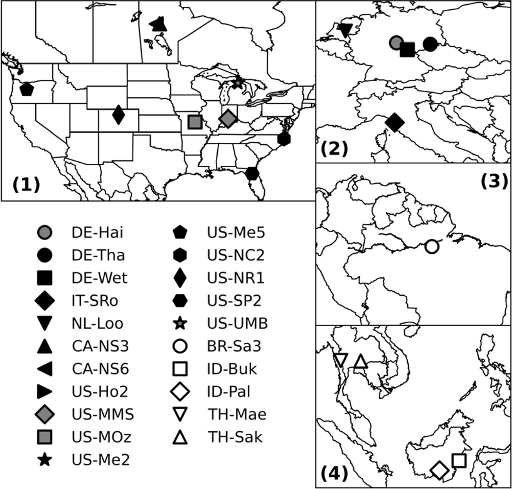
2.2. FLUXNET Dataset

We used standardized Level 4 FLUXNET data provided by AmeriFlux and CarboEurope networks. The Level 4 FLUXNET data include meteorological and eddy covariance flux data and estimated GPP (note that we use “GPP” interchangeably with “Gross Ecosystem Production”, though a small difference in photorespiration exists between the two). Level 4 data contain GPP derived from estimated Net Ecosystem Exchange (NEE) by different methods (two different storage term calculations and two different gap-filling methods). The storage term required for the estimation of NEE was either provided by each tower principal investigator (original) or estimated by a standard method assuming that CO2 concentration measured at eddy flux measurement height is constant within the canopy (standard). The gaps were filled either by the Marginal Distribution Sampling method [41] or by the Artificial Neural Network method [42]. We used the original Marginal Distribution Sampling GPP because the original storage term is more reliable than the standard method at tall tower sites [43] and the Artificial Neural Network approach may fill gaps that are too long. The u* filtering was applied to NEE following Reichstein et al. [41] and the time-series were finally gap-filled at the daily, weekly, and monthly time scale.
The partitioning of the measured NEE fluxes into GPP and Total Ecosystem Respiration (TER) was based on a temperature-dependent exponential model of TER estimated based on nighttime NEE data. GPP was finally obtained as the sum of NEE and TER according to Reichstein et al. [41]. Results of this partitioning method have been recently validated at a large number of FLUXNET sites against alternative estimates based on light response curves [44].
Scaling from point measurements at the flux tower to the 1 km MODIS resolution is not trivial because the heterogeneity of the flux tower footprint can lead to a time-variant measurement bias. Ideally, we should use flux towers whose eddy covariance footprints are homogeneous over the MODIS pixel, but this condition is not often met. In some studies (e.g., Turner et al. [45]), finer resolution satellite data have been used to bridge between flux tower data and coarse resolution data to account for the heterogeneity of the tower sites. Here, to avoid scaling issues, we selected flux tower sites where the land cover extended homogenously roughly over a 500 m radius circle around the tower (assessed by visual interpretation of Google Earth imagery). Thus, we only selected AmeriFlux and CarboEurope forest flux tower sites (Table 2 and Figure 1) that satisfied the following requirements:
  • The tower was surrounded by homogeneous land cover for a radius of at least 500 m;
  • Temporally overlapping coverage with the MODIS subset data existed;
  • The gap-filled ratio was less than 20% for all 12 months in a year.
The only tropical forest AmeriFlux tower meeting the above requirements was in Tapajos, Brazil. To increase the sample size for tropical forests and improve the robustness of our analysis, we added four AsiaFlux tropical sites from Southeast Asia: Bukit Soehart, Palangkaraya, Mae Klong, and Sakaerat. Only annual GPP data were published for these sites in Hirata et al. [46], and were derived from nighttime respiration estimated via exponential respiration model as in Reichstein et al. [41]. Following our full screening, we assembled a total of 21 FLUXNET sites with corresponding MODIS subset data for the years 2001 to 2008. For brevity, we refer to the sites with the codes defined in Table 2.
To assess the degree to which the selected FLUXNET sites were representative of the climatic range of the global forested regions, we first generated a 1982 to 2005 average global climatology of temperature and precipitation. We used the Climate Research Unit (CRU) TS3.1 dataset [63] and the MCD12C1 V005 [64] IGBP classification in 2001 (aggregated to a 0.5 degree resolution map by specifying the most frequent land cover in each pixel). We calculated the FLUXNET sites’ annual mean temperature and precipitation during the flux measurement period and compared the two datasets in the temperature-precipitation domain following Wang et al. [65]. The selected sites ranged from −5 °C to 25 °C in mean annual temperature and from 200 mm/year to 2,300 mm/year in mean annual total precipitation, largely covering the climatic variability of global forested areas (Figure 2).

2.3. Reduced Major Axis Regression Analyses

We examined the relationship between flux tower GPP and MODIS products with reduced major axis regression analysis, which minimizes the sum of the product of deviations from the model along both the x and y axes [66], both at the short-term and at the annual time scale. The correlation was evaluated with the coefficient of determination R2. The p-value testing the null hypothesis that the slope of the regression line is equal to zero was calculated using two-tailed t-tests.

2.4. Short-Term Analysis

The first question we asked is which MODIS product(s) best explains the short-term (i.e., intra-annual) variations in flux tower GPP. We averaged daily flux tower GPP estimates over each composite periods (8-day, 16-day, and 32-day), and applied MVC to each MODIS product to the corresponding composite periods. We then calculated the R2 between the flux tower average GPP and corresponding satellite-derived composite for each available year from 2001 to 2008, and then averaged the R2 of all years. R2 between flux tower GPP and satellite composites were also calculated after stratifying by forest type class (i.e., deciduous, evergreen, non-tropical, and tropical). In the same way as done with average R2, we also calculated average root mean square error (RMSE) using the reduced major axis regression.

2.5. Annual Analysis

The second question we asked is which MODIS product(s) best explains the annual variations in flux tower GPP. We calculated the annual mean of each MODIS product as the sum of the available values divided by the total number of available values. We then analyzed the regressions between flux tower annual total GPP and the annual mean of each MODIS product for the data organized into the following groups: all sites, non-tropical sites only, and tropical sites only. Similarly to the short-term analysis, we varied the composite period from 8, 16 to 32-days. We did not composite MOD17 because this would have caused to neglect its biophysically-induced reductions (e.g., reductions induced by drought periods rather than by cloud or aerosol contamination) and therefore lead to an overestimation of annual GPP.
Although annually integrated vegetation indices are sometimes used for this kind of analyses (e.g., Goward et al. [6]), we preferred to use annual mean vegetation indices. Satellite data are plagued by frequent missing data due to cloud contamination, high aerosol, etc., causing the annually integrated indices to be affected by the number of valid data. Also, the use of mean values facilitates the comparisons across deciduous and evergreen forest types.

3. Results

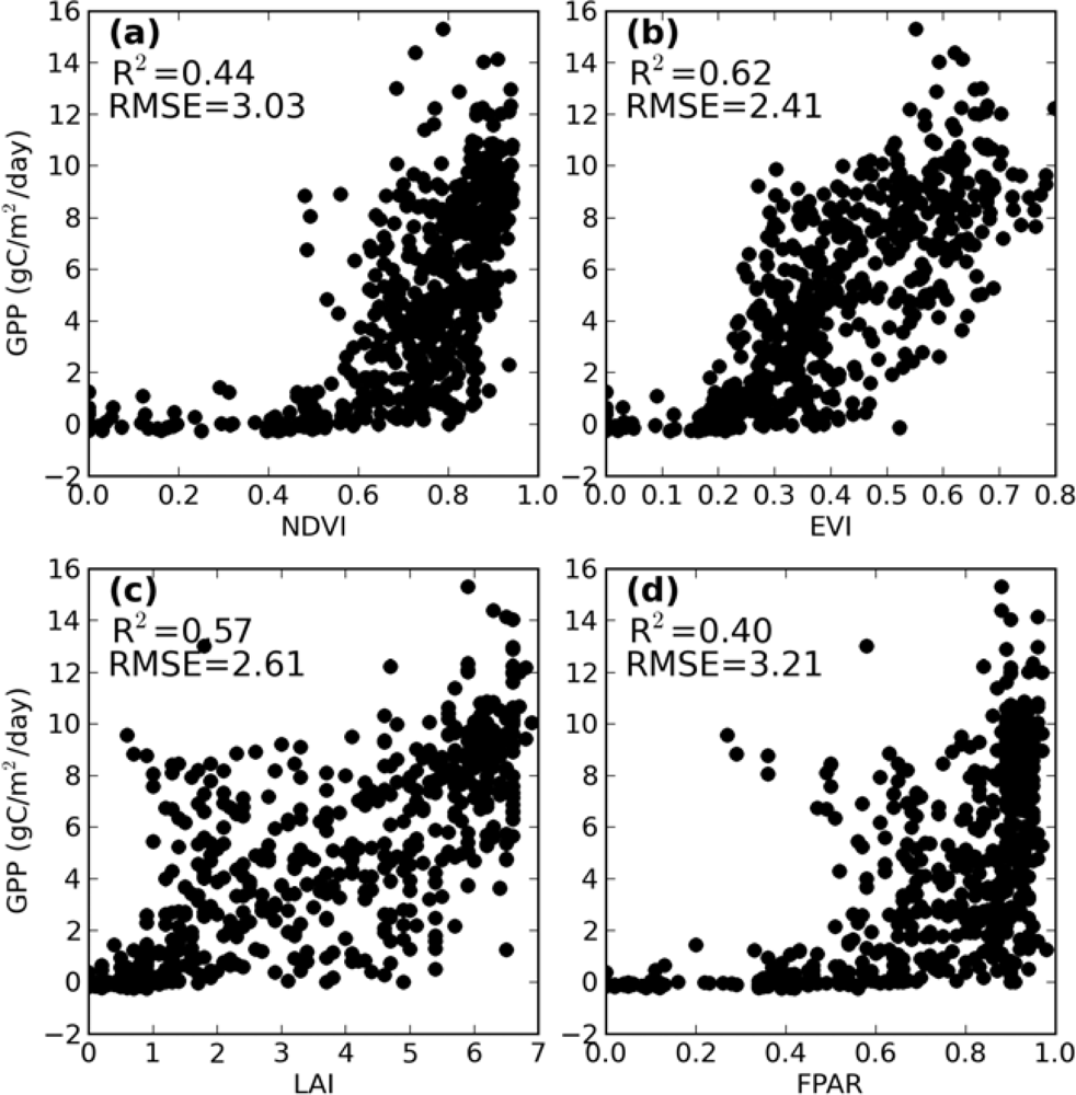
3.1. Short-Term Correlation between MODIS Products and Flux Tower GPP

Short-term GPP was more highly correlated with EVI than with NDVI, LAI, or FPAR (Table 3), in agreement with other studies that have shown high correlation between EVI and GPP [2124]. The correlations with NDVI and EVI were minimally affected by changing the compositing period from 16-days to 32-days, demonstrating that the auto-correction feature of vegetation indices to non-vegetation signals through normalization of the reflectances is effective. On the other hand, LAI and FPAR showed improved fitting when they were composited to 32-days. Because of their inability of capturing short-term changes in GPP (i.e., temporary reductions in GPP due to adverse weather conditions), both MOD13 and MOD15 products showed weaker correlation for evergreen forests than for deciduous forests. For all the products, no correlation was found with GPP of tropical forests (Table 3). This can be attributed to the small seasonal changes observed in tropical forest leaves, which are smaller than the interannual variation in leaf phenology (e.g., Huete et al. [24]). EVI generally showed smaller RMSE than NDVI, LAI, and FPAR.
For all analyzed sites, the reference data of MOD17 GPP was most highly correlated with short-term flux tower GPP, both for deciduous and evergreen forests (Table 3). This result can be explained by the fact that MOD17 GPP parameters have been well calibrated and tested at many FLUXNET sites [31,39,67]. This result also supports the need for meteorological input data in addition to the satellite metrics for better capturing the seasonal variations in photosynthesis (Running et al. [9]).
We plotted 32-day composites of MODIS products against flux tower GPP estimates for all the sites (Figure 3). NDVI and FPAR clearly showed saturation at values of 0.75 and above. EVI showed the highest correlation with flux tower GPP, but the modest R2 of 0.62 implied low accuracy in the estimation of short-term GPP through one equation using satellite metrics only. Theoretically, the four metrics should be correlated with each other. Indeed, Figure 3(a,b) shows a similar scatter even though NDVI and FPAR were calculated through very different approaches. This similarity can be explained by the well-known linear relationship between NDVI and FPAR [68]. FPAR and LAI are correlated through an exponential relationship usually described by Beer’s law, which explains the differences between the scatters of Figure 3(c) and Figure 3(d). However, even correlating the logarithmic transformation of GPP with MODIS NDVI and FPAR did not significantly increase the R2.

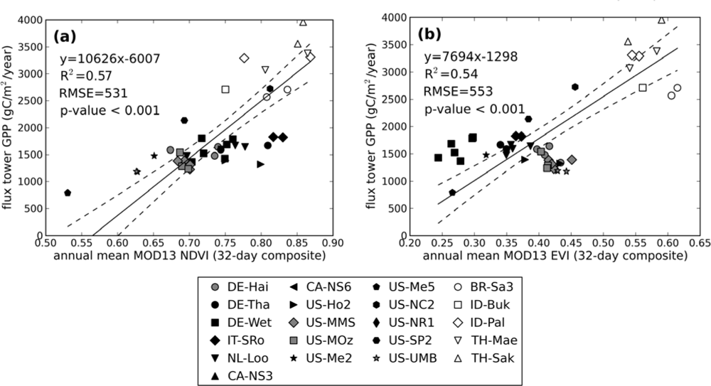
3.2. Annual Analysis between MODIS Products and Flux Tower GPP

3.2.1. NDVI and EVI vs. Annual Mean GPP

When all sites were analyzed at a 32-day resolution, annual mean NDVI and EVI showed comparable correlations with annual GPP (Figure 4). When the GPP of tropical and non-tropical sites were compared separately to EVI, however, the correlation was much lower and non-significant (Table 4 and Figure 4(b)). In contrast, NDVI showed moderate correlation both for all sites and non-tropical sites, but the linear relationship between NDVI and annual GPP collapsed at NDVI greater than 0.75. Similarly to the short-term analysis, compositing to 32-day did not significantly change the results (Table 4).

3.2.2. LAI and FPAR vs. Annual Mean GPP

LAI had the highest correlation with annual GPP, regardless of the compositing period length (Table 4 and Figure 5(a)). LAI showed high correlation with tower GPP both for non-tropical sites (R2 0.43 to 0.68) and tropical sites (R2 0.66 to 0.70). Increased compositing length tended to increase R2 for non-tropical sites and decrease R2 in tropical sites. The R2 values for the comparisons between FPAR and annual GPP were similar, but slightly lower than those for LAI (Table 4). At FPAR greater than 0.7, flux tower GPP was generally underpredicted by the regression at non-tropical sites (Figure 5(b)). As for LAI, when compositing to longer periods, FPAR correlations increased at non-tropical sites and tended to decrease at tropical sites (Table 4).
While several metrics showed promise in estimating annual flux tower GPP, annual mean LAI derived from 32-day composites had the highest correlation, explaining 88% of measured variance. The simple model is:
GPP = 615 * annual     mean     LAI 376
where annual GPP is in g C/m2/year. It is noteworthy that we tried the same analysis with max LAI, but max LAI was poorly correlated with annual GPP, as previously shown by other studies [10,13].

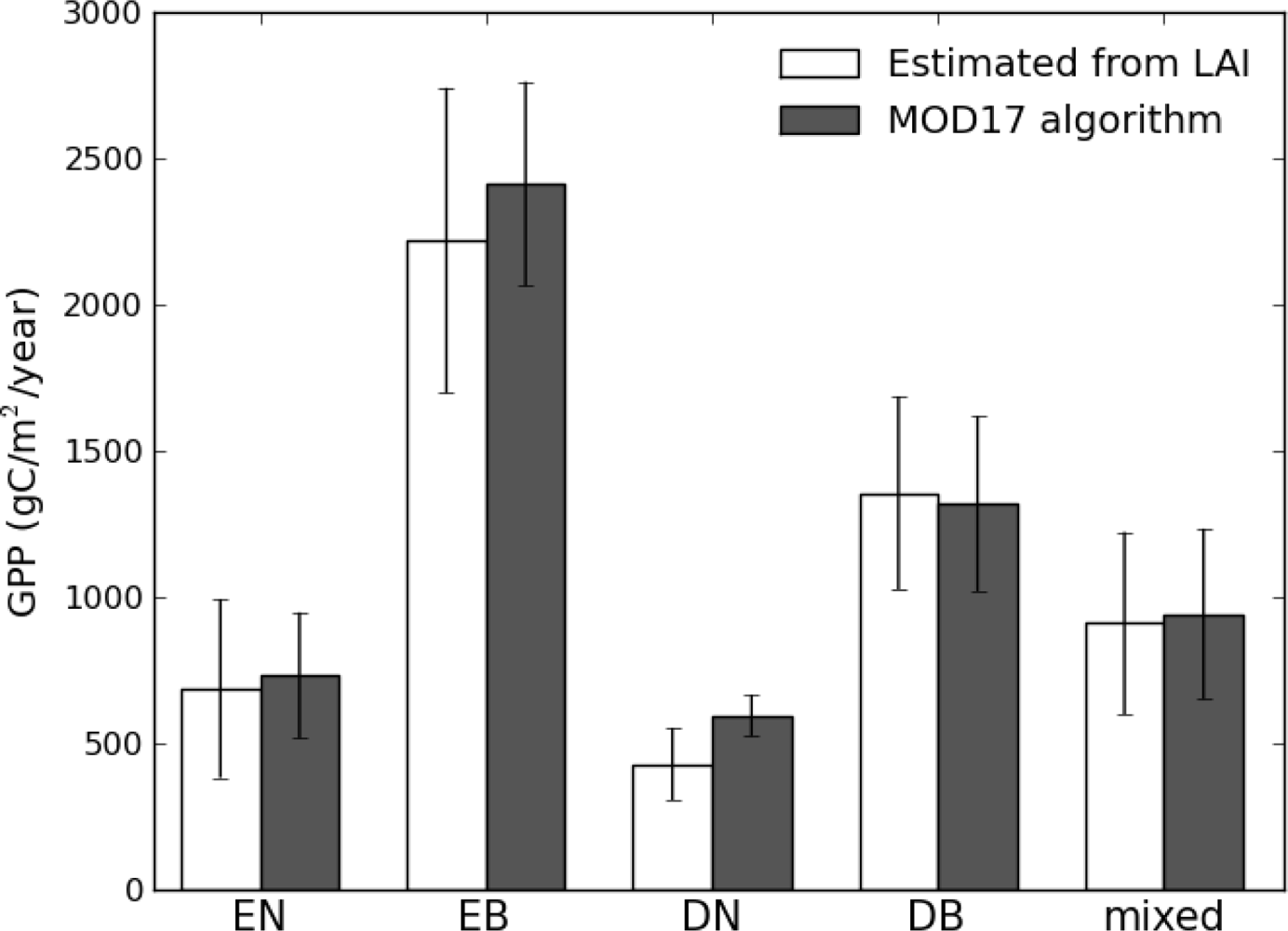
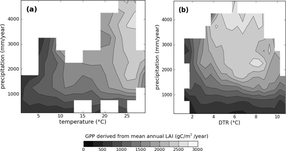
3.3. Assessment of the Simple GPP Model with MOD17 GPP and Climate

As a broader evaluation of the use of a simple approach to estimate annual GPP, we then applied equation 4 to MOD15 LAI product globally and compared it to MOD17 GPP (both subset for forested areas, aggregated to 0.5 degrees, and calculated as a 2001 to 2006 climatology). We used the monthly 0.25 degree Collection 5 MOD15 LAI product from Boston University [37] and 1 km global MOD17 Collection 5.1 annual GPP from the University of Montana [69]. We compared the single-metric GPP with MOD17 GPP for Evergreen Needleleaf Forest (ENF), Evergreen Broadleaf Forest (EBF), Deciduous Needleleaf Forest (DNF), Deciduous Broadleaf Forest (DBF), and mixed forest. Figure 6 shows that the best-performing single-product GPP model (Equation (4)) and the more complex MOD17 GPP produced comparable climatological GPP estimates with similar standard deviations, with the average LAI-based GPP (Equation (4)) only slightly lower than MOD17 GPP, except for deciduous broadleaf forest.
Finally, to assess whether our LAI-based GPP estimates were consistent with expectations relatively to climate, we plotted global annual GPP against mean temperature, annual precipitation, and mean diurnal temperature range (DTR) derived from the CRU TS 3.1 datasets. Our results for global forested areas show that the LAI-based GPP behaves as expected, with the highest values found in conditions of high temperature and precipitation and moderate DTR, while the lowest values are found in cold and dry climates (Figure 7).

4. Discussion

4.1. Why is Annual Mean LAI the Best Satellite-Derived Estimator of Annual GPP?

LAI showed the highest correlation with annual GPP among the satellite metrics presented in this study (Table 4). This strong connection between annual GPP and annual mean LAI has previously been documented through ground measurements by Kira et al. [70] and Waring et al. [71], who showed high correlations between GPP and Leaf Area Duration (LAD = growing season LAI × the number of growing season months). The relationship can be explained biophysically with the observation that larger canopies and longer growing seasons allow more carbon to be assimilated. Conversely, as more carbon is fixed as GPP, more carbon is allocated to leaf production. Although annual mean LAI correlates well with annual GPP, seasonal LAI correlates poorly with seasonal GPP because it does not respond to short term stresses such as anomalous heat waves.
The high correlation across different forest types can be explained by the functional convergence hypothesis [72]. The functional convergence hypothesis states that plants tailor their photosynthetic capacity to the amount of the most limiting resource so that optimal use is made of all resources [72]. The hypothesis has been well examined at the leaf level and is used to explain the convergence of leaf traits, such as the high correlation between photosynthetic capacity and leaf nitrogen content [73,74]. At the landscape or global level, the functional convergence hypothesis can be extended to explain the high correlation between absorbed PAR (APAR) and net primary production, and leads to assuming a constant LUE (Field, 1991). Goetz et al. [75] concluded that, because of the wide variability of carbon use efficiency (NPP/GPP), it is the LUE of GPP that should converge rather than the LUE of NPP. Since APAR is a function of LAI, the functional convergence theory should apply also for the relation between annually integrated GPP and LAI. Hence, we expect the annual GPP and LAD to be tightly correlated, even though over shorter time periods there can be a discrepancy between GPP and LAI, as shown in Table 3. Similar results were found when calculating GPP and LAI using prognostic ecosystem models [65].
Vegetation indices plots (Figure 3) showed non-linear relationship with GPP and a very different scatter from LAI plots (Figure 4). Vegetation indices do not monotonically increase with LAI mainly because of (1) canopy structural parameterization in the radiative transfer model of the MOD15 algorithm and (2) higher sensitivity of LAI to the reflectances in the saturation range of vegetation indices [35].

4.2. Why was the Performance of EVI Different between the Short-Term and Long-Term Spatial Analysis?

Our results suggest that simple models are viable approaches for estimating GPP, but that fundamentally different approaches should be used depending on the spatio-temporal scale of the analysis. Among the four satellite-derived metrics, EVI showed the highest correlation with short-term GPP (Table 3) but not with annual GPP (Table 4). The reason for the higher correlation of EVI than NDVI with short-term measurements of GPP can be attributed to (1) its broader dynamic range compared to NDVI, which is due to non-saturation at high LAI, (2) empirical auto-correction for atmospheric contamination of the reflectance, and (3) consistent retrievability without need of backup algorithms. Other studies also showed that EVI can track the seasonal change in GPP and other phenological events better than NDVI for deciduous forest [21].
However, when assessed at the level of either non-tropical or tropical sites to annual mean GPP, EVI had almost no correlation with annual GPP, while NDVI had significant correlation (Table 4). This result indicates that the conversion factor from EVI to GPP varies across forest types. That is not surprising considering that vegetation indices are a metric that is only theoretically proportional to leaf amount at any single point [76]. There is no clear biophysical justification for which the GPP/VI ratio should be constant among different biomes. Huete et al. [77] also reported that the slopes of the linear regression between monthly EVI and monthly GPP depended on biome type. In this study, the correlations between annual maximum VIs and annual maximum GPP were 0.47 (p < 0.001) for NDVI and 0.17 for EVI, indicating that the GPP/EVI ratio was site-specific rather than constant. This explains why annual mean EVI showed no correlation with annual GPP (Table 4).
To check if these results depended on the assumptions made for winter LAI in the presence of snow, and hence the calculation of the mean values, we set the value of the snow-covered pixels to the annual minimum rather than zero. While this increased the correlations of NDVI and EVI (R2 = 0.63 for NDVI and R2 = 0.62 for EVI), it did not significantly affect the correlation of LAI and FPAR. However, these results did not change how well those metrics were correlated because increases in the winter values proportionally increased the annual mean values. Thus, our results were not dependent on setting the snow values to zero.

4.3. Assessment of the LAI Empirical Relationship with Other Datasets

Our analysis shows that the simple model for estimating annual GPP from LAI has comparable accuracy—at global scales—to the MOD17 GPP product (Figure 6). LAI-based estimates are also consistent with the expected influence of climate on GPP (Figure 7), with estimates increasing with precipitation and temperature and average DTR. High DTR is indicative of dry conditions, while lower DTR is associated with low radiation. Both conditions are unfavorable for vegetation photosynthetic activity, as are extreme cold and low precipitation [78]. The fact that our GPP estimates broadly follow these patterns lends additional confidence that the simple approach does not generate spurious predictions. Our estimates of GPP for both tropical (2,332.9 g C/m2/year) and non-tropical (755.6 g C/m2/year) forest are also comparable to the ensemble median of 6 models by Beer et al. [2], further supporting that our results are reasonable.
At finer temporal resolutions, or for interannual variability, important differences may exist between the LAI-based GPP and MOD17, and we do not argue the two approaches are necessarily interchangeable. Indeed, in spite of errors and/or biases in input meteorology, upstream MODIS products, and structural issues with the algorithm itself [31,79], MOD17 is more highly correlated to the short-term measured GPP than any of the single MODIS products. But for research focused on broad-scale patterns of annual GPP variability, the simple model does appear to provide a useful alternative, and one that is consistent with theoretical principles developed decades ago.

4.4. Effects of Uncertainties in MODIS Products on Their Relationship with Annual GPP

In Section 2 we discussed the uncertainty introduced in the MODIS products by possible cloud contamination of the pixels and how to minimize it by temporally compositing the datasets.
In the case of MOD15, the propagation of algorithm uncertainties presents additional issues in the estimation of GPP. As described in Section 2.1, the algorithm uncertainty of LAI and FPAR was estimated through ground validation studies. Here, we assess the influence of MOD15 uncertainty on the GPP estimate through comparison with CYCLOPES [80], the other existing global LAI dataset. CYCLOPES LAI has a 1/112 degree spatial resolution and 10-day temporal sampling. The algorithm utilizes a neural network approach to retrieve LAI from SPOT VEGETATION reflectance data. We processed the CYCLOPES dataset to 30-day composites similarly to the MOD15 LAI 30-composites and calculated the correlation with annual GPP. In contrast to the high correlation between MODIS annual mean LAI and GPP, CYCLOPES annual mean LAI had an R2 of only 0.02 when compared to the annual flux tower GPP. Thus, annual GPP estimates appear to be sensitive to the uncertainty of the LAI products. The differences between MOD15 and CYCLOPES were mostly pertaining to: (a) Definition of LAI, with CYCLOPES measuring effective LAI while MODIS algorithm retrieves true LAI accounting for leaf clumping; (b) Nadir view TOA reflectances are input to the CYCLOPES LAI algorithm, while spectral surface reflectances with varying view angles are input into the MODIS algorithm; (c) Early saturation of the CYCLOPES LAI product, with maximum values limited to LAI = 4 while MODIS retrieves LAI of values up to 7 (includes both main algorithm and backup algorithm retrievals); (d) Classification errors due to differences in land cover mapping. These algorithm differences suggest caution when applying the proposed GPP estimation method to algorithm dataset different than MOD15.
Another potential source of uncertainty could be caused by the spatial resolution of the datasets. We used 250 m resolution data of MOD13, 1 km resolution data of MOD15 and MOD17, and flux tower point GPP data. We avoided the uncertainty caused by within-pixel spatial heterogeneity by applying a strict selective process to use only data for towers located over homogenous land covers, as described in Section 2. Also, Sims et al. [23] showed that comparisons between flux tower GPP and EVI were largely insensitive to the selection of a 3 km by 3 km grid versus a single 1 km pixel. Thus, we believe that our analysis was hardly affected by spatial resolution effects.
Unfortunately, the number of tropical forest flux sites was very small compared to boreal or temperate forest sites. In this study, we used 4 sites in South East Asia and 1 site in South America. More data for tropical forest are needed to improve the GPP estimation over these regions, likely altering the regression for the tropics.

5. Conclusions

We analyzed the correlation of MODIS NDVI, EVI, LAI and FPAR products with short-term and annual GPP measured at eddy covariance flux towers. Our results show that EVI is useful for the analysis of short-term variations in tower-estimated GPP (i.e., at the time scale of weeks to months) in agreement with other studies. Some diagnostic models started to utilize the EVI-GPP seasonal correlation, but caution should be exercised when mapping geographic patterns of GPP using EVI, because the EVI/GPP relationship is not constant across forest types. In our study, annual mean MODIS LAI was the best metric for estimation of the spatial patterns of annual GPP (GPP in g C/m2/year = 617 × LAI − 376). Annual mean NDVI and EVI were less correlated to tower-estimated GPP, but annual mean NDVI was a better predictor than annual mean EVI of annual GPP in non-tropical areas, suggesting that the GPP/EVI ratio is site specific. Extrapolating the relationship between annual mean LAI and annual GPP at the tower sites to forests globally produced reasonable GPP estimates that were also consistent with known climatic influences on GPP. The results allowed the rediscovery of the ground measured LAI and tower-estimated GPP relationship, as explained by strongly interrelated biophysical processes and the functional convergence hypothesis.
There are several concerns related to the uncertainty of MODIS products. These analyses were based on MODIS products, and different satellite products may be not able to get such high correlation between annual mean LAI and annual GPP. For the uncertainty caused by different resolution analysis, we minimized the influence on GPP estimate by carefully choosing the dataset not to include contaminated or heterogeneous data.

Acknowledgments

We sincerely appreciate the help of the researchers affiliated with the FLUXNET program. This study was funded by NASA’s Earth Sciences Program. We are grateful to Alessandro Cescatti and Scott Goetz for useful comments.

References and Notes

  1. Milesi, C.; Hashimoto, H.; Running, S.W.; Nemani, R.R. Climate variability, vegetation productivity and people at risk. Global Planet. Change 2005, 47, 221–231. [Google Scholar]
  2. Beer, C.; Reichstein, M.; Tomelleri, E.; Ciais, P.; Jung, M.; Carvalhais, N.; Rödenbeck, C.; Arain, M.A.; Baldocchi, D.; Bonan, G.B.; et al. Terrestrial gross carbon dioxide uptake: Global distribution and covariation with climate. Science 2010, 329, 834–838. [Google Scholar]
  3. Gholz, H.L. Environmental limits on aboveground net primary production, leaf area, and biomass in vegetation zones of the Pacific Northwest. Ecology 1982, 63, 469–481. [Google Scholar]
  4. Webb, W.L.; Lauenroth, W.K.; Szarek, S.R.; Kinerson, R.S. Primary production and abiotic controls in forests, grasslands, and desert ecosystems in the United States. Ecology 1983, 64, 134–151. [Google Scholar]
  5. Monteith, J.L. Solar radiation and productivity in tropical ecosystems. J. Appl. Ecol 1972, 9, 747–766. [Google Scholar]
  6. Goward, S.N.; Tucker, C.J.; Dye, D.G. North American vegetation patterns observed with the NOAA-7 Advanced Very High Resolution Radiometer. Plant Ecol 1985, 64, 3–14. [Google Scholar]
  7. Running, S.W.; Nemani, R.R. Relating seasonal patterns of the AVHRR vegetation index to simulated photosynthesis and transpiration of forests in different climates. Remote Sens. Environ 1988, 24, 347–367. [Google Scholar]
  8. Monteith, J.L. Climate and the efficiency of crop production in Britain. Phil. Trans. Roy. Soc. B 1977, 281, 277–294. [Google Scholar]
  9. Running, S.W.; Nemani, R.R.; Peterson, D.L.; Band, L.E.; Potts, D.F.; Pierce, L.L.; Spanner, M.A. Mapping regional forest evapotranspiration and photosynthesis by coupling satellite data with ecosystem simulation. Ecology 1989, 70, 1090–1101. [Google Scholar]
  10. Kato, T.; Tang, Y. Spatial variability and major controlling factors of CO2 sink strength in Asian terrestrial ecosystems: Evidence from eddy covariance data. Global Change Biol 2008, 14, 2333–2348. [Google Scholar]
  11. Wu, C.; Niu, Z.; Gao, S. Gross primary production estimation from MODIS data with vegetation index and photosynthetically active radiation in maize. J. Geophys. Res 2010, 115, D12127. [Google Scholar]
  12. Xiao, J.; Zhuang, Q.; Law, B.E.; Chen, J.; Baldocchi, D.D.; Cook, D.R.; Oren, R.; Richardson, A.D.; Wharton, S.; Ma, S.; et al. A continuous measure of gross primary production for the conterminous United States derived from MODIS and AmeriFlux data. Remote Sens. Environ 2010, 114, 576–591. [Google Scholar]
  13. Law, B.E.; Falge, E.; Gu, L.; Baldocchi, D.D.; Bakwin, P.; Berbigier, P.; Davis, K.; Dolman, A.J.; Falk, M.; Fuentes, J.D.; et al. Environmental controls over carbon dioxide and water vapor exchange of terrestrial vegetation. Agr. Forest Meteorol 2002, 113, 97–120. [Google Scholar]
  14. Tucker, C.J.; Townshend, J.R.G.; Goff, T.E. African land-cover classification using satellite data. Science 1985, 227, 369–375. [Google Scholar]
  15. Nemani, R.R.; Keeling, C.D.; Hashimoto, H.; Jolly, W.M.; Piper, S.C.; Tucker, C.J.; Myneni, R.B.; Running, S.W. Climate-driven increases in global terrestrial net primary production from 1982 to 1999. Science 2003, 300, 1560–1563. [Google Scholar]
  16. Gutman, G.G. On the use of long-term global data of land reflectances and vegetation indices derived from the Advanced Very High Resolution Radiometer. J. Geophys. Res 1999, 104, 6241–6255. [Google Scholar]
  17. Justice, C.O.; Vermote, E.; Townshend, J.R.G.; DeFries, R.; Roy, D.P.; Hall, D.K.; Salomonson, V.V.; Privette, J.L.; Riggs, G.; Strahler, A.; et al. The Moderate Resolution Imaging Spectroradiometer (MODIS): Land remote sensing for global change research. IEEE Trans. Geosci. Remote Sens 1998, 36, 1228–1249. [Google Scholar]
  18. Running, S.W.; Baldocchi, D.D.; Turner, D.P.; Gower, S.T.; Bakwin, P.S.; Hibbard, K.A. A global terrestrial monitoring network integrating tower fluxes, flask sampling, ecosystem modeling and EOS satellite data. Remote Sens. Environ 1999, 70, 108–127. [Google Scholar]
  19. Baldocchi, D.; Falge, E.; Gu, L.; Olson, R.; Hollinger, D.; Running, S.; Anthoni, P.; Bernhofer, C.; Davis, K.; Evans, R.; et al. FLUXNET: A new tool to study the temporal and spatial variability of ecosystem-scale carbon dioxide, water vapor, and energy flux densities. Bull. Am. Meteorol. Soc 2001, 82, 2415–2434. [Google Scholar]
  20. Huete, A.; Didan, K.; Miura, T.; Rodriguez, E.P.; Gao, X.; Ferreira, L.G. Overview of the radiometric and biophysical performance of the MODIS vegetation indices. Remote Sens. Environ 2002, 83, 195–213. [Google Scholar]
  21. Xiao, X.; Hollinger, D.; Aber, J.; Goltz, M.; Davidson, E.A.; Zhang, Q.; Moore, B., III. Satellite-based modeling of gross primary production in an evergreen needleleaf forest. Remote Sens. Environ 2004, 89, 519–534. [Google Scholar]
  22. Rahman, A.F.; Sims, D.A.; Cordova, V.D.; El-Masri, B.Z. Potential of MODIS EVI and surface temperature for directly estimating per-pixel ecosystem C fluxes. Geophys. Res. Lett 2005, 32, L19404. [Google Scholar]
  23. Sims, D.A.; Rahman, A.F.; Cordova, V.D.; El-Masri, B.Z.; Baldocchi, D.D.; Flanagan, L.B.; Goldstein, A.H.; Hollinger, D.Y.; Mission, L.; Monson, R.K.; et al. On the use of MODIS EVI to assess gross primary productivity of north American ecosystems. J. Geophys. Res 2006, 111, G04015. [Google Scholar]
  24. Huete, A.R.; Restrepo-Coupe, N.; Ratana, P.; Didan, K.; Saleska, S.R.; Ichii, K.; Panuthai, S.; Gamo, M. Multiple site tower flux and remote sensing comparisons of tropical forest dynamics in Monsoon Asia. Agr. Forest Meteorol 2008, 148, 748–760. [Google Scholar]
  25. Potter, C.; Klooster, S.; Huete, A.; Genovese, V. Terrestrial carbon sinks for the United States predicted from MODIS satellite data and ecosystem modeling. Earth Interact 2007, 11, 1–21. [Google Scholar]
  26. Sims, D.A.; Rahman, A.F.; Cordova, V.D.; El-Masri, B.Z.; Baldocchi, D.D.; Bolstad, P.V.; Flanagan, L.B.; Goldstein, A.H.; Hollinger, D.Y.; Misson, L.; et al. A new model of gross primary productivity for North American ecosystems based solely on the enhanced vegetation index and land surface temperature from MODIS. Remote Sens. Environ 2008, 112, 1633–1646. [Google Scholar]
  27. Wu, C.; Chen, J.M.; Huang, N. Predicting gross primary production from the enhanced vegetation index and photosynthetically active radiation: Evaluation and calibration. Remote Sens. Environ 2011, 115, 3424–3435. [Google Scholar]
  28. ORNL DAAC. MODIS Subsetted Land Products, Collection 5; ORNL DAAC: Oak Ridge, TN, USA, 2009. Available online: http://daac.ornl.gov/MODIS/modis.html from (accessed on 20 January 2012).
  29. Wolfe, R.E.; Nishihama, M.; Fleig, A.J.; Kuyper, J.A.; Roy, D.P.; Storey, J.C.; Patt, F.S. Achieving sub-pixel geolocation accuracy in support of MODIS land science. Remote Sens. Environ 2002, 83, 31–49. [Google Scholar]
  30. Myneni, R.B.; Hoffman, S.; Knyazikhin, Y.; Privette, J.L.; Glassy, J.; Tian, Y.; Wang, Y.; Song, X.; Zhang, Y.; Smith, G.R.; et al. Global products of vegetation leaf area and fraction absorbed PAR from year one of MODIS data. Remote Sens. Environ 2002, 83, 214–231. [Google Scholar]
  31. Zhao, M.; Heinsch, F.A.; Nemani, R.R.; Running, S.W. Improvements of the MODIS terrestrial gross and net primary production global data set. Remote Sens. Environ 2005, 95, 164–176. [Google Scholar]
  32. Holben, B.N. Characteristics of maximum-value composite images from temporal AVHRR data. Int. J. Remote Sens 1986, 7, 1417–1434. [Google Scholar]
  33. Tucker, C.J.; Fung, I.Y.; Keeling, C.D.; Gammon, R.H. Relationship between atmospheric CO2 variations and a satellite-derived vegetation index. Nature 1986, 319, 195–199. [Google Scholar]
  34. Myneni, R.B.; Keeling, C.D.; Tucker, C.J.; Asrar, G.; Nemani, R.R. Increased plant growth in the northern high latitudes from 1981 to 1991. Nature 1997, 386, 698–702. [Google Scholar]
  35. Yang, W.; Tan, B; Huang, D.; Rautiainen, M.; Shabanov, N.V.; Wang, Y.; Privette, J.L.; Huemmrich, K.F.; Fensholt, R.; Sandholt, I.; et al. MODIS Leaf Area Index Products: From validation to algorithm improvement. IEEE Trans. Geosci. Remote Sens 2006, 44, 1885–1898. [Google Scholar]
  36. Aragão, L.E.O.C.; Shimabukuro, Y.E.; Sabto, F.D.B.E.; Williams, M. Spatial validation of the collection 4 MODIS LAI product in Eastern Amazonia. IEEE Trans. Geosci. Remote Sens 2005, 43, 2526–2534. [Google Scholar]
  37. De Kauwe, M.G.; Disney, M.I.; Quaife, T.; Lewis, P.; Williams, M. An assessment of the MODIS collection 5 leaf area index product for a region of mixed coniferous forest. Remote Sens. Environ 2011, 115, 767–780. [Google Scholar]
  38. Ganguly, S.; Samanta, A.; Schull, M.A.; Shabanov, N.V.; Milesi, C.; Nemani, R.R.; Knyazikhin, Y.; Myneni, R.B. Generating vegetation leaf area index earth system data record from multiple sensors. Part 2: Implementation, analysis and validation. Remote Sens. Environ 2008, 112, 4318–4332. [Google Scholar]
  39. Heinsch, F.A.; Zhao, M.; Running, S.W.; Kimball, J.S.; Nemani, R.R.; Davis, K.J.; Bolstad, P.V.; Cook, B.D.; Desai, A.R.; Ricciuto, D.M.; et al. Evaluation of remote sensing based terrestrial productivity from MODIS using regional tower eddy flux network observations. IEEE Trans. Geosci. Remote Sens 2006, 44, 1908–1925. [Google Scholar]
  40. Atlas, R.M.; Lucchesi, R. File Specific for GEOS-DAS Gridded Output; Goddard Space Flight Center: Greenbelt, MD, USA, 2000. [Google Scholar]
  41. Reichstein, M.; Falge, E.; Baldocchi, D.; Papale, D.; Aubinet, M.; Berbigier, P.; Bernhofer, C.; Buchmann, N.; Gilmanov, T.; Granier, A.; et al. On the separation of net ecosystem exchange into assimilation and ecosystem respiration: Review and improved algorithm. Global Change Biol 2005, 11, 1424–1439. [Google Scholar]
  42. Papale, D.; Valentini, R. A new assessment of European forests carbon exchanges by eddy fluxes and artificial neural network spatialization. Global Change Biol 2003, 9, 525–535. [Google Scholar]
  43. Papale, D.; Reichstein, M.; Aubinet, M.; Canfora, E.; Bernhofer, C.; Kutsch, W.; Longdoz, B.; Rambal, S.; Valentini, R.; Vesala, T.; et al. Towards a standardized processing of Net Ecosystem Exchange measured with eddy covariance technique: Algorithms and uncertainty estimation. Biogeosciences 2006, 3, 571–583. [Google Scholar]
  44. Lasslop, G.; Reichstein, M.; Papale, D.; Richardson, A.D.; Arneth, A.; Barr, A.; Stoy, P.; Wohlfahrt, G. Separation of net ecosystem exchange into assimilation and respiration using a light response curve approach: Critical issues and global evaluation. Global Change Biol 2010, 16, 187–208. [Google Scholar]
  45. Turner, D.P.; Ritts, W.D.; Cohen, W.B.; Maeirsperger, T.K.; Gower, S.T.; Kirschbaum, A.A.; Running, S.W.; Zhao, M.; Wofsy, S.C.; Dunn, A.L.; et al. Site-level evaluation of satellite-based global terrestrial gross primary production and net primary production monitoring. Global Change Biol 2005, 11, 666–684. [Google Scholar]
  46. Hirata, R.; Saigusa, N.; Yamamoto, S.; Ohtani, Y.; Ide, R.; Asanuma, J.; Gamo, M.; Hirano, T.; Kondo, H.; Kosugi, Y.; et al. Spatial distribution of carbon balance in forest ecosystems across East Asia. Agr. Forest Meteorol 2008, 148, 761–775. [Google Scholar]
  47. Kutsch, W.L.; Kolle, O.; Rebmann, C.; Knohl, A.; Ziegler, W.; Schulze, E.-D. Advection and resulting CO2 exchange uncertainty in a tall forest in central Germany. Ecol. Appl 2008, 18, 1391–1405. [Google Scholar]
  48. Grünwald, T.; Bernhofer, C. A decade of carbon, water and energy flux measurements of an old spruce forest at the anchor station Tharandt. Tellus B 2007, 59, 387–396. [Google Scholar]
  49. Rebmann, C.; Zeri, M.; Lasslop, G.; Mund, M.; Kolle, O.; Schulze, E.-D.; Feigenwinter, C. Treatment and assessment of the CO2-exchange at a complex forest site in Thuringia, Germany. Agr. Forest Meteorol 2010, 150, 684–691. [Google Scholar]
  50. Chiesi, M.; Maselli, F.; Bindi, M.; Fibbi, L.; Cherubini, P.; Arlotta, E.; Tirone, G.; Matteucci, G.; Seufert, G. Modelling carbon budget of Mediterranean forests using ground and remote sensing measurements. Agr. Forest Meteorol 2005, 135, 22–34. [Google Scholar]
  51. Dolman, A.J.; Moors, E.J.; Elbers, J.A. The carbon uptake of a mid latitude pine forest growing on sandy soil. Agr. Forest Meteorol 2002, 111, 157–170. [Google Scholar]
  52. McMillan, A.M.S.; Goulden, M.L. Age-dependent variation in the biophysical properties of boreal forests. Global Biogeochem. Cy 2008, 22, GB2023. [Google Scholar]
  53. Davidson, E.A.; Richardson, A.D.; Savage, K.E.; Hollinger, D.Y. A distinct seasonal pattern of the ratio of soil respiration to total ecosystem respiration in a spruce-dominated forest. Global Change Biol 2006, 12, 230–239. [Google Scholar]
  54. Schmid, H.P.; Grimmond, C.S.B.; Cropley, F.; Offerle, B.; Su, H.-B. Measurements of CO2 and energy fluxes over a mixed hardwood forest in the mid-western United States. Agr. Forest Meteorol 2000, 103, 357–374. [Google Scholar]
  55. Gu, L.; Meyers, T.; Pallardy, S.G.; Hanson, P.J.; Yang, B.; Heuer, M.; Hosman, K.P.; Liu, Q.; Riggs, J.S.; Sluss, D.; et al. Influences of biomass heat and biochemical energy storages on the land surface fluxes and diurnal temperature range. J. Geophys. Res 2007, 117, D02107. [Google Scholar]
  56. Irvine, J.; Law, B.E.; Kurpius, M.R.; Anthoni, P.M.; Moore, D.; Schwarz, P.A. Age-related changes in ecosystem structure and function and effects on water and carbon exchange in ponderosa pine. Tree Physiol 2004, 24, 753–763. [Google Scholar]
  57. Domec, J.-C.; Noormets, A.; Sun, G.; King, J.; McNulty, S.; Gavazzi, M.; Boggs, J.; Treasure, E. Decoupling the influence of leaf and root hydraulic conductances on stomatal conductance and its sensitivity to vapour pressure deficit as soil dries in a drained loblolly pine plantation. Plant Cell Environ 2009, 32, 980–991. [Google Scholar]
  58. Monson, R.K.; Sparks, J.P.; Rosenstiel, T.N.; Scott-Denton, L.E.; Huxman, T.E.; Harley, P.C.; Turnipseed, A.A.; Burns, S.P.; Backlund, B.; Hu, J. Climatic influences on net ecosystem CO2 exchange during the transition from wintertime carbon source to springtime carbon sink in a high-elevation, subalpine forest. Oecologia 2005, 146, 130–147. [Google Scholar]
  59. Clark, K.L.; Gholz, H.L.; Castro, M.S. Carbon dynamics along a chronosequence of slash pine plantation in north Florida. Ecol. Appl 2004, 14, 1154–1171. [Google Scholar]
  60. Schmid, H.P.; Su, H.-B.; Vogel, C.S.; Curtis, P.S. Ecosystem-atmosphere exchange of carbon dioxide over a mixed hardwood forest in northern lower Michigan. J. Geophys. Res 2003, 108, 4417. [Google Scholar]
  61. Saleska, S.R.; Miller, S.D.; Matross, D.M.; Goulden, M.L.; Wofsy, S.C.; da Rocha, H.R.; de Camargo, P.B.; Crill, P.; Daube, B.C.; de Freitas, H.C.; et al. Carbon in Amazon forests: Unexpected seasonal fluxes and disturbance-induced losses. Science 2003, 302, 1554–1557. [Google Scholar]
  62. Hirano, T.; Segah, H.; Harada, T.; Limin, S.; June, T.; Hirata, R.; Osaki, M. Carbon dioxide balance of a tropical peat swamp forest in Kalimantan, Indonesia. Global Change Biol 2007, 13, 412–425. [Google Scholar]
  63. Mitchell, T.D.; Jones, P.D. An improved method of constructing a database of monthly climate observations and associated high-resolution grids. Int. J. Climatol 2005, 25, 693–712. [Google Scholar]
  64. Friedl, M.A.; McIver, D.K.; Hodges, J.C.F.; Zhang, X.Y.; Muchoney, D.; Strahler, A.H.; Woodcock, C.E.; Gopal, S.; Schneider, A.; Cooper, A.; et al. Global land cover mapping from MODIS: Algorithms and early results. Remote Sens. Environ 2002, 83, 287–302. [Google Scholar]
  65. Wang, W.; Dungun, J.; Hashimoto, H.; Michaelis, A.R.; Milesi, C.; Ichii, K.; Nemani, R.R. Diagnosing and assessing uncertainties of terrestrial ecosystem models in a multi-model ensemble experiment: 1. Primary production. Global Change Biol 2011, 17, 1350–1366. [Google Scholar]
  66. Sokal, R.R.; Rohlf, F.J. Biometry: The Principles and Practice of Statistics in Biological Research, 3rd ed.; W. H. Freeman and Company: New York, NY, USA, 1995. [Google Scholar]
  67. Turner, D.P.; Ritts, W.D.; Cohen, W.B.; Gower, S.T.; Stith, T.; Running, S.W.; Zhao, M.; Costa, M.H.; Kirschbaum, A.A.; Ham, J.M.; et al. Evaluation of MODIS NPP and GPP products across multiple biomes. Remote Sens. Environ 2006, 102, 282–292. [Google Scholar]
  68. Sellers, P.J. Canopy reflectance, photosynthesis and transpiration. Int. J. Remote Sens 1985, 6, 1335–1372. [Google Scholar]
  69. Numerical Terradynamic Simulation Group. Enhanced 1 km Global 8-day MODIS GPP/NPP (MOD17). 2009. Available online: ftp://ftp.ntsg.umt.edu/pub/MODIS/Mirror/MOD17A2.LATEST (accessed on 19 January 2012).
  70. Kira, T.; Shidei, T. Primary production and turnover of organic matter in different forest ecosystems of the Western Pacific. Ecol. Soc. Japan 1967, 17, 70–87. [Google Scholar]
  71. Waring, R.H.; Schlesinger, W.H. Forest Ecosystems: Concepts and Management; Academic Press: Orlando, FL, USA, 1985. [Google Scholar]
  72. Field, C.B. Ecological scaling of carbon gain to stress and resource availability. In Response of Plants to Multiple Stresses; Mooney, H.A., Winner, W.E., Pell, E.J., Eds.; Academic Press: San Diego, CA, USA, 1991; pp. 35–65. [Google Scholar]
  73. Reich, P.B.; Walters, M.B.; Ellsworth, D.S. From tropics to tundra: Global convergence in plant functioning. Proc. Natl. Acad. Sci. USA 1997, 94, 13730–13734. [Google Scholar]
  74. Wright, I.J.; Reich, P.B.; Westoby, M.; Ackerly, D.D.; Baruch, Z.; Bongers, F.; Cavender-Bares, J.; Chapin, T.; Cornelissen, J.H.C.; Diemer, M.; et al. The worldwide leaf economics spectrum. Nature 2004, 428, 821–827. [Google Scholar]
  75. Goetz, S.J.; Prince, S.D. Modelling terrestrial carbon exchange and storage: evidence and implications of functional convergence in light-use efficiency. Adv. Ecol. Res 1999, 28, 57–92. [Google Scholar]
  76. Myneni, R.B.; Nemani, R.R.; Running, S.W. Estimation of global leaf area index and adsorbed PAR using radiative transfer models. IEEE Trans. Geosci. Remote Sens 1997, 35, 1380–1393. [Google Scholar]
  77. Huete, A.R.; Didan, K.; Shimabukuro, Y.E.; Ratana, P.; Saleska, S.R.; Hutyra, L.R.; Yang, W.; Nemani, R.R.; Myneni, R. Amazon rainforests green-up with sunlight in dry season. Geophys. Res. Lett 2006, 33, L06405. [Google Scholar]
  78. Zhou, L.; Dai, A.; Dai, Y.; Vose, R.S.; Zou, C.; Tian, Y.; Chen, H. Spatial dependence of diurnal temperature range trends on precipitation from 1950 to 2004. Clim. Dynam 2009, 32, 429–440. [Google Scholar]
  79. Zhao, M.; Running, S.W.; Nemani, R.R. Sensitivity of Moderate Resolution Imaging Spectroradiometer (MODIS) terrestrial primary production to the accuracy of meteorological reanalyses. J. Geophys. Res 2006, D111, G01002. [Google Scholar]
  80. Baret, F.; Hagolle, O.; Geiger, B.; Bicheron, P.; Miras, B.; Huc, M.; Berthelot, B.; Niño, F.; Weiss, M.; Samain, O.; et al. LAI, fAPAR and fCover CYCLOPES global products derived from VEGETATION. Part 1: Principles of the algorithm. Remote Sens. Environ 2007, 110, 305–316. [Google Scholar]
Figure 1. Map of the flux tower sites used in this study. The data are from AmeriFlux in North America (1), CarboEurope in Europe (2), AmeriFlux in Brazil (3) and AsiaFlux in the Southeast Asia (4). Temperate deciduous forests are marked with gray symbols. Tropical forests are marked with white symbols.
Remotesensing 04 00303f1
Figure 2. Scatterplots of flux tower sites over the global climatology contour plot in the temperature-precipitation domain. The temperature and precipitation of flux towers are averaged measured values in the years when gross primary production (GPP) is available for analysis. The temperature and precipitation of the global climatology were calculated using Climate Research Unit (CRU) datasets from 1982 to 2009 base years. The contour are area-weighted histogram and the units of the color scale is km2/(1 °C)/(1 mm) bins. Only forested areas were plotted (as identified by MCD12C1 IGBP classification land cover data).
Remotesensing 04 00303f2
Figure 3. Scatterplot of 32-day composites of GPP vs. (a) Normalized Difference Vegetation Index (NDVI), (b) Enhanced Vegetation Index (EVI), (c) Leaf Area Index (LAI), and (d) Fraction of Photosynthetically Active Radiation (FPAR) using data from all the sites.
Remotesensing 04 00303f3
Figure 4. Scatterplot of annual mean MOD13 NDVI (a) and EVI (b) against flux tower annual GPP. NDVI and EVI data were processed to a 32-day maximum value composite (MVC) before calculating the annual mean value. The solid line represents the reduced major axis regression between the variables. The dashed lines are 95% confidence interval lines. Multiple points for a given site correspond to data from different years.
Remotesensing 04 00303f4
Figure 5. Scatterplot of annual mean MOD15 LAI (a) and FPAR (b) against flux tower annual GPP. LAI and FPAR were processed to a 32-day maximum value composite (MVC) before calculating the annual mean value. The solid line represents the reduced major axis regression between the variables. The dashed lines are 95% confidence interval lines.
Remotesensing 04 00303f5
Figure 6. Average and standard deviation of estimated LAI-based and MOD17 annual GPP for each forest type: Evergreen Needleleaf Forest (EN), Evergreen Broadleaf Forest (EB), Deciduous Needleleaf Forest (DN), Deciduous Broadleaf Forest (DB), and mixed forest. The statistics are calculated from all the available 0.5-degree pixels grouped by forest type using the MODIS Land Cover MCD12C1 V005 IGBP classification scheme data.
Remotesensing 04 00303f6
Figure 7. Contour plots of estimated GPP against temperature and precipitation (a) and against precipitation and diurnal temperature range (DTR) (b).
Remotesensing 04 00303f7
Table 1. Description of Moderate Resolution Imaging Spectroradiometer (MODIS) product subsets.
ProductsSpatial ResolutionCompositing PeriodCitation
MOD13Q1NDVI and EVI250 m16 dayHuete et al. [20]
MOD15A2LAI and FPAR1 km8 dayMyneni et al. [30]
MOD17A2GPP/NPP1 km8 dayZhao et al. [31]
Table 2. Site description of flux towers used in this study. Forest types are: deciduous broad leaf forest (DB), evergreen needleleaf forest (EN), and evergreen broad leaf forest (EB). Note that the years given in the table refer to the available data before applying the criteria described in Sections 2.1 and 2.2, and thus the actual number of years used in the analysis may be smaller.
Site NameAbbreviationCountry/StateLatitude (°N)Longitude (°E)Forest TypeYearCitation
Non-tropicsHainichDE-HaiGermany51.07910.452DB2001–2007Kutsch et al. [47]
TharandtDE-ThaGermany50.96413.567EN2001–2003Grünwald et al. [48]
WetzsteinDE-WetGermany50.45411.458EN2002–2008Rebmann et al. [49]
San RossoreIT-SRoItaly43.73010.287EN2001–2004Chiesi et al. [50]
LoobosNL-LooNetherlands52.1685.744EN2001–2008Dolman et al. [51]
UCI-1964 burn siteCA-NS3Canada55.912−98.382EN2001–2005McMillan et al. [52]
UCI-1989 burn siteCA-NS6Canada55.917−98.964EN2001–2005McMillan et al. [52]
Howland Forest (west tower)US-Ho2Maine, US45.209−68.747EN2001–2004Davidson et al. [53]
Morgan Monroe State ForestUS-MMSIndiana, US39.323−86.413DB2001–2006Schmid et al. [54]
Missouri OzarkUS-MOzMissouri, US38.744−92.200DB2004–2006Gu et al. [55]
Metolius Intermediate PineUS-Me2Oregon, US44.452−121.557EN2002–2007Irvine et al. [56]
Metolius First Young PineUS-Me5Oregon, US44.437−121.567EN2001–2002Irvine et al. [56]
North Carolina Loblolly PineUS-NC2North Carolina, US35.803−76.668EN2005–2006Domec et al. [57]
Niwot Ridge ForestUS-NR1Colorado, US40.033−105.546EN2001–2007Monson et al. [58]
MizeUS-SP2Florida, US29.765−82.245EN2001–2004Clark et al. [59]
Univ. of Mich. Biological StationUS-UMBMichigan, US45.560−84.714DB2001–2006Schmid et al. [60]
TropicsSantarem Km83 Logged ForestBR-Sa3Brazil−3.018−54.971EB2001–2003Saleska et al. [61]
Bukit SoehartoID-BukIndonesia-0.833117.050EB2002Huete et al. [24]
PalangkarayaID-PalIndonesia−2.345114.036EB2002–2003Hirano et al. [62]
Mae KlongTH-MaeThailand14.57598.858DB2003–2004Huete et al. [24]
SakaeratTH-SakThailand14.493101.922EB2002–2003Huete et al. [24]
Table 3. Average R2 between each MODIS product and flux tower GPP for each composite period. The values in parenthesis are root mean square error (RMSE; gC/m2/day) calculated by reduced major axis regression analysis. Average R2 and RMSE are the average of all the R2 and RMSE calculated from each year of each site, respectively. n is number of sites used for the calculations.
Composite PeriodAll (n = 21)Deciduous (n = 5)Evergreen (n = 16)Non-Tropical (n = 16)Tropical (n = 5)
MOD13NDVI16-day0.44 (2.08)0.64 (2.36)0.38 (1.98)0.51 (2.14)0.13 (1.78)
32-day0.47 (1.94)0.65 (2.31)0.41 (1.80)0.54 (2.00)0.16 (1.68)

EVI16-day0.55 (1.70)0.78 (1.73)0.47 (1.69)0.64 (1.70)0.11 (1.67)
32-day0.54 (1.67)0.77 (1.80)0.46 (1.62)0.62 (1.72)0.20 (1.42)

MOD15LAI8-day0.38 (2.21)0.60 (2.56)0.30 (2.08)0.44 (2.31)0.13 (1.82)
16-day0.43 (1.86)0.69 (2.05)0.34 (2.02)0.50 (2.09)0.13 (1.75)
32-day0.51 (1.70)0.69 (2.09)0.38 (1.77)0.56 (1.89)0.10 (1.72)

FPAR8-day0.31 (2.42)0.54 (2.81)0.23 (2.28)0.35 (2.57)0.14 (1.81)
16-day0.36 (2.26)0.62 (2.45)0.27 (2.20)0.41 (2.37)0.12 (1.77)
32-day0.40 (1.90)0.62 (2.38)0.33 (1.91)0.47 (2.19)0.12 (1.63)

MOD17GPP8-day0.68 (1.31)0.72 (1.95)0.67 (1.11)0.82 (1.17)0.12 (1.91)
Table 4. Summary of R2 between each MODIS product and flux tower annual GPP. The stars indicate p-value < 0.05 (*) and p-value < 0.001 (**).
Composite PeriodAll SitesNon-Tropical SitesTropical Sites
MOD13NDVI16-day0.50**0.48**0.30
32-day0.57**0.42**0.32

EVI16-day0.56**0.010.01
32-day0.54**0.010.11

MOD15LAI8-day0.78**0.43**0.70*
16-day0.83**0.57**0.68*
32-day0.88**0.68**0.66*

FPAR8-day0.56**0.46**0.64*
16-day0.58**0.59**0.55*
32-day0.62**0.63**0.57*

MOD17GPP8-day0.81**0.59**0.01

