Enhancing Coral Health Detection Using Spectral Diversity Indices from WorldView-2 Imagery and Machine Learners

USR 3278 CRIOBE CNRS-EPHE, BP 1013, Papetoai, Moorea 98729, French Polynesia
*
Author to whom correspondence should be addressed.
Remote Sens. 2012, 4(10), 3244-3264; https://doi.org/10.3390/rs4103244
Submission received: 16 August 2012
/
Revised: 9 October 2012
/
Accepted: 12 October 2012
/
Published: 23 October 2012
Abstract
:The worldwide waning health of coral reefs implies an increasing need for monitoring them at colony scale over large areas. Relaying fieldwork considerably, the remote sensing approach can address this need in offering spectral information relevant for coral health detection with 0.5 m spatial accuracy. We investigated the potential of spectral diversity indices to achieve the discrimination of coral-dominated assemblages and health states from novel satellite imagery (WorldView-2, WV2). Both Equitability’s (E) and Pielou’s (P) operators were used to quantify the evenness of the corrected visible spectral bands (two times 26 combinations of five bands) corresponding to remotely sensed colonies. Three scleractinian corals (Porites lobata, P. rus and Acropora pulchra) that are primarily involved in Moorea’s reef building (French Polynesia) were examined in respect to their health state (healthy or unhealthy, referring to both bleached and dead coral, hereinafter). Using four classifiers, we showed that the Support Vector Machine (SVM) greatly discerned among the six coral classes based upon the five WV2 spectral bands (93%), thus surpassing the classification issued from the three traditionally used bands (80%). Coupling the WV2 dataset with Egreen-red, Eyellow-red or E“coastal”-blue-green allowed the SVM performance to attain 96%. On the other hand, adding the E“coastal”-blue to the WV2-dataset contributed to a substantially increase of the classification accuracy derived from the Random Forest classifier, stepping from 64% to 77%. Significant contributions of spectral diversity indices to surveying coral health were further discussed in the light of spectral properties of coral-related pigments. These findings may play a major role for the extensive monitoring of coral health states at a fine scale, and for the management and restoration of damaged coral reefs.

1. Introduction
Coral ecosystems worldwide were estimated to provide US$ 375 billion worth of ecological services, such as disturbance regulation, food production or cultural goods [1]. However, these marine biodiversity hotspots are increasingly undermined by a wealth of stressors, ranging from the global sea level and temperature rising [2] to ocean acidification impairing the calcification rate [3] through increased frequency of tropical cyclone events [4]. In addition, global climate change intensifies local stresses including disease, overfishing, sedimentation and chemical pollution related to anthropogenic activities [5] leading to a loss of biodiversity at an unprecedented rate during the Anthropocene. Since ecosystem functioning and subsequent services are recognized to be tightly correlated with biodiversity [6], the rapid shrinkage of scleractinian corals (reef builders) harboring a large amount of marine species will entail the collapse of the coral ecosystems driving humans toward a costly restoration. The characterization of the reef builders’ health is therefore required to reliably assess the coral ecosystems’ evolution and further take decisive action to manage them.
Coral reef monitoring is traditionally completed by field campaigns, which are highly time-consuming. The need to adopt survey alternatives to evaluate the diversity of scleractinian corals at colony scale (i.e., ∼0.5 to 2 m) over large extents (i.e., tens to hundreds km) has prompted an increasing use of optical remote sensing imagery [7,8]. Over the last decade, advances in coral reef remote sensing have enabled the mapping of coral reef geomorphology [9], benthic cover [10], and notably observation of coral bleaching [8,11]. Focused on either the spatial or spectral issues, researchers have raised specific questions and successfully addressed them in fully exploiting their capabilities. Coral-related benthic habitat classification was therefore underpinned both by the enhancement of the spatial resolution of multispectral spaceborne sensors leading to the 2.4 m QuickBird-2 [12], and by the increase in the spectral bands for hyperspectral airborne sensors resulting in the 512 band Airborne Imaging Spectroradiometer for Applications [13]. The multispectral spaceborne imagery was able to rapidly span tens of hundreds km of coral reefs, but was limited by the restricted number of broad spectral bands. Despite the improvement dedicated to the spatial resolution, the broad-colored vision restrains the definition of a coral colony in terms of discrete function due to low separability power between spectral signatures. The spaceborne sensors have gradually become specific and even compelling for studies of reef geomorphology and benthic mapping discriminating coarse level classes, such as corals, macroalgae and sand. The hyperspectral airborne (or even handborne) imagery can distinguish among main coral species and between healthy and bleached corals when measured with narrow spectral bands, i.e., 10–20 nm [14–16]. While strongly dependent on favorable environmental conditions and restricted to local scale surveys, hyperspectral imagery has increasingly been used for spectrally accurate benthic mapping confined to areas of interest less than several km2 in size, allowing a medium to fine level discrimination.
The spaceborne WorldView-2 (WV2) sensor, launched in October 2009, provides eight bands at 2 m spatial resolution, that is to say twice the spectral capabilities of its predecessor, QuickBird-2 (Table 1). The WV2 imagery has proven to be able to increase separability between land and shallow water ecotopes [17]. Through the acquisition of five water-transmitted spectral bands at a 0.5 m-pansharpened pixel size, WV2 holds great promise to bridge the spatio-spectral accuracy of airborne sensors and the large-scale coverage of spaceborne instruments. However, prior to achieve the bridge, we need to overcome the limitations inherent to the bandwidths, remaining relatively broad to ensure a high signal-to-noise ratio, that is to say for compensating for light absorption and scattering, occurring both in atmosphere and hydrosphere. Since only severely bleached coral can be identified by hyperspectral derivative spectroscopy [14,16] with high accuracy, we develop hereinafter an innovative classification methodology based on diversity indices [18] applied to coral spectral signatures so that distinction between healthy and unhealthy states, more subtle than bleached states, can be completed.
This study aims to examine whether the very high spatial and enhanced spectral resolution of WV2 imagery is able to distinguish between two health states of three tropical reef builders. The limited seabed classes considered in this study are useful as a first step toward a full evaluation of WV2 imagery for monitoring coral health. Specific purposes to be reached are (1) to show that the spectral signatures of the main reef builders Porites lobata, P. rus and Acropora pulchra are discernable using both the WV2 novel band combination and four state-of-the-art machine learners, (2) to evaluate whether the spectral signatures of healthy and unhealthy corals are distinguishable, (3) to determine whether the spectral diversity indices such as Equitability’s (E) and Pielou’s (P) evenness contributes to substantial enhancement in coral discrimination, and (4) to map the most contributing spectral diversity index compounded with the best classification
2. Methodology
2.1. Study Site
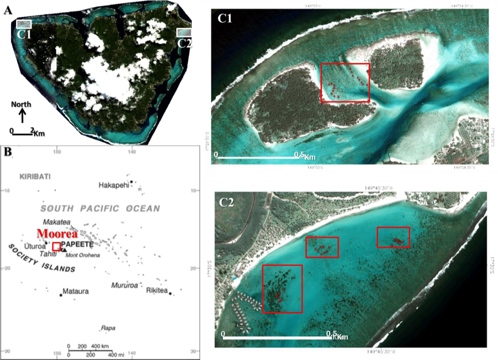
The study was undertaken at two sites in the lagoon of Moorea island (17°29′31″S, 149°50′08″W) in the Society Archipelago, French Polynesia (Figure 1). Remote tropical islands in Pacific Ocean are particularly suited for coastal remote sensing because of the high visibility of the water column and the relatively high coral cover (>30%) in the shallow lagoon part. Due to these characteristics, it is important to bear in mind that this study is context-specific and confined to the shallow lagoon part of Pacific coral reefs. The first site (Between Motu) was situated in the northwestern lagoon within the Tiahura Marine Protected Area (MPA). This area benefits from a 40-year-old monitoring of coral reef ecology. Specifically, the site consists of a shallow water area surrounded by two vegetated emerged reef flats, called motu. This site was selected based upon the large size of Porites sp. stony colonies, the variety of their health state and the ease of watercraft access. Large colonies (ranging from 1 to 9.25 m2) allowed the spectral mixing to be minimized in providing a sufficient amount of pansharpened pixels (ranging from 4 to 37) to ensure statistically robust spectral signatures. The low average (image-derived) depth, i.e., 0.46 ± 0.05 m, was an advantage to correctly position the watercraft installed with a GPS despite the strong current velocity. The second site (Temae), located in the northeastern lagoon within Nuarai MPA, is characterized by a vast shallow water area punctuated by massive Porites sp. stony colonies (from 1 to 10 m2) and extended Acropora pulchra fields (from 4.25 to 337.5 m2). The site runs alongside a coralline sand shore and has an average depth of 3.15 ±0.46 m.
2.2. Ground-Truthing
In order to link the WV2 imagery with bathymetry and seabed measurements, in situ ground-truthing was acquired for model calibration and validation. Even if the fieldwork was carried out in 26–27 June 2010, no major event such as tropical cyclone or outbreak of corallivore predators (e.g., crown-of-thorne sea star, Acanthaster planci) occurred since the date of image acquisition. Regarding bathymetry, a 0.1 m accuracy acoustic system (sonar Lowrance LMS-527C DF iGPS) was used to measure water depths at the two sites. The acoustic system was set up on a 5 m aluminum boat designed for lagoon fieldwork. Each acoustic measurement was collected while a nadir angle, indicated by a weighted rope, was positioned lower than 10°. The geo-positioning was ensured by a 0.5 m horizontal accuracy Trimble GPS Geo XH. The datum employed was WGS-84 and the projection referenced to UTM Zone 6 South. As for the seabed survey, nine 0.5 m × 0.5 m quadrats per station (N = 40, Figure 1(C1 and C2)) were set up over the colonies examined in the two sites. A 2 × 10⁻⁴ m accuracy photograph, using a hand-held Panasonic DMC-TS2, and GPS coordinates were taken for each quadrat. The quadrat frame constituted the planar referential aiming at correcting the perspective induced by the photograph angle. The GPS antenna, mounted on a vertical 3 m bar, was centered on the quadrat. Between Motu and Temae, sites were all composed of 360 quadrat-pixels.
2.3. Image Processing
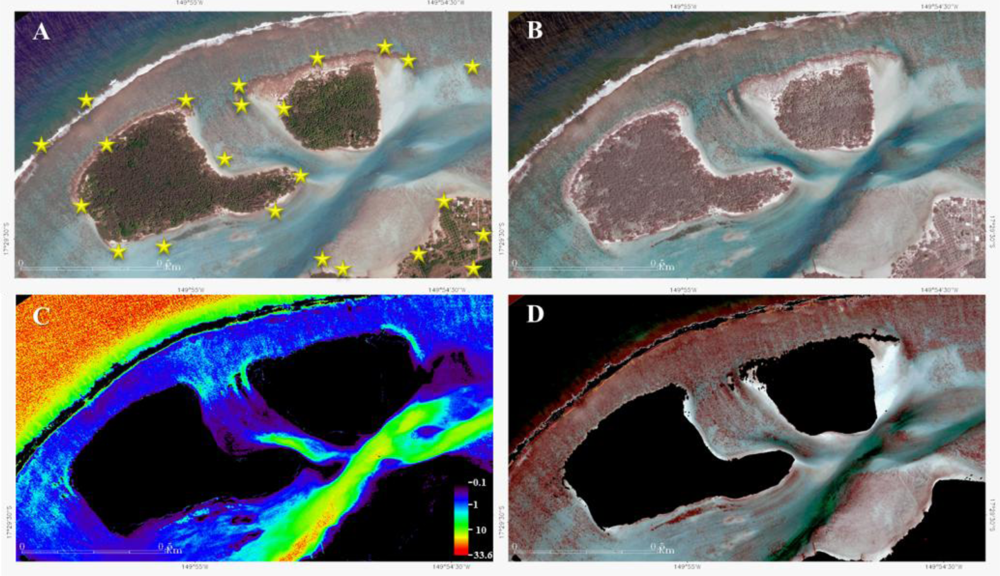
Two WorldView-2 (WV2) datasets were used in this study: the first was acquired on 12 February 2010 and the second was collected on 17 March 2010. Each dataset consisted of a 2 m multispectral image (eight bands) and a 0.5 m panchromatic image with their respective metadata files. The WV2 multispectral mode monitored five visible and three Near InfraRed (NIR) bands (Table 1) with an 11-bit radiometric accuracy. Over the two sites, no water cloud or particle plume impeded the scene, and both water surface and clarity were suited for seafloor analyses. A glint-removal procedure was therefore unnecessary. Prior to novel analysis inherent to this study, a procedure was applied to correct each of the two images using IDL-ENVI software (Research Systems, Inc., Boulder, CO, USA). First, geometric correction was carried out using the parameters describing the sensor-scene geometry (contained in the .rpb file), and in situ geolocations of features easily recognizable on the imagery (23 for the Between Motu site in Figure 2(A) and 37 for the Temae site), called ground control points (GCP). A second order polynomial warping model was used so that low complex non-linear distortions could be corrected. For each study area, we retained only the combination of GCP associated with a Root Mean Square Error (RMSE) less than or equal to 0.5 m. The nearest-neighbor interpolation applied to the resampling allowed data values to be conserved without averaging. Second, radiometric correction was divided into radiance calibration and atmosphere correction. The radiance calibration (in W·m−2·sr−1) was achieved by computing the at-sensor radiance in multiplying digital numbers by coefficients recorded in the .imd file (see Between Motu site, Figure 2(A)). The atmosphere correction was completed by parameterizing the MODTRAN4 algorithm, core of the Fast Line-of-site Atmospheric Analysis of Spectral Hypercubes (FLAASH) module, with the acquisition metadata. In addition to accounting for absorption and scattering occurring in the air column over marine tropical zones, the algorithm corrected for adjacency effects (see Between Motu site, Figure 2(B)). The atmosphere-corrected dataset was expressed in the form of reflectance, i.e., unitless as ratio between water-leaving radiance and downwelling irradiance entering the water. Once previous the steps were completed for both multispectral and panchromatic images, the pansharpening procedure was carried out to scale up the spatial resolution of the multispectral dataset using the component substitution method [19]. The further selection of the simulation and resampling methods was a crucial step aiming at mediating spectral changes between initial and pansharpened images. We therefore used the sensor sensitivity and the cubic convolution for the fusion of the multispectral 2 m resolution image with the panchromatic 0.5 m resolution image, resulting in a multispectral 0.5 m resolution [20]. The sensor sensitivity method builds the simulated panchromatic image as the weighted combination of all multispectral bands.
The light direction and transmission are strongly affected by interactions in the water column. The change of optical medium (from air to water) is related to a change in light direction as a function of the refractive index (cf. Descartes’ law), dependent on temperature and salinity. The radiation propagation is then altered by interactions with water molecules, dissolved and particle matter. Interactions such as diffusion and absorption entail an exponential decay in radiance (or reflectance) in respect to water column height. Lyzenga [21] demonstrated that relationships relating the reflectance, at one waveband, to the water depth and the benthic (bottom) albedo could be modeled as follows:
where Rw refers to the reflectance above the water surface, R∞ is the water reflectance while the water column is optically deep (typically > 40 m depth) in order to circumvent the bias due to the benthic-associated reflectance component. Ab is the benthic albedo, Kd is the diffuse attenuation coefficient, and Z is the actual depth.
Attempting to process data without correction of bathymetry-induced attenuation can lead to a dramatic confusion between benthic features. Spectral signatures of reef builders can be confounded and those of their health state cannot be disentangled. Traditional methods for compensating for attenuation effects of variable depth on benthic radiance relied on the method derived by Lyzenga [21,22]. Although this method was commonly adopted, the estimation of depth (using two bands) needed to determine five variables empirically. The tuning of the variables raised issues either for the inherent intensive fieldwork or, conversely, for the assumed unrealistic homogeneity of parameters. An alternative solution requiring only one parameter to adjust was proposed by Stumpf et al. [23] and defined the bathymetry Z as follows:
where Rwi and Rwj refer to reflectance above the water surface of “coastal” and green wavebands [24], respectively, m1 is the adjustable function allowing the ratio to be depth-scaled, n is a fixed constant ensuring that the logarithm will be positive, and m0 is the offset.
The adjustable function m1 was determined using 166 bathymetric soundings collected from the 0.1 m accuracy acoustic system. The relationship between ratio values and ground-truth soundings was satisfactorily modeled by an exponential function (R2 = 0.7328):
The calibration equation was implemented, and site-attached Triangular Irregular Networks (TIN) were linearly interpolated to build two 0.5 m Digital Depth Models (DDM) (Figure 2(C)). The maximum depth attained was 33.6 m, while the minimum depth was 0.12 m, corresponding to the vertical resolution of the DDM. A set of 34 bathymetric soundings was used to validate the model. A satisfactory agreement between DDM and validation soundings was computed (R2 = 0.84). Since the validation points did not span all the bathymetric variability (e.g., deep water), the value of the maximum depth has to be cautiously considered.
The knowledge of the water depth is required to quantify the loss of light in the water column, to thereafter compensate for this amount of light, and lastly to elucidate the benthic albedo. By inverting the radiative transfer model (Equation (1)), the benthic albedo (Ab) can be expressed as follows:
The diffuse attenuation coefficient, Kd, was estimated for each visible waveband by extracting the values from a previous study of optical properties of Moorea’s lagoon waters [25] (Table 2). Moorea’s waters basically fell into the oceanic case 1 water, where the concentration of chlorophyll and pheopigments is higher than the concentration of non-biogenic materials [26]. Although the last two bands displayed higher Kd than the first three bands, the use of the five-band dataset could be considered to be acceptable up to a six-meter depth [27].
Given (1) the water surface reflectance, (2) the estimates of both the water reflectance with no benthic influence, (3) the creation of the DDM, and (4) the values of the diffuse attenuation coefficient, the benthic albedo was solved (Figure 2(D)) for the entire scene.
2.4. Patterns of Coral Spectra
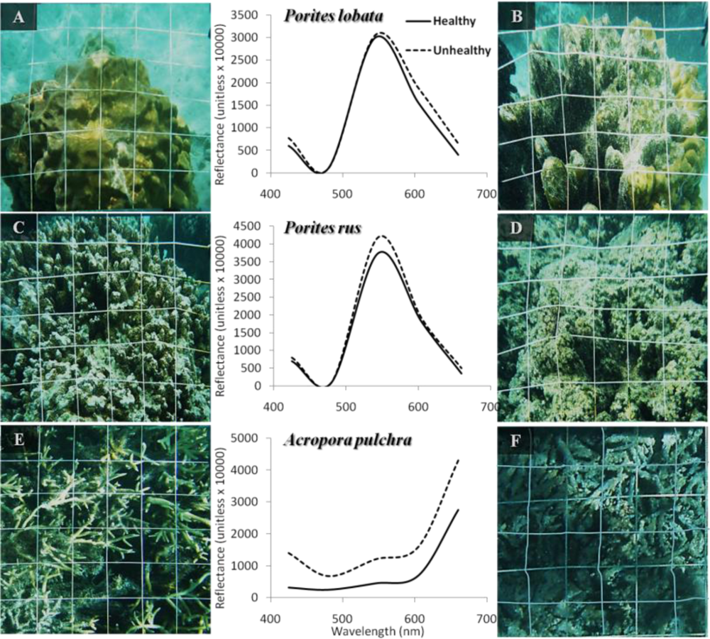
Corals examined for this study could be divided into two categories given their morphology and the spatial scale adopted: discrete massive boulders and continuous fields of branching corals. The first category encompassed the Hump Coral (Porites lobata) (Figure 3(A,B)) and the Finger Coral (Porites rus) (Figure 3(C,D)), while the second category was represented by the Staghorn Coral (Acropora pulchra) (Figure 3(E,F)). For each coral species, we focused on two health states, i.e., healthy and unhealthy, corresponding, respectively, to the sixth brightness-saturation and the grouping of the fifth-fourth-third-second-first brightness-saturation levels of the graduation established in the Coral Health Chart [28]. This tool refers to the colorfulness of coral-algal pigmentation and describes how the colors change as corals lose their symbionts. Each of the six classes (Figure 3) was defined in the form of its spectral signature in the five corrected WV2 visible bands.
2.5. Spectral Diversity Indices
Rapid assessment of coral health state is supported by visual examination of the surficial cover of the colony. While brightness and saturation of a colony radiant with health display low and high values in visible bands (i.e., live colors), respectively, those of an unhealthy colony show higher and lower values, respectively (i.e., drab colors or even dead colors referred to in American English) [28]. On the other hand, even though unhealthy corals (or bleached corals) usually display greater levels of brightness, some colonies can be colonized by turf algae that absorb light, thus enhancing the saturation of the underlying coral structure. The comparison of reflectance can therefore be confined to a specific subset depending on both imagery correction and local environmental conditions. Through the computation of band frequency (relative abundance), the spectral diversity ensures (1) the comparison between spectra to be stable over various locations, and (2) bands involved in the detection of coral health state to be identified.
A spectral diversity index is a mathematical measure, which is intended to measure the relative distribution of an array of wavebands. This index basically provides statistical information about predominance and evenness of bands in a spectrum. The ability to quantify reflectance diversity contributes to support the understanding of spectrum structure related to coral-dominated assemblages and health states. From the diversity indices commonly employed in ecology, we selected two: the Equitability’s (E) and the Pielou’s (P) evenness indices. While the E index is based on the Simpson index [29], the P index refers to as the Shannon-Weaver entropy function [30]. E was computed as follows:
where n is the number of bands, and pi is the relative contribution of the ith band within the whole spectrum. P is defined as follows:
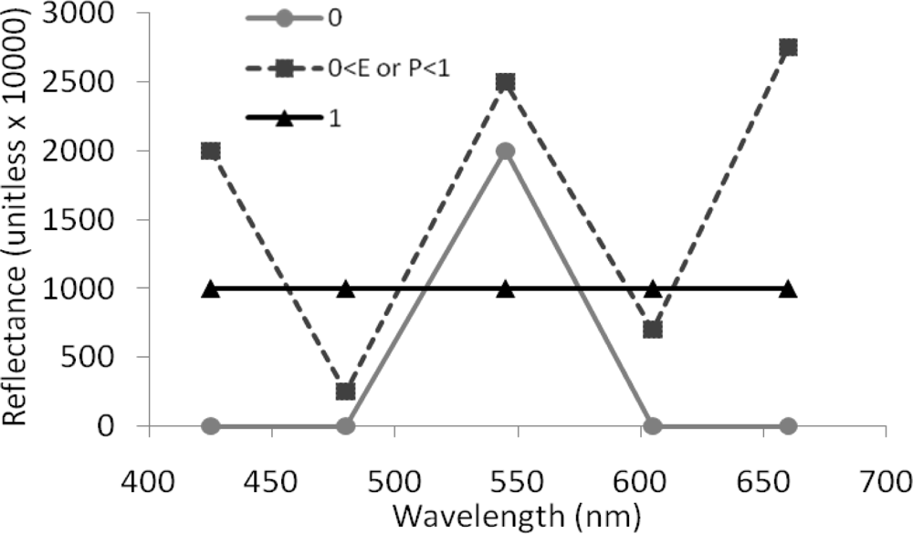
Both indices returned a value of zero if the spectrum was characterized by a unique band and rose to one in cases where the spectrum showed strict equivalent proportions for all bands (Figure 4). A greater diversity of wavebands increased E and P values. While the theoretical computation of the E index derived from the product of the proportions, the computation of the P index relied on the product of the proportions and the logarithmic product. When a dominance related to a band occurs, the E index should be lower than the P index.
A multispectral approach was adopted to evaluate the information gain conveyed by both diversity indices. For each spectral diversity index (E and P), a series of 26 band combinations was computed as a result of the sum of the five-, four-, three-, and two-combination of the spectral set composed of five visible bands (n). More formally, it corresponds to the sum of the binomial coefficients:
Note, for instance, that the E index involving the combination of the five bands is denoted E12345, and the E index based on the combination of the “coastal” and blue bands is denoted E12 (cf. Table 1 for band numbering). This exhaustive analysis aimed at outlining the bands as well as the combinations of bands that substantially contribute to the improvement of the discrimination of the targeted corals. The implementation of the diversity indices was undertaken in the signal and image processing software IDL-ENVI (Research Systems, Inc., Boulder, CO, USA).
2.6. Classification
The classification procedure sought for discriminating both coral-dominated assemblages and health states using state-of-the-art learners. The pixels associated to the six classes (depicted in Figure 3) were extracted in the five visible bands, the 26 E and P indices. These ground-truth pixels were mixed across the two sites for the sake of representativeness and subsequently partitioned into two groups: a group intending for the learner training (2/3 pixels), and a group for model validation (1/3 pixels). Each of the six classes was represented by 40 training and 20 validation pixels. Four machine learners were selected as classifiers given their power of discrimination evidenced in recent studies [31,32]. Supervised learners can recognize complex blueprints that underlie relationships between the coral response variable and spectral explanatory variables. The ability to elucidate non-linear relationships allows those learners to mostly outperform traditionally used linear models [33]. Classification performances of Naïve Bayes (NB), k-Nearest Neighbour (kNN), Random Forest (RF) and Support Vector Machine (SVM) were examined in respect to the conventional three visible bands (QB2), the finely corrected five visible bands (WV2), the 26 E index-enhanced WV2 and the 26 P index-enhanced WV2. The NB is a simple probabilistic classifier based on applying Bayes’ theorem with strong independence assumptions. The kNN uses a function based on closest training samples in the feature space. The RF builds a set of classification trees that is composed of leaves representing predicted outcomes and branches representing conjunctions of features that lead to those outcomes [34]. The SVM constructs a separating hyperplane or set of hyperplanes in the variable-dimensioned space, which has the largest distance to the nearest samples of different classes. We highly recommend readers interested in parameterization and mathematical implications of those four algorithms to refer the paragraph dedicated to them in [32]. Prediction accuracy of the coral response stemming from the four learners was assessed by the validation dataset across the Classification Accuracy (CA) [35]. As a summary evaluator, the CA computed the ratio of the number of samples correctly classified divided by the total number of sample cases. Inspecting the class-level contribution of the various combinations of diversity indices to the WV2 dataset required to compute the Confusion Matrix (CM) that was created only for the best-fitted models. Models were developed and tested using the open-source Orange software [36].
3. Results and Discussion
The cogency of our results and discussion lay in the assumption that remotely-sensed spectra associated to the six coral-dominated classes were correlated with the spectral specificities of their pigments. This assumption stemmed from results of previous studies suggesting that benthic cover could be accurately mapped using remotely-sensed key wavelengths [37].
3.1. Increasing Spectral Bands Involved a Better Discrimination of Coral-Dominated Assemblages and Health State
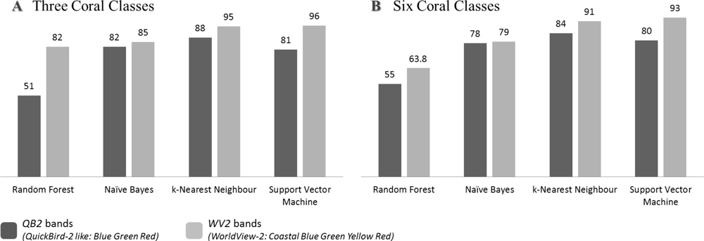
Irrespective of their health state, the three coral-dominated assemblages were correctly classified (CA > 80%) by the three spectral bands (QB2) for three out of four classifiers (Figure 5(A)). Although the RF showed a very moderate performance (CA = 51%), results inherent to the three other models all exceeded 80%. When developed from the five spectral bands (WV2), the CA consistently provided higher values, ranging from 82% to 96%, stemming from the RF and the SVM algorithms, respectively. These results demonstrated the interspecific spectral variability of corals that could be quantified even with only red, green and blue predictors. However, the addition of two spectral bands, i.e., “coastal” and yellow, allowed for an increase in the power of discrimination of the three coral-dominated assemblages.
Comparing both spectral datasets’ performances revealed that the WV2 dataset systematically outperformed the QB2 dataset against the four classifiers for distinguishing health states of the three coral-dominated assemblages (Figure 5(B)). Three out of the four algorithms (i.e., RF, kNN and SVM) showed that the value added of two bands was significant in terms of classification performance (pZ-test < 0.01,). As for the NB algorithm, albeit superior, no substantial contribution of the two added bands was detected (pZ-test = 0.018). While RF, NB, SVM and kNN gradually improved the QB2-derived classification, the RF, NB, kNN and SVM gradually refined the WV2-derived coral separation. Developing a model trained by three spectral bands for coral classification provided satisfactory results when using the kNN classifier (CA = 84%). On the other hand, analyzing coral spectra through five visible spectral bands rated the kNN and SVM to provide the best discernments (CA = 91%, and CA = 93%, respectively). This latter classifier incidentally displayed the highest difference between WV2 and QB2.
Classifying the health states of corals (i.e., six classes) resulted in a loss of the classification performance compared to classifying only the coral-dominated assemblages (i.e., three classes). Using the QB2 dataset, a reduction in CA, albeit slight (topped at 4%), appeared for the four classifiers. When employing the WV2 dataset, the decline in CA was slight for SVM, kNN and NB (2%, 4% and 6%, respectively) but exacerbated for RF (i.e., 18%). Irrespective of the number of spectral bands included in the classification scheme, scaling up the ecological accuracy in partitioning the coral-dominated assemblages as a function of their health states involved a decrease of the distinction, corroborating theory that underlies image classification.
Both the coral-dominated assemblages and their health states (healthy or unhealthy) were successfully predicted from multispectral remote sensing, even though the optical properties of the water column were assumed to remain homogeneous across the two study areas. Quadrat sampling was deliberately collected at different water depths, ranging from approximately 0.5 to 3 m, so that pattern recognition of coral-dominated assemblages and health state was not skewed by spectral changes induced by variation of depths. However, comparing spectra retrieved from sharply contrasted water depths (e.g., 0.5 vs. 20 m) and clarities (varying on short a distance in reef slope) could raise substantial issues when considering the diffuse attenuation coefficient, Kd, as constant over the lagoon. Expressed in the form of an exponential (Equation (1)), constant Kd could lead to strong discrepancies between water-corrected and actual reflectance in over- or under- estimating attenuation of the light in the water column (corresponding to a lower or higher in situ Kd, respectively). The problem of Kd assessment could be addressed, at least partially, by means of quantifying water clarity and pigment concentration during the field survey [38]. As it would be fragmented and time-consuming, such a survey could not bring enough information to be included in reef health monitoring procedure, demanding a high time/area ratio. Remote sensing of coral-dominated assemblages and health state will attain expectations of multi-scale managers and decision-makers as soon as the Kd can be resolved directly from the spaceborne imagery, as it can be done from the hyperspectral airborne imagery [39]. Recent applications of the spaceborne sensor QB2 [12] are very promising to retrieve the coefficient for each pixel and will be applied to fine-tune the WV2 radiative transfer model.
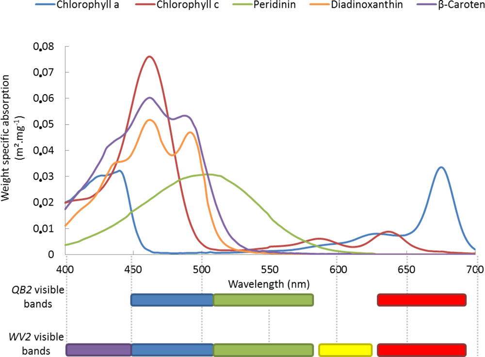
Adding the “coastal” and yellow bands to spectral variables underpinned that the WV2, as a very high spatial and enhanced spectral resolution spaceborne sensor, has the spectral capability to discriminate the ma or reef builder’s types at the colony scale (Figure 6 and [40]). Coral colors are recognized to be closely linked with absorption related to zooxanthellae (dinoflagellate endosymbiont of scleractinian corals). Examining the absorption spectrum of “brown” corals modeled by concentration-weighted pigments included in endosymbiotic zooxanthellae [41] pointed out that, while (1) conventional blue, green and red bands adequately recorded the last (i.e., third) peak of chlorophyll-a, the first peak, the start of the second peak and the end of the third peak of chlorophyll-c, the peak of the peridinin, the second and the third peaks of diadinoxanthin, as well as the second and the third peaks of β-caroten, (2) the “coastal” and the yellow bands allowed the first and the second peaks of chlorophyll-a, the second and third peak of chlorophyll-c, the first peak of diadinoxanthin, and the first peak of β-caroten to be detected. The spectral continuity conveyed by the adjacency of “coastal” and blue bands ensured the coverage of the first peak of chlorophyll-c, the spectrum of diadinoxanthin and of β-caroten. The association of the “coastal”, blue and green bands offered the complete detection of peridinin. The addition of the yellow and red bands enabled the sensing of both chlorophylls (i.e., their last two peaks). The specific contribution of the bands or combinations of bands to presence/absence coral-associated pigments will be further discussed in the light of spectral indices in the next section. Increasing the spectral resolution of a very high spatial resolution sensor encouraged the thought that this new tool would favorably enhance classification of coral reefs’ features, spanning other reef builders (e.g., Pocillopora sp., Montipora sp.), algae (macroalgae and coralline red algae), as well as sediment classes (mud, sand and reef flat) [20].
3.2. Spectral Diversity Indices Enhanced Classification of Coral-Dominated Assemblages and Health State
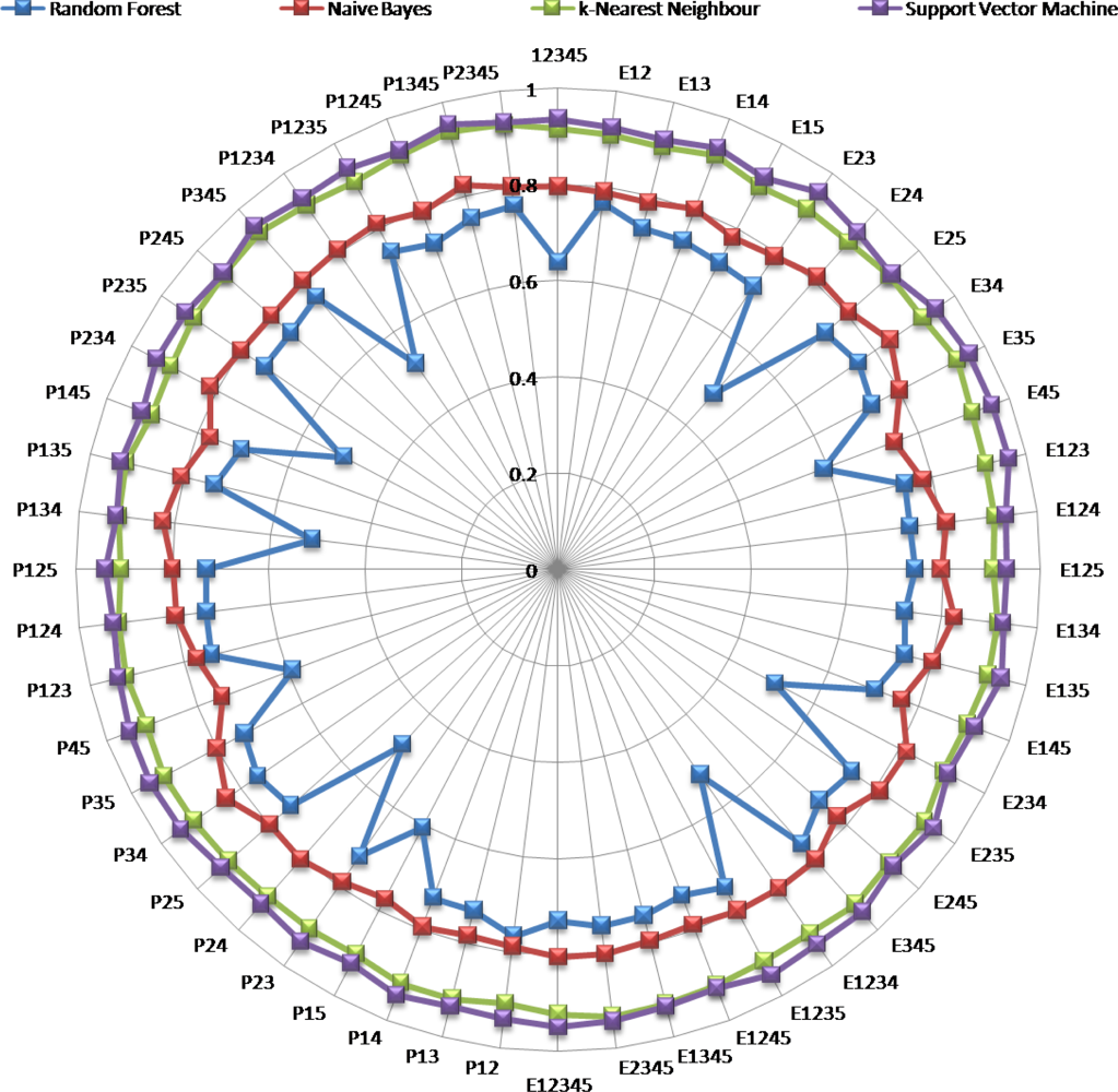
Beyond the efficient distinction of coral-dominated assemblages and health state retrieved from the original WV2 dataset, classifications modeled by the diversity index-boosted WV2 datasets produced high CA for all classifiers except RF (Figure 7). The “dart board-like” Figure 7 synoptically plotted 52 classification performances resulted from diversity index-enhanced WV2 combinations as a function of the four classifiers while remaining readable. At first sight, a hierarchy between classifiers, consistent across spectral combinations, could be outlined. Showing the lowest CA in the entire analysis (i.e., 49%), the RF embodied the worst classifier, followed by the NB, whose lowest value reached 75%, followed by the kNN and SVM, whose lowest values were close to 90%. According to this classifier’s sorting (from RF to SVM), the amplitude between the highest and the lowest CA for each classifier tended to diminish (namely, 28, 9, 4 and 5%, respectively), as visually represented by the circle linearity (Figure 7). Through distributions of the four circles against the CA gradient, two clusters emerged on either side of a numerical gap: The first group composed of the SVM and kNN was characterized by high and stable results, the second group encompassing the NB and the RF produced moderate and variable accuracies. CA appeared close enough to those issued from the WV2 dataset so that in-depth analyses regarding changes were conducted.
The contributions of both series of diversity indices brought distinctness among the coral classes to be refined despite the counter-intuitive negative contributions somewhat disseminated across the spectral combinations. While the best contribution for the RF occurred with E12 and P12 (gain of 13%), contributions of E24 and P24 substantially lowered the classification (loss of 15%). As for the NB, kNN and SVM, contributions of both best and worst diversity indices, albeit significant, were further reduced (gains of 4, 2 and 3%; losses of 5, 2 and 2%, respectively). While the best contributions for the NB, kNN and SVM stemmed from E34 and P34; E35, E2345, P345 and P1345; E35, E45 and E123, respectively, the worst contributions resulted from E45 and P45; E15; E234, respectively. Given the multiple similar contributions, we chose to further analyze the highest gain (i.e., RF) and the highest CA (i.e., SVM).
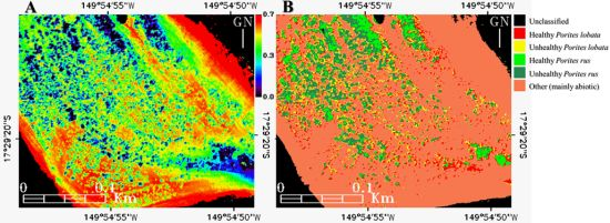
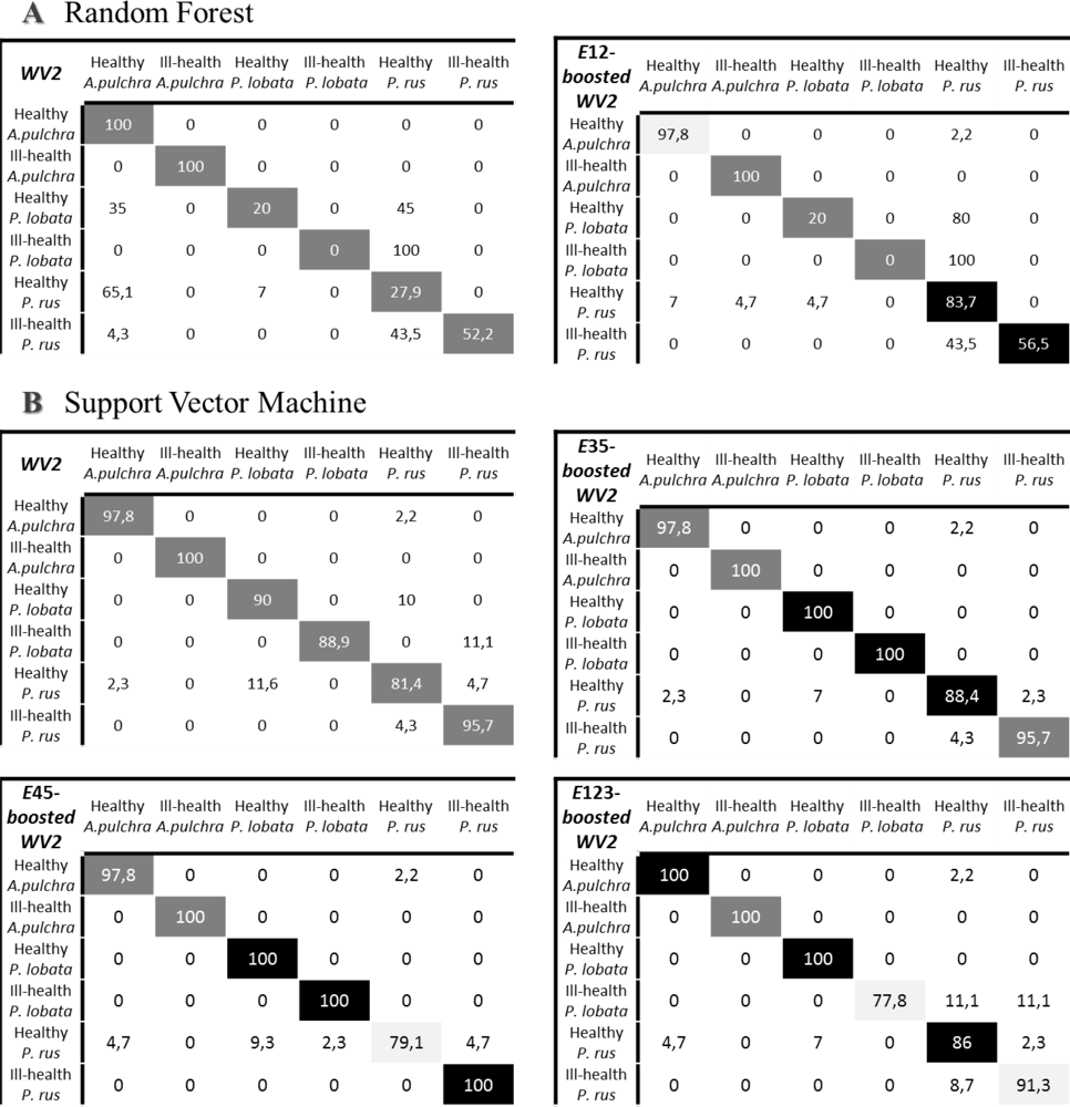
Changes in CA issued from the contribution of the best spectral indices were analyzed using confusion matrices (CM), allowing for the change detection at the class level. Despite the lowest CA among the four classifiers, the RF showed the highest gain using either the E12 or the P12. We could deduce that the knowledge of both “coastal” and blue reflectance could substantially enhance the discrimination among coral-dominated assemblages and health states. Confronting the CM derived from the WV2 and the E12-enhanced WV2 (CM of P12 was identical) datasets led to emphasize gains of both healthy P. rus (55.8%) and unhealthy P. rus (4.3%), as well as a slight loss of A. pulchra (2.2%) (Figure 8(A)). Although the diversity index-related gain was not huge, the SVM produced the best CA using the E35, the E45 and the E123. Retrieving the changes from the CM, we could infer that the index based upon (1) the green and the red reflectance refined distinction among healthy P. lobata (10%), unhealthy P. lobata (11.1%) and healthy P. rus (7%), (2) the yellow and the red reflectance augmented the CA of healthy P. lobata (10%), unhealthy P. lobata (11.1%), unhealthy P. rus (4.3%) at the expense of the healthy P. rus (2.3%), (3) the “coastal”, the blue and the green bands increased the CA of healthy A. pulchra (2.2%), healthy P. lobata (10%), healthy P. rus (4.6%) at the expense of unhealthy P. lobata (11.1%) and unhealthy P. rus (4.4%) (Figure 8(B)). CA of P. lobata derived from the SVM WV2 CM approximated those computed from an airborne 1 m spectrographic imager [42]. However, when boosted by E35, E45, E123, the CA equaled 100%, surpassing the airborne survey by around 10%. Compared to CA dedicated to remote sensing of (1) acroporid assemblages by a spaceborne multispectral 4 m sensor [43] and (2) an Acropora dataset by an in situ hyperspectral spectrometer [16], a gain of 10% occurred with and without E contribution. This finding proved the greater power of classification of the SVM algorithm vis à vis traditional classifiers used in those studies. We furthermore mapped the E123 index compounded with the E123-enhanced SVM classification (Figure 8(B)) of the first subregion (Figure 9) to demonstrate that our proof-of-concept was able to furnish meaningful information intelligible to marine spatial planners and lagoon practitioners.
The two series of spectral indices, i.e., E and P, differentially modified CA in respect to the classifiers. While the contribution’s differences between E and P negated 16 times (out of 26 possible) for the RF classifier, only five cases were reported for the SVM. Conversely, the maximum contribution difference topped at 0.21 and 0.02 for RF and SVM, respectively. The P index, computed on the basis of Shannon-Weaver entropy [29], weighed each band according to the attendant fraction of the whole measured light, that is to say, the frequency. On the other hand, the E index, based upon the Simpson index [29], attached much importance to the most dominant band since it involved the sum of the squares of the frequencies (note that the square of a small frequency was a very small number). We could deduce that (1) the E index tended to be lower than the P index when a band dominated, and (2) the greater the dominance in the spectrum, the greater the difference between these two indices. Across the four classifiers, the four worst and least bad contributions were found for the P series, while the E series contained the seven worst and four least bad contributions. In the light of previous theoretical findings, the prevalence of E in terms of highest absolute values of contribution indicated that the most significant spectral indices were more sensitive to spectral dominance. The corollary of this stronger sensitivity indicated that infrequent bands hardly contributed to the E indices. One way around this dilemma would be to use Hill’s diversity index, merging both previous diversity indices, allowing for a sharper view of the spectral diversity. While providing the measurement of the dominant bands, it would have the ability to incorporate the infrequent bands.
Comparing the spectral indices involved in the best contributions with the spectra of pigments including coral tissues highlighted spectral windows as valuable to discern between healthy and unhealthy corals (Table 3). The diversity index E12 provided the highest contribution to the RF in specifically increasing recognition of both health states of P. rus. This result suitably matched a spectroscopic study showing that the spectral region comprised between 430 and 490 nm displayed the highest differentiation among various health states of corals [16]. The absorption of the first peaks of chlorophyll-a and -c, diadinoxanthin and β-caroten were encompassed by the oint “coastal” and blue bands, ranging from 400 to 510 nm. We could therefore hypothesize that the four latter pigments were found to be relevant predictors of P. rus health state. Assuming that the absorption magnitude of these pigments responded to the zooxanthella density and that the zooxanthella density differed remarkably among various P.rus health states, the intensity of the remotely sensed reflectance between 400 and 510 nm would accurately measure the zooxanthella density, thus reflect the gradient of the P. rus health state. Beyond the binary classification of the health state (healthy and unhealthy), intermediate states would be inferred, offering a time flexibility, favorable to managing coral reefs. The diversity index E123 improved the SVM classification in gradually increasing healthy A. pulchra, P. rus and P. lobata at the expense of unhealthy P. rus and unhealthy P. lobata. Adding the green band to the previous diversity index pushed detection boundaries to 580 nm, thus integrating the peridinin into pigments detection (the four latter ones). While adding the peridinin detection led to slight misclassifications towards unhealthy corals, it augmented the detection of the healthy state of the three coral-dominated assemblages. These findings concurred with those of Clark et al. [44], showing a good discrimination of healthy and unhealthy coral in the 515–596 nm range. The slight misclassifications akin to unhealthy P. rus and unhealthy P. lobata might be explained by the presence of turf algae on colonies (e.g., Figure 3(B)). The within-pixel mixing of living and bleached coral tissue with algae cover is very susceptible to alter the spectral signature of a pure dead or bleached coral (deprived of pigment-related absorption per se) by diminishing the reflectance due to the chlorophyll-related absorption. The diversity index E35, involving the green and red bands, enabled the two health states of P. lobata and the healthy P. rus to be clearly separated. The monitoring of the second half of the peridinin spectrum and the last peak (the third) of chlorophyll-a could be deemed as meaningful for assessing P. lobata health state. The diversity index E45, bringing into play yellow and red bands, led to a better distinction among the two health states of P. lobata and the unhealthy P. rus. The adjacency of the two bands ensured the two last peaks (the second and third) of chlorophyll-a and -c to be fully covered. The knowledge of the red band, associated with either the green or yellow band, therefore suggested an enhancement in distinctness of P. lobata state health. Whereas the red band unequivocally fitted with last peak of chlorophyll-a, strong attenuation of the inherent radiation by water hindered its use for discriminating coral health state below a few meters depth (>4–5 m). In addition, when combined with green, red highlighted the healthy P. rus, while it emphasized the unhealthy P. rus with yellow. The presence of peridinin appeared decisive for the assessment of healthy P. rus, while the sensing of the two last peaks of cholorophyll-c suggested P. rus with poor health. This latter conclusion corroborated results derived from in situ spectroscopy analysis, specifying that spectral signature (reflectance) of worldwide-averaged “brown” corals was clearly characterized by a “triple-peaked pattern” ranging from 560 to 660 nm [15]. It is not possible to speculate on the spectral partitioning of the diversity index in the present study, but work is in progress to validate or refute previous inferences based upon assemblage of pigment spectra.
4. Conclusions
Remote sensing of tropical coral reefs has just taken a leap in matching very high spatial and visible multispectral resolution. First, the so-called “coastal” band, covering the purple spectrum, provided innovative measurements of light attenuation in air and water, from which accurate bathymetry (R2 = 0.84) was retrieved. Second, the properly corrected five visible bands offered a great discriminating power (93%) of the three main scleractinian corals in respect to their health state (healthy or unhealthy). Increasing the classification accuracy derived from the three visible bands QB2 sensor by 13%, the spaceborne WV2 sensor equaled spectroscopy-induced capabilities of airborne remote sensing [13–16], despite a coarser spectral resolution.
Coupling the WV2 dataset with spectral diversity indices, such as Egreen-red, Eyellow-red or E“coastal”-blue-green, enabled the SVM’s classification performance to attain 96%. On the other hand, adding the E“coastal”-blue to the WV2-dataset contributed to a substantial increase of the classification accuracy derived from the Random Forest (RF), stepping from 64% to 77%. In the light of spectral properties of pigments included in coral tissues, we identified patterns matching spectral diversity indices with coral-dominated assemblages. While E“coastal”-blue favored discrimination of P. rus, E“coastal”-blue-green better discerned among the three species (P. rus, P. lobata and A. pulchra), Egreen-red and Eyellow-red enhanced distinction of P. lobata. Our premise is that spectral diversity indices were, for this work, a surrogate for diagnosing coral vitality and morbidity with the assumptions that the spectral contamination towards coral-dominated assemblages was insignificant and that the density of coral-attached pigments was correlated with coral health. These findings, once validated in an entire scene with other benthic classes, are likely to help understand phase shifts from complex to degraded coral ecosystems, and have profound implications for management and restoration of these marine hotspots.
Acknowledgments
This research was funded by the French Agency of Marine Protected Areas and the European Framework Programme 7 Postdoctoral Fellowship, CREM. We gratefully acknowledge CRIOBE staff and students volunteer for their help with sample ground-truthing. R. Pouteau and N. Hill are warmly thanked for their georeferencing and English proofing support, respectively. Editors and the two anonymous referees are also acknowledged for their contributions to the manuscript improvement.
References
- Costanza, R.; d’Arge, R.; de Groot, R.; Farber, S.; Grasso, M.; Hannon, B.; Limburg, K.; Naeem, S.; O’Neill, R.V.; Paruelo, J.; et al. The value of the world’s ecosystem services and natural capital. Nature 1997, 387, 253–260. [Google Scholar]
- UNEP/AMAP Expert Group, Climate Change and POPS: Predicting the Impacts; Arctic Monitoring and Assessment Programme: Oslo, Norway, 2011; p. 62.
- Hoegh-Guldberg, O.; Mumby, P.J.; Hooten, A.J.; Steneck, R.S.; Greenfield, P.; Gomez, E.; Harvell, C.D.; Sale, P.F.; Edwards, A.J.; Caldeira, K.; et al. Coral reefs under rapid climate change and ocean acidification. Science 2007, 318, 1737–1742. [Google Scholar]
- Emanuel, K. Increasing destructiveness of tropical cyclones over the past 30-years. Nature 2005, 436, 686–688. [Google Scholar]
- Wilkinson, C. Status of Coral Reefs of the World: 2008. In Status of Coral Reefs of the World; Reef and Rainforest Research Centre/Global Coral Reef Monitoring Network: Townsville, Australia, 2008; p. 304. [Google Scholar]
- Loreau, M.; Naeem, S.; Inchausti, P. Biodiversity and Ecosystem Functioning: Synthesis and Perspectives; Oxford University Press: Oxford, UK, 2002. [Google Scholar]
- Mumby, P.J.; Chisholm, J.R.M.; Clark, C.D.; Hedley, J.D.; Jaubert, J. Spectrographic imaging: A bird’s-eye view of the health of coral reefs. Nature 2001, 413, 36. [Google Scholar]
- LeDrew, E.F.; Holden, H.; Wulder, M.A.; Derksen, C.; Newman, C. A spatial statistical operator applied to multidate satellite imagery for identification of coral reef stress. Remote Sens. Environ 2004, 91, 271–279. [Google Scholar]
- Andréfouët, S.; Cabioch, G.; Flamand, B.; Pelletier, B. A reappraisal of the diversity of geomorphological and genetic processes of New Caledonian coral reefs: a synthesis from optical remote sensing, coring and acoustic multibeam observations. Coral Reef 2009, 28, 691–707. [Google Scholar]
- Hochberg, E.J. Remote Sensing of Coral Reef Processes. In Coral Reefs: An Ecosystem in Transition; Dubinsky, Z., Stambler, N., Eds.; Springer: Amsterdam, The Netherlands, 2011; pp. 25–35. [Google Scholar]
- Elvidge, C.D.; Dietz, J.B.; Berkelmans, R.; Andréfouët, S.; Skirving, W.; Strong, A.E.; Tuttle, B.T. Satellite observation of Keppel Islands (Great Barrier Reef) 2002 coral bleaching using IKONOS data. Coral Reef 2004, 23, 123–132. [Google Scholar]
- Mishra, D.; Narumalani, S.; Rundquist, D.; Lawson, M. Benthic habitat mapping in tropical marine environments using QuickBird multispectral data. Photogramm. Eng. Remote Sensing 2006, 72, 1037–1048. [Google Scholar]
- Mishra, D.R.; Narumalani, S.; Rundquist, D.; Lawson, M.; Perk, R. Enhancing the detection and classification of coral reef and associated benthic habitats: A hyperspectral remote sensing approach. J. Geophys. Res 2007, 112, C08014. [Google Scholar]
- Holden, H.; LeDrew, E. Spectral discrimination of healthy and non-healthy corals based on cluster analysis, principal components analysis, and derivative spectroscopy. Remote Sens. Environ 1998, 65, 217–224. [Google Scholar]
- Hochberg, E.; Atkinson, M.J.; Andréfouët, S. Spectral reflectance of coral reef bottom-types worldwide and implications for coral reef remote sensing. Remote Sens. Environ 2003, 85, 159–173. [Google Scholar]
- Leiper, I.A.; Siebeck, U.E.; Marshall, N.J.; Phinn, S.R. Coral health monitoring: Linking coral colour and remote sensing techniques. Can. J. Remote Sens 2009, 35, 276–286. [Google Scholar]
- Collin, A.; Planes, S. What is the Value Added of 4 Bands within the Submetric Remote Sensing of Tropical Coastscape? Quickbird-2 vs. WorldView-2. Proceedings of the 31st IGARSS, Vancouver, Canada, 24– 29 July 2011.
- Magurran, A.E. Measuring Biological Diversity; Blackwell Publishing: Oxford, UK, 2004. [Google Scholar]
- Laben, C.A.; Brower, B.V. Process for Enhancing the Spatial Resolution of Multispectral Imagery Using Pan-Sharpening. US Patent 6,011,875, 4 January 2000.
- Collin, A.; Archambault, P.; Planes, S. Bridging the coastal habitats: Very high resolution of the seamless tropical littoral using WorldView-2. Remote Sens. Environ 2012. submitted. [Google Scholar]
- Lyzenga, D.R. Passive remote sensing techniques for mapping water depth and bottom features. Appl. Opt 1978, 17, 379–383. [Google Scholar]
- Lyzenga, D.R. Remote sensing of bottom reflectance and water attenuation parameters in shallow water using aircraft and Landsat data. Int. J. Remote Sens 1981, 2, 71–82. [Google Scholar]
- Stumpf, R.P.; Holderied, K.; Sinclair, M. Determination of water depth with high-resolution satellite imagery over variable bottom types. Limnol. Oceanogr 2003, 48, 547–556. [Google Scholar]
- Collin, A.; Hench, J.L. Towards deeper measurements of tropical reefscape structure using the WorldView-2 spaceborne sensor. Remote Sens 2012, 4, 1425–1447. [Google Scholar]
- Maritorena, S.; Morel, A.; Gentili, B. Diffuse reflectance of oceanic shallow waters: Influence of water depth and bottom albedo. Limnol. Oceanogr 1994, 39, 1689–1703. [Google Scholar]
- Jerlov, N.G. Optical Oceanography; Elsevier: Amsterdam, The Netherlands, 1968; p. 194. [Google Scholar]
- Kutser, T.; Miller, I.; Jupp, D.L.B. Mapping coral reef benthic substrates using hyperspectral space-borne images and spectral libraries. Estuar. Coastal Shelf Sci 2006, 70, 449–460. [Google Scholar]
- Siebeck, U.E.; Marshall, N.J.; Kluter, A.; Hoegh-Guldberg, O. Fine scale monitoring of coral bleaching using a colour reference card. Coral Reef 2006, 25, 453–460. [Google Scholar]
- Shannon, C.E.; Weaver, W. The Mathematical Theory of Communication; The University of Illinois Press: Urbana, IL, USA, 1949. [Google Scholar]
- Simpson, E.H. Measurement of diversity. Nature 1949, 163, 688. [Google Scholar]
- Wei, C.-L.; Rowe, G.T.; Escobar-Briones, E.; Boetius, A.; Soltwedel, T.; Caley, M.J.; Soliman, Y.; Huettman, F.; Qu, F.; Yu, Z.; et al. Global patterns and predictions of seafloor biomass using random forests. PLoS One 2010, 5, e15323. [Google Scholar]
- Collin, A.; Archambault, P.; Long, B. Predicting species diversity of benthic communities within turbid nearshore using full-waveform bathymetric LiDAR and machine learners. PLoS One 2011, 6, e21265. [Google Scholar]
- Elith, J.; Graham, C.H. Do they? How do they? Why do they differ? On finding reasons for differing performances of species distribution models. Ecography 2009, 32, 66–77. [Google Scholar]
- Breiman, L. Random forests. Mach. Learn 2001, 45, 5–32. [Google Scholar]
- Congalton, R.G.; Green, K. Assessing the Accuracy of Remotely Sensed Data: Principles and Practices; Lewis Publishers: Boca Raton, FL, USA, 1999; p. 137. [Google Scholar]
- Demšar, J.; Zupan, B.; Leban, G.; Curk, T. Orange: From Experimental Machine Learning to Interactive Data Mining. In Knowledge Discovery in Databases: PKDD 2004; Boulicaut, J.-F., Esposito, F., Giannotti, F., Pedreschi, D., Eds.; Springer: Berlin/Heidelberg, Germany, 2004; Volume 3202, p. 537. [Google Scholar]
- Andréfouët, S.; Payri, C.; Hochberg, E.J.; Hu, C.; Atkinson, M.J.; Muller-Karger, F. Use of in situ and airborne reflectance for scaling-up spectral discrimination of coral reef macroalgae from species to communities. Mar. Ecol.Progr. Ser 2004, 283, 161–177. [Google Scholar]
- Morel, A.; Maritorena, S. Bio-optical properties of oceanic waters: A reappraisal. J. Geophys. Res 2001, 106, 7163–7180. [Google Scholar]
- Brando, V.E.; Anstee, J.M.; Wettle, M.; Dekker, A.G.; Phinn, S.R.; Roelfsema, C. A physics based retrieval and quality assessment of bathymetry from suboptimal hyperspectral data. Remote Sens. Environ 2009, 113, 755–770. [Google Scholar]
- Collin, A.; Hench, J.L.; Planes, S. A Novel Spaceborne Proxy for Mapping Coral Colonies. Proceedings of the International Coral Reef Symposium (ICRS), Cairns, Australia, 9–13 July 2012.
- Bricaud, A.; Claustre, H.; Ras, J.; Oubelkheir, K. Natural variability of phytoplanktonic absorption in oceanic waters: Influence of the size structure of algal populations. J. Geophys. Res 2004, 109, C11010. [Google Scholar]
- Mumby, P.J.; Skirving, W.; Strong, A.E.; Hardy, J.T.; LeDrew, E.F.; Hochberg, E.J.; Stumpf, R.P.; David, L.T. Remote sensing of coral reefs and their physical environment. Mar. Pollut. Bull 2004, 48, 219–228. [Google Scholar]
- Purkis, S.J.; Myint, S.W.; Riegl, B.M. Enhanced detection of the coral Acropora cervicornis from satellite imagery usng a textural operator. Remote Sens. Environ 2006, 101, 82–94. [Google Scholar]
- Clark, C.; Mumby, P.; Chrisholm, J.; Jaubert, J.; Andréfouët, S. Spectral discrimination of coral mortality states following a severe bleaching event. Int. J. Remote Sens 2000, 21, 2321–2327. [Google Scholar]
Figure 1.
Location of the study areas in Moorea island (A), Archipelago of the Society, French Polynesia (B). (C1) Between Motu study area composed of one shallow water area harboring stony coral colonies. (C2) Temae study area divided into three subregions of interest. Red crosses (N = 16 for A, and N = 24 for B) in subregions symbolize geolocations of ground-truth stations (nine quadrats each).

Figure 2.
WorldView-2 image processing applied to Between Motu site (Pansharpened 0.5 m pixel). (A) Geometrically-corrected natural color composite image (RGB: 532). (B) Geometrically- and radiometrically-corrected natural color composite image. (C) Digital Depth Model derived from the calibrated ratio model. (D) Geometrically-, radiometrically- and water column-corrected natural color composite image. Yellow stars in (A) symbolize ground control point (GCP) locations.

Figure 3.
Photographs and related smoothed WV2-derived spectra of three coral-dominated assemblages in respect to two health states. (A) Healthy Porites lobata. (B) Unhealthy Porites lobata. (C) Healthy Porites rus. (D) Unhealthy Porites rus. (E) Healthy Acropora pulchra. (F) Unhealthy Acropora pulchra. Plain and dotted black lines represent healthy and unhealthy spectra, respectively.

Figure 4.
Theoretical line plot illustrating WV2 spectra leading to spectral diversity values of zero (in plain gray), of one (in plain black), and ranging from zero to one (in dotted medium gray).
Figure 4.
Theoretical line plot illustrating WV2 spectra leading to spectral diversity values of zero (in plain gray), of one (in plain black), and ranging from zero to one (in dotted medium gray).

Figure 5.
Classification Accuracies of the coral classes in respect to the four classifiers for the two spectral datasets: WV2 (“Coastal” Blue Green Yellow Red) and QB2 (Blue Green Red). (A) Three coral-dominated assemblages. (B) Three coral-dominated assemblages either healthy or unhealthy.
Figure 5.
Classification Accuracies of the coral classes in respect to the four classifiers for the two spectral datasets: WV2 (“Coastal” Blue Green Yellow Red) and QB2 (Blue Green Red). (A) Three coral-dominated assemblages. (B) Three coral-dominated assemblages either healthy or unhealthy.

Figure 6.
Absorption spectra of the five zooxanthellae pigments in respect to both spectral datasets: the QB2 visible dataset (blue, green and red) and the WV2 visible dataset (“coastal”, blue, green, yellow and red) (modified from [41]).
Figure 6.
Absorption spectra of the five zooxanthellae pigments in respect to both spectral datasets: the QB2 visible dataset (blue, green and red) and the WV2 visible dataset (“coastal”, blue, green, yellow and red) (modified from [41]).

Figure 7.
Classification accuracies of the six coral classes in respect to the four classifiers for the 26 E index-enhanced WV2 and the 26 P index-enhanced WV2 spectral datasets.
Figure 7.
Classification accuracies of the six coral classes in respect to the four classifiers for the 26 E index-enhanced WV2 and the 26 P index-enhanced WV2 spectral datasets.

Figure 8.
Confusion Matrices (CM) representing the percentage of correctly classified validation pixels (N = 20) in respect to the six classes: three coral-dominated assemblages and two health states. (A) CM derived from the Random Forest when applied to WV2 and E12-enhanced WV2 datasets (the highest gain: 13%). (B) CM derived from the Super Vector Machine when applied to WV2, E35-enhanced WV2, E45-enhanced WV2 and E123-enhanced WV2 datasets (the highest CA: 96%). While light gray- and black-filled cases symbolize a decrease and increase in class-leveled CA, medium gray-filled cases indicate unchanged CA.

Figure 9.
Mapping of the (A) Equitability “coastal”-blue-green index (E123), and the (B) E123-enhanced Support Vector Machine classification (cf. Figure 8(B)) of the subregion enclosed in the Between Motu site (cf. Figure 1(C1)).
Figure 9.
Mapping of the (A) Equitability “coastal”-blue-green index (E123), and the (B) E123-enhanced Support Vector Machine classification (cf. Figure 8(B)) of the subregion enclosed in the Between Motu site (cf. Figure 1(C1)).


Table 1.
Spectral characteristics of the Very High Resolution spaceborne sensors, Worldview-2 (WV2) and QuickBird-2 (QB2).
| Waveband Names | Band Number | WV2 Wavelength Range (nm) | QB2 Wavelength Range (nm) |
|---|---|---|---|
| “Coastal” | 1 | 400–450 | |
| Blue | 2 | 450–510 | 450–520 |
| Green | 3 | 510–580 | 520–600 |
| Yellow | 4 | 585–625 | |
| Red | 5 | 630–690 | 630–690 |
| “Red edge” | 6 | 705–745 | |
| Near InfraRed 1 | 7 | 770–895 | 760–890 |
| Near InfraRed 2 | 8 | 860–1,040 | |
| Panchromatic | X | 450–800 | 450–900 |
Table 2.
Diffuse attenuation coefficients (Kd) compiled for the benthic albedo retrieval (from [24]).
| Waveband Names | Diffuse Attenuation Coefficients (m−1) |
|---|---|
| “Coastal” | 0.13 |
| Blue | 0.1 |
| Green | 0.11 |
| Yellow | 0.335 |
| Red | 0.5 |
Table 3.
Relationships between the six classes (three coral-dominated assemblages and two health states), pigments (ca = chlorophyll-a, cc = chlorophyll-c, p = peridinin, d diadinoxanthin, β = β-caroten), spectral range and index proposed (1 = “coastal”, 2 = blue, 3 = green, 4 = yellow, 5 = red).
| Pigments | Range (nm) | Index Proposed | |
|---|---|---|---|
| Healthy Porites lobata | ca, cc, p, d, β | 400–690 | E123, E35, E45 |
| Unhealthy Porites lobata | ca, cc, p | 510–690 | E35, E45 |
| Healthy Acropora pulchra | ca, cc, p, d, β | 400–580 | E123 |
| Unhealthy Acropora pulchra | |||
| Healthy Porites rus | ca, cc, p, d, β | 400–580 and 630–690 | E12, E123, E35 |
| Unhealthy Porites rus | ca, cc, p, d, β | 400–510 and 585–690 | E12, E45 |
Share and Cite
MDPI and ACS Style
Collin, A.; Planes, S. Enhancing Coral Health Detection Using Spectral Diversity Indices from WorldView-2 Imagery and Machine Learners. Remote Sens. 2012, 4, 3244-3264. https://doi.org/10.3390/rs4103244
AMA Style
Collin A, Planes S. Enhancing Coral Health Detection Using Spectral Diversity Indices from WorldView-2 Imagery and Machine Learners. Remote Sensing. 2012; 4(10):3244-3264. https://doi.org/10.3390/rs4103244
Chicago/Turabian StyleCollin, Antoine, and Serge Planes. 2012. "Enhancing Coral Health Detection Using Spectral Diversity Indices from WorldView-2 Imagery and Machine Learners" Remote Sensing 4, no. 10: 3244-3264. https://doi.org/10.3390/rs4103244