Mapping Canopy Height and Growing Stock Volume Using Airborne Lidar, ALOS PALSAR and Landsat ETM+

1
Woods Hole Research Center, 149 Woods Hole Road, Falmouth, MA 02540, USA
2
Digimapas Chile Aerofotogrametria Ltd., Andres de Fuenzalida 17, Of. 43/44, Providencia, Santiago de Chile, Chile
*
Author to whom correspondence should be addressed.
Remote Sens. 2012, 4(11), 3320-3345; https://doi.org/10.3390/rs4113320
Submission received: 7 September 2012
/
Revised: 24 October 2012
/
Accepted: 24 October 2012
/
Published: 26 October 2012
Abstract
:We have investigated for forest plantations in Chile the stand-level retrieval of canopy height (CH) and growing stock volume (GSV) using Airborne Laser Scanner (ALS), ALOS PALSAR and Landsat. In a two-stage up-scaling approach, ensemble regression tree models (randomForest) were used to relate a suite of ALS canopy structure indices to stand-level in situ measurements of CH and GSV for 319 stands. The retrieval of CH and GSV with ALS yielded high accuracies with R2s of 0.93 and 0.81, respectively. A second set of randomForest models was developed using multi-temporal ALOS PALSAR intensities and repeat-pass coherences in two polarizations as well as Landsat data as predictor and stand-level ALS based estimates of CH and GSV as response variables. At three test sites, the retrieval of CH and GSV with PALSAR/Landsat reached promising accuracies with R2s in the range of 0.7 to 0.85. We show that the combined use of multi-temporal PALSAR intensity, coherence and Landsat yields higher retrieval accuracies than the retrieval with any of the datasets alone. Potential limitations for the large-area application of the fusion approach included (1) the low sensitivity of ALS first/last return data to forest horizontal structure, affecting the retrieval of GSV in less managed types of forest, and (2) the dense ALS sampling required to achieve high retrieval accuracies at larger scale.
Keywords:
canopy height; growing stock volume; Chile; ALOS PALSAR; coherence; Landsat; laser scanner; fusion1. Introduction
1.1. Background
In recent years, Light Detection and Ranging (Lidar) has become one of the most promoted remote sensing techniques for the assessment of various aspects of forest ecosystems, for instance for investigating the linkages between forest structure and biodiversity or for quantifying forest biophysical parameters such as canopy height (CH), growing stock volume (GSV) and aboveground biomass [1–6]. As yet, Lidar is a great sampling tool that allows, with optimized sampling strategies, the estimation of regional means and variance of forest resources and structure [7,8].
A number of investigators have assessed the feasibility of using passive optical imagery to spatially extend point-based estimates of biophysical parameters derived from Lidar to wall-to-wall maps. For example, the synergy of spaceborne large-footprint Lidar (ICESAT GLAS) and medium resolution optical data, primarily from the Moderate Resolution Imaging Spectrometer (MODIS), has been exploited to map canopy height and biomass at regional to global scales [9–14]. The synergy of Lidar and higher resolution optical data has so far been tested at the regional scale. For example, Wulder and Seeman [15] deployed a regression model, relating reflectances in the different spectral bands to airborne large-footprint Lidar estimates of canopy height in a 34-km2 forest area in Saskatchewan, Canada (R2 of 0.61), to estimate canopy height across an entire Landsat image. At a forest site in western Oregon, USA, Hudak et al.[16] tested different spatial and aspatial methods for the extrapolation of small-footprint airborne Lidar estimates of canopy height by means of Landsat data.
The synergy of Lidar and Synthetic Aperture Radar (SAR) has only been studied more recently [17–20]. The retrieval of forest aboveground biomass with multi-temporal and multi-polarization Advanced Land Observing Satellite (ALOS) Phased Array type L-band Synthetic Aperture Radar (PALSAR) L-band intensity and interferometric repeat-pass coherence data was tested by Sun et al.[19] at a forested site in Maine using airborne large-footprint Lidar derived estimates of biomass for model calibration and validation. In addition, interferometric scattering phase center heights derived from the Shuttle Radar and Topography Mission (SRTM) Digital Elevation Model (DEM) were considered. Sun et al. reported retrieval accuracies of 0.63 and 0.71 and 32.0 and 28.2 t/ha in terms of the R2 and RMSE when using two polarimetric and dual-polarization PALSAR acquisitions, respectively. He et al.[20] tested the retrieval of biomass at a mountainous forest site in southwestern China using three ALOS PALSAR dual-polarization acquisitions and airborne Lidar derived estimates of biomass for model calibration. At stand level, the retrieval accuracies for single images ranged from 0.67 to 0.79 in terms of the R2 and improved further when using two PALSAR acquisitions jointly (R2 of 0.84). The mapping of forest resources by means of Lidar and SAR was tested at the regional scale by Englhart et al.[18] and Kellndorfer et al.[17]. In Englhart et al.[18], biomass estimates from a number of airborne Lidar transects acquired over Kalimantan, Indonesia, were used to calibrate models, relating multi-temporal TerraSAR-X and ALOS PALSAR L-band data to biomass, and extrapolated to a 280,000 ha area (RMSE of 79 t/ha, R2 of 0.53). Kellndorfer et al.[17] extrapolated airborne Lidar derived estimates of canopy height for a 1,200 km2 area in Maryland, USA, to an area of 110,000 km2 using SRTM, National Elevation Dataset (NED) and Landsat data as spatial predictor layers in an ensemble regression tree model. Kellndorfer et al. reported an RMSE of 4.4 m (Pearson correlation of 0.71) when independently validating against plot-level forest inventory data.
1.2. Objectives
Currently, small-footprint Airborne Laser Scanners (ALS) represent the most deployed type of Lidar sensors. Numerous studies have illustrated the use of ALS for the estimation of biophysical forest parameters such as canopy height, basal area, growing stock volume and aboveground biomass [21–27]. Because of the scanning capability, ALS provide for the spatially explicit mapping of forests covered by transects of several hundred meters in width. However, wall-to-wall coverage of large forest areas with ALS is in most cases prohibitively expensive, which is why fusion with image data is required to generate wall-to-wall maps of forest attributes for larger areas [28]. It follows that the goal of the work presented herein was to investigate novel and robust methods for estimating canopy height (CH) and growing stock volume (GSV) by spatially extending ALS data using spaceborne SAR and Landsat ETM+ imagery, both of which are available globally.
The study presented in this paper is based on ALS, spaceborne SAR and multispectral optical data for an area of approximately 2.5 million ha of forest plantations in Central Chile, all of which were acquired in a narrow time span around year 2007. The spaceborne datasets considered were the L-band SAR data acquired by ALOS PALSAR and Landsat-7 ETM+ optical data. Between its launch in 2006 and its failure in 2011, ALOS PALSAR has collected an extensive global database of L-band imagery, which in many areas comprises multi-annual coverage in the high-resolution Fine Beam Single- (FBS) and Dual-Polarization (FBD) modes [29]. Such multi-annual SAR observations are of value for several reasons. In a series of publications, the benefit of using multi-temporal stacks of SAR intensity (in C- and L-band) for the retrieval of forest biophysical parameters has clearly been demonstrated [20,30–35]. In addition, the multi-annual PALSAR acquisitions allowed for the computation of the interferometric repeat-pass coherence, which describes the temporal stability of scattering between two images and generally decreases with increasing forest density and height. Despite the long repeat intervals of 44/46 days of the major hitherto L-band satellite missions (JERS/ALOS PALSAR) and the hence increased risk of temporal decorrelation substantially diminishing the forest related information in the coherence [31,36,37], spaceborne L-band repeat-pass coherence has shown some potential for the retrieval of forest biophysical parameters, in particular in combination with intensity measurements, when the imaging conditions were suitable [19,31,36,38]. We also considered the use of Landsat optical data, which is available globally and free of cost, as in several studies it was shown that a retrieval of forest biophysical parameters based on the fusion of SAR and optical data yielded higher retrieval accuracies than that based on either SAR or optical data alone [17,32,39–42]. As modeling framework we have adopted randomForest [43], a popular machine-learning algorithm that has proven to be robust and computationally efficient and that in recent years has successfully been applied in several large-scale forest mapping efforts [13,14,17,41,44–45].
The extensive remote sensing database together with stand-level forest inventory data were used to address a number of specific research questions concerning the performance of a stand-level retrieval of CH and GSV by means of fusion of ALS, L-band SAR/InSAR and optical remote sensing:
- the performance of a stand-level retrieval of CH and GSV with ALS data in commercial forest
- the performance of a retrieval of CH and GSV with ALOS PALSAR and Landsat data when using stand-level CH and GSV estimates from ALS as surrogate reference for model development
- the required ALS sampling density (in form of the number of transects that are flown)
Subsequent research questions were related to the benefit of using (1) multi-temporal stacks of ALOS PALSAR backscatter intensity in HH and HV polarizations, (2) L-band interferometric repeat-pass coherence and (3) Landsat optical data as spatial predictors in randomForest.
2. Study Area, Data and Methods
2.1. Study Area and Field Data
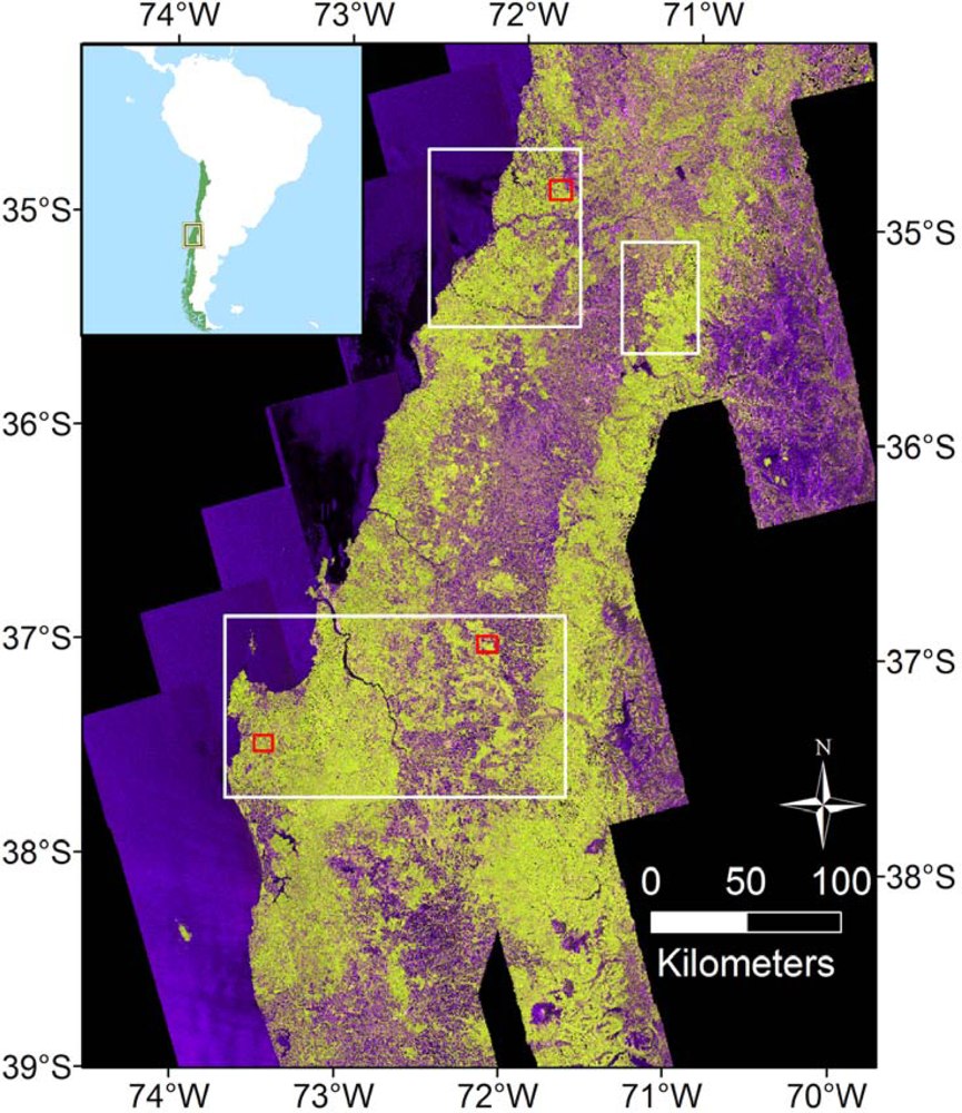
The study area in Central Chile extended over three Chilean administrative regions (Maule, Biobio, and Araucania) and covered parts of the coastal Cordillera and the Chilean Central Valley (Figure 1). The forests in the study area are dominated by even-aged plantations of Pinus radiata and to a lesser extent (<20% by area) Eucalyptus globulus[46]. Stand-level forest inventory data for 437 stands that were collected in the timeframe of the airborne lidar campaigns were provided by the ARAUCO timber company. The inventory data were delivered in the form of stand boundary maps with attached attribute tables. Stands in the inventory data were characterized by similar species, planting times and forest management practices. Within stands, field surveys were carried out in 0.25 ha sample plots. The plot density depended on the age and the species and varied between 0.25 and 1 plot per hectare. The plots are revisited every four years beginning eight years after planting and continuing until harvest (age 24–30). The inventory data provided information about the age, diameter at breast height (DBH), CH or stem density as well as derived parameters such as the basal area (BA) or the GSV. The DBH was measured for all stems in the plots using calipers. The canopy height (CH) referred to the dominant height (i.e., the height of the hundred tallest trees per hectare); the heights of five to seven trees per plot were actually measured in the field using clinometers. The growing stock volume (GSV) represented the volume of the merchantable portion of the tree stems [m3/ha], which does not include branches, stump and tip. The volume was estimated by means of species-specific taper functions. The relative stocking (RS) for each stand was determined by relating the observed basal area to that of the most productive stands in the same development stage (i.e., age). Among the 437 stands, 424 were pine stands and 13 were eucalyptus stands. The inventory data for the eucalyptus stands included GSV (61–442 m3/ha) but not CH. A summary of the pine stand characteristics is provided in Table 1.
2.2. Data
2.2.1. ALOS PALSAR
Under a NASA/JAXA data agreement we obtained from the Alaska Satellite Facility a multi-temporal ALOS PALSAR dataset over Central Chile. In total, 189 Fine Beam Dual-Polarization (FBD) and 181 Fine Beam Single-Polarization (FBS) images (Level 1.1 Single Look Complex) were downloaded from the ASF archives. The FBD data were acquired between June and December 2007 and the FBS data were acquired between January and June and November and December 2007. Ten FBD and 14 FBS images (from three different ALOS paths) covering the same area as the ALS data were used in this study. All images were acquired with a look angle of 35° (incidence angle range of 36.6° to 40.9°). Pre-processing of the SAR data was accomplished with software developed by GAMMA Remote Sensing ( http://www.gamma-rs.ch) and included absolute calibration [47], multi-looking (1 × 4 FBD, 2 × 4 FBS) and terrain-corrected geocoding with the aid of the 90 m SRTM-3 Digital Elevation Model (DEM) and the orbit data. The geocoded images were resampled to a regular map grid with 15 × 15 m2 pixel size (Projection: UTM Zone 18 South, Ellipsoid: WGS84). Radiometric correction for topographic effects included the compensation for topographic alterations of the pixel scattering area according to [48] and normalization with respect to the dependence of surface and volume backscatter on the local incidence angle [49]. Gamma-MAP filtering (7 × 7 pixels window size) was applied [50] to reduce speckle noise. A mosaic of FBD images for Central Chile is shown in Figure 1.
The interferometric coherence was computed for image pairs with temporal baselines of 46 or 92 days and all possible combinations of image modes, including FBD-FBD (HH-HH & HV-HV), FBS-FBS (HH-HH) as well as FBS-FBD (HH-HH) image pairs. The interferometric processing consisted of the oversampling (2×) of the FBD SLC in the case of FBS-FBD image pairs [51], co-registration of the Single Look Complex image pairs by means of cross-correlation of a large number of image chips, multi-looking, slope-adaptive range and azimuth common band filtering [52], adaptive coherence estimation with window sizes between 3 × 3 and 9 × 9 pixels and terrain-corrected geocoding and resampling to 15 × 15 m2 pixel size. In total, coherence images for 11 acquisition date combinations were produced (Table 2). The perpendicular baselines were between 40 and 900 m and thus significantly shorter than the critical baseline length (12.9 and 6.5 km for FBS and FBD, respectively) beyond which complete decorrelation due to nonoverlapping range spectra would occur.
2.2.2. Airborne Laser Scanner Data
The geospatial information company Digimapas Chile Aerofotogrametría Ltda. provided small-footprint airborne Lidar data for an area of ∼2.5 million ha in Central Chile (Figure 1). The data was acquired between November 2006 and 2008. The airborne platform that was used consisted of a laser scanning system (Riegl LMS-Q560), two digital cameras (Applanix DSS 322) and navigation equipment (Applanix POS AV 401). The Riegl LMS-Q560 Lidar has a nominal range resolution of 2 cm and delivers an absolute vertical and horizontal accuracy of better than 15 and 25 cm, respectively. During operation the height and intensity of multiple discrete laser returns for each laser pulse were recorded. The laser point density on the ground varied between 1 and 3 hits/m2 and the scan angles ranged up to 22.5°. Digimapas produced and delivered fully geocoded Digital Topographic (DTM) and Surface Models (DSM) with 1 × 1 m2 pixel spacing. The DTM was generated by filtering out vegetation returns and interpolating between ground (last) returns to obtain an estimate for the ground elevation. The DSM was computed from the first returns representing the top of the canopy in each 1 × 1 m2 grid cell. The vertical accuracy of the DTM was better than 0.75 m (pers. com. Markus Rombach, Digimapas Chile).
2.2.3. Landsat ETM+
From the Global Land Survey 2005, three Landsat 7 ETM+ images were obtained. Two images were acquired in 2005 (12/01/2005) and one in 2007 (01/30/2007) under cloud-free conditions over the study area in Central Chile. The images were downloaded from the Global Land Cover Facility ( http://www.landcover.org/). The L1T surface reflectance data were already calibrated and corrected for terrain as well as atmospheric effects [53]. Gaps in the data due to the SLC failure of the ETM+ instrument were filled for ∼98% with data from other acquisitions.
2.2.4. Weather Data
In order to investigate weather related effects on the SAR/InSAR observations, weather data were obtained for three weather stations from the US National Climatic Data Center (NCDC). Two weather stations were located in the Central Valley in Temuco (38.75°S, 72.633°W) and Curico (34.967°S, 71.233°W) and a third near the Pacific Coast in Concepcion (36.767°S, 73.067°W). The weather data included daily summaries of temperature, precipitation and wind conditions spanning all of 2007.
2.3. Data Preparation
2.3.1. Stand-Level Canopy Structure Indices
A Canopy Height Model (CHM) with 1 × 1 m2 pixel spacing was produced by subtracting the ALS DTM from the DSM. A suite of ALS canopy structure indices, characterizing different aspects of the forests canopy structure, were computed from the CHM for each stand in the inventory data. The indices that were computed comprised the percentiles of the height distribution of first returns in steps of 10% (referred to as relative heights RH10 to RH100), the coefficient of variation (CV), mean (ME), kurtosis (KT), skewness (SK) and several canopy density indices. Canopy density within each stand was estimated at four height intervals by dividing the height range between 2 m and RH90 into four equal-length bins [25,54] and estimating the proportion of first returns from heights above the respective height threshold, referred to as CD1 (returns > 2 m) to CD4. A Gaussian fit to the profile of first return heights was computed as an additional means of characterizing canopy vertical structure (i.e., with the number of Gaussians (NG) used to describe the profile). We followed the approach described in Hofton et al.[55] for large-footprint Lidar waveforms. For the Gaussian fit to the ALS canopy height profiles (see example in Figure 2), the single-bin peak at 0 m height (i.e., the forest floor) was not considered so that the Gaussian fit only reflected the vegetation profile. No more than three Gaussians were required to describe any of the canopy profiles.
From the ALOS PALSAR data, the average intensity and coherence were computed within each stand. From the Landsat ETM+ imagery, the average reflectance observed in bands 1 to 5 and 7 were computed.
2.3.2. Segmentation
In this study, we focused on the stand-level retrieval of GSV and CH because the stand scale is generally of greater interest to land managers. Image segmentation was therefore conducted on the ALS CHM using the multi-resolution segmentation algorithm implemented in the eCognition software package ( http://www.ecognition.com). Segmentation was used to delineate “stand-like” image object polygons across the study area. The eCognition multi-resolution segmentation algorithm considers within object variance, shape, compactness and smoothness parameters for the identification of homogeneous image objects and has shown good performance when used for the identification of homogeneous hectare-scale polygons from ALS CHMs [23]. For the segmentation, the CHM was aggregated by means of simple block averaging from 1 to 4 m pixels as a tradeoff between preserving spatial detail and reducing the amount of data to a level that could be handled by the software in an acceptable amount of time. The segmentation parameters (i.e., scale, compactness, smoothness) were chosen so that segments had sizes comparable to the polygons in the inventory dataset (on average 8 ha) and smoothly followed stand boundaries visible in the CHM. For the segments, the same set of ALS, ALOS PALSAR and Landsat canopy structure indices that were described in Section 2.3.1 were extracted. Segments for which RH90 was below 2 m and/or the canopy density (CD1) below 15% were labeled as non-forest and received no further consideration. By masking out all segments with low RH90 or CD1, we were able to ensure that all ALS canopy structure indices that were extracted from the segments and inventory polygons, respectively, varied within similar bounds. Very small segments < 0.5 ha (∼1% of all segments) were discarded from the dataset.
2.4. Modeling
For modeling the relationship between the suite of space- and airborne-remote sensing data and the in situ measurements of CH and GSV we used randomForest [43], a popular ensemble regression tree algorithm. In randomForest, a large number of regression trees are grown, each recursively partitioning the training data, considering at every node a random selection of predictors. The predictions from all regression trees are then averaged to obtain a single estimate. Each regression tree is grown using a random selection of samples. The rest of the samples, the so-called ‘out-of-bag’ cases (OOB), are estimated via the respective regression trees after training and the obtained OOB predictions for all trees are then averaged to obtain an unbiased estimate for the retrieval error. The randomForest package also provides tools for evaluating the importance of the different predictors. The appraisal of the predictor importance is accomplished by randomly permuting the values of a particular predictor (OOB cases) while keeping all other predictors unchanged and putting the data down the developed regression trees. The change of the retrieval error then allows inferring on the particular predictors’ ability to increase the node purity [56]. The performance of randomForest has been found comparable to other machine learning techniques and superior to single regression trees or multivariate regression models when used for predicting forest biophysical parameters from remotely sensed data [41,45,57]. Its robustness, computational efficiency and user friendliness have made randomForest one of the most applied modeling approaches for the mapping of forest resources at large spatial scales [13,14,17,41,44,45,57]. A Matlab port (available at http://code.google.com/p/randomforest-matlab/) to the original Fortran randomForest code of Breiman and Cutler was used in this study. In a two stage up-scaling approach, randomForest was used for the modeling of 1) the relationship between the ALS canopy structure indices and the in situ measurements of CH and GSV and 2) the relationship between the ALS-based estimates of GSV and CH and the PALSAR/Landsat datasets.
2.5. Layout and Spatial Scale of Fusion Experiments
2.5.1. Test Sites
The development of fusion-based models incorporating the ALS, PALSAR and Landsat data was first performed within three 100 km2 test sites. The test sites were selected so that (1) a wide range of stand growth stages were covered, (2) no management activities (e.g., thinning, logging, etc.) had occurred during the image acquisition timeframe and (3) a cluster of inventory polygons (i.e., stands) was located within each site. Two of the selected test sites were located in the Cordillera along the Pacific coast and one in the Chilean Central Valley (Figure 1). In total, 105 inventory stands were located within the area of the three test sites. These 105 stands were used for validation purposes only (i.e., they were not used for the development of models, relating the ALS canopy structure indices to CH and GSV). Information pertaining to the topography, forest characteristics and ALOS data availability at each test site is summarized in Table 2. At each of the test sites, ALS-derived estimates of CH and GSV for the segments in the ALS CHM were used as response variables in randomForest to develop new models, relating all available per-segment PALSAR intensities and coherences as well as Landsat reflectances to CH and GSV, respectively. The retrieval accuracy was assessed by (1) comparing the OOB estimates for CH and GSV to the per-segment ALS predictions of CH and GSV and (2) applying the developed models to the ALOS and Landsat data extracted for the inventory polygons that were located within the area of the test sites and comparing the obtained estimates for CH and GSV to the respective in situ measurements.
2.5.2. Extrapolation to Entire PALSAR Frames
The goal of a fusion of ALS and spaceborne data is eventually to extrapolate estimates of forest biophysical parameters from ALS samples (transects) to larger areas without ALS coverage. A key question in this respect is how the number of transects flown with ALS affects the retrieval performance. To this end, an experiment was carried out in which randomForest models were trained using a varying number of simulated ALS transects with constant distance and applying the models to predict the CH for entire PALSAR frames (∼70 × 70 km2). The extrapolation was tested for the southernmost area for which ALS data were available (i.e., the largest of the three ALS mosaics). The ALS CHM for this 189 × 90 km2 large area (see Figure 1) was divided into 600 m wide transects, each of which crossed the study area in East-West direction. The ALS canopy structure indices were used for estimating the CH for each of the segments in the ALS CHM. Segments for which less than 50% of their total area fell into a particular simulated transect were not considered as well as segments for which RH90 and CD1 were less than 2 m and/or 15%, respectively. 50% (150) of the simulated ALS transects (every other) were used for validation. The rest of the transects were considered for training randomForest models, relating the multi-temporal PALSAR FBD/FBS SAR/InSAR and Landsat observations to CH. Models were developed for two ALOS PALSAR paths. In each path, the parts of two consecutive PALSAR frames (i.e., both were acquired from the same orbit) that covered the ALS mosaic were mosaiced to form one image somewhat larger (∼90 × 70 km2) than a typical ALOS PALSAR frame (70 × 70 km2). One path covered test site 1 and the other test site 2 (i.e., the same set of intensity and coherence images that were listed in Table 2 was used). For each of the two paths, the corresponding subsets of the Landsat data mosaic were extracted.
3 Results and Discussion
3.1. Stand-Level Retrieval of CH and GSV with ALS
3.1.1. Retrieval Accuracy
For the stand-level retrieval of CH and GSV by means of the ALS data, randomForest was applied using the default values for the number of regression trees that are grown (500), the number of randomly selected predictors that are considered at each node (the square root of the total number of predictors) as well as the percentage of bootstrap samples (OOB) that are used for each added regression tree to obtain an estimate of the retrieval error (33%). Figure 3 illustrates the stand-level OOB estimates for GSV and CH when using all stand-level ALS canopy structure indices as predictors and the in situ measurements of CH and GSV obtained from 319 pine stands as response variables. The retrieval accuracy is given with the coefficient of determination (R2), the root mean square error (RMSE), the relative RMSE (RMSEr) and the bias. The RMSEr represented the RMSE divided by the average GSV and CH in the in situ dataset and the bias was calculated from the difference between the average GSV and CH in the in situ dataset and the ALS predictions, respectively.
In the case of the GSV retrieval, the R2 was 0.81, the RMSE was 62 m3/ha and the relative RMSE was 22% when comparing the randomForest OOB predictions to the inventory data. In the case of CH, the R2 was 0.93, the RMSE was 1.7 m and the RMSEr was 7.1%. The bias was negligible in both cases. When using independent sets of training (67%) and testing samples (33%), the retrieval accuracies did not differ significantly (in the range of 1%) from the OOB results. The number of eucalyptus stands in the inventory dataset (13) was too low for developing a species-specific model. When applying the model developed for pine to predict the GSV of the eucalyptus stands in the inventory dataset, the retrieval accuracy was high (RMSE = 36.5 m3/ha, RMSEr = 18%, R2 = 0.95, bias = −1.9 m3/ha).
3.1.2. Information Content of the ALS Canopy Structure Indices
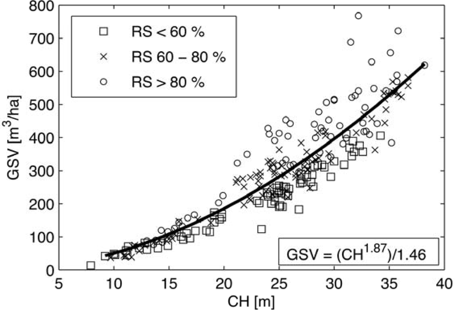
The randomForest predictor importance ranking (Figure 4) suggested that the higher range of relative heights (except RH100) were most important for the retrieval of the CH as well as GSV. The most important predictor in both cases was RH90. Overall, the randomForest predictor importance ranking for the retrieval of CH and GSV revealed only minor differences. Noticeable differences were only observed in the lower range of relative heights (RH30), which appeared to be somewhat more important for the retrieval of GSV. The most important predictors according to randomForest were highly correlated. The correlation of the relative heights RH50 to RH90, for instance, was always >0.98, suggesting substantial redundancy between the predictors. Also the response variables CH and GSV revealed a high correlation of 0.84 (Figure 5). The correlation further increased when only considering stands with similar RS. For stands with a RS > 80%, for instance, the correlation of CH and GSV increased to 0.91.
In order to appraise the information content of the different ALS canopy structure indices with respect to the forests structural properties in the vertical and horizontal forest growth dimensions, accounting for the correlation between the predictor as well as the response variables, we also conducted a Canonical Correlation Analysis (CCA). In a CCA, which allows investigating interrelationships between two sets of variables (e.g., a set of predictor and response variables), weights for each variable are computed that maximize the correlation between weighted linear combinations (the canonical variables) of the variables in each of the two datasets [58,59]. Subsequent canonical variables maximize the correlation between the two datasets while minimizing the correlation with respect to prior canonical variables. For the CCA, we first considered the full set of ALS canopy structure indices in the first (predictor) and the in situ estimates of CH and GSV in the second (response) dataset. The CCA generated two canonical variable pairs for which we calculated the Pearson correlations (r) with the respective variables in the predictor and response datasets (the so-called canonical factor loadings). The canonical correlations between the two canonical variable pairs were 0.97 and 0.49, respectively. Both canonical correlations were statistically significant (F-test, P < 0.0001). The first pair of canonical variables, which accounted for most (87%) of the variance in the ALS dataset, was highly correlated to CH (r > 0.99) and RH90 (r = 0.99), respectively. The second canonical variable pair was most correlated to GSV (r = −0.46) and the KT (r = 0.65), RH10 (r = −0.49) and RH20 (r = −0.47) indices, respectively. The CCA hence pointed out the precedence of height related information in the ALS first/last return data. The second canonical variable pair suggested though that some of the ALS canopy structure indices (i.e., the KT or the lower range of relative heights) added information about forest structural differences in the horizontal forest growth dimension. We also conducted the CCA with other inventory parameters in the response dataset (e.g., BA, DBH, RS) and observed that, while the first canonical variable was always highly correlated to CH (r > 0.99), the second canonical variable was most correlated to RS (r ∼ 0.9), which describes basal area differences between stands with similar CH but different GSV (Figure 5).
The CCA as well as the overall minor differences in the randomForest predictor importance ranking (Figure 4) for the retrieval of CH and GSV suggested that the retrieval of GSV, an attribute that necessarily integrates horizontal and vertical forest structure, largely reflected the allometric relationship between CH and GSV. This suggestion was confirmed when converting the randomForest OOB CH estimates to GSV using the allometric relationship shown in Figure 5; the allometric equation was derived by means of regression. In this case, the GSV retrieval accuracy was only slightly lower than that achieved with the randomForest model trained on in situ GSV directly (RMSEr = 25%, R2 = 0.76, bias = 1.1 m3/ha). The high accuracy of the GSV retrieval in the case of the Central Chilean study area may therefore be attributed to the fact that in plantations the GSV is highly correlated to CH.
The limited capability of the ALS first/last return data to explain the GSV variability due to forest structural differences in the horizontal forest growth dimension for stands with similar CH entails that, in order to produce GSV estimates without systematic bias when extrapolating from field data to ALS transects and eventually to the area covered by the spaceborne imagery, a rather large in situ dataset is required to cover not only the full range of GSV but also the regional distribution of RS, which influences the allometric relationship between CH and GSV (cf. [60]). For example, when models for the prediction of GSV are developed for stands with high RS (> 80%) and then used to estimate the GSV for stands with lower RS (<60%), the estimates are strongly biased (RMSE = 85.2 m3/ha, RMSEr = 36%, R2 = 0.79, bias = 60 m3/ha) whereas the CH retrieval remains unbiased (RMSE= 2.1 m, RMSEr = 9.0%, R2 = 0.89, bias = 0.02 m). More detailed information about the forests horizontal structure may be inferred from ALS data when not only considering the first/last returns but also the returns from within the canopies. Also a stratified modeling approach might help to reduce systematic biases in the GSV estimates. In Gobakken et al.[61], for instance, separate models were developed for different forest productivity classes that were classified by means of existing land use maps, elevation models and Landsat data for a county in Norway.
3.2. CH and GSV Retrieval through Synergy of ALS, PALSAR & Landsat
3.2.1. Retrieval with All Spaceborne L-Band SAR/InSAR and Optical Images
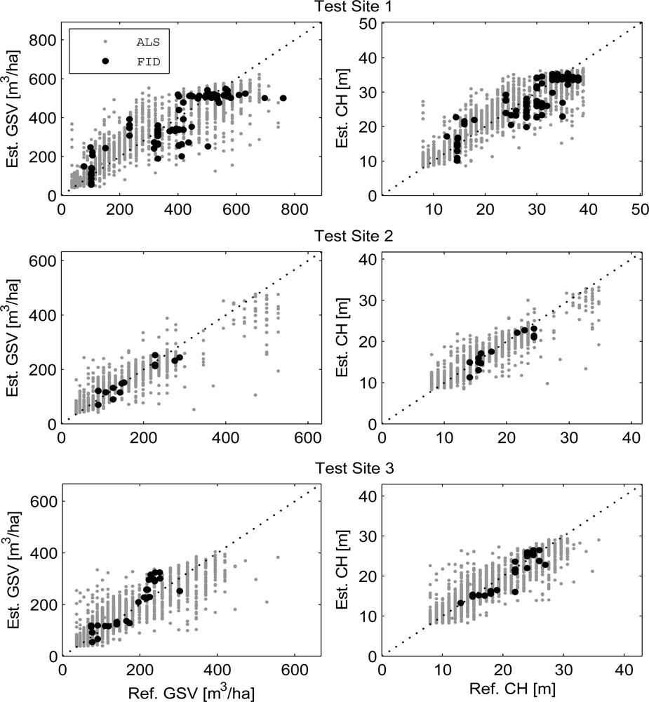
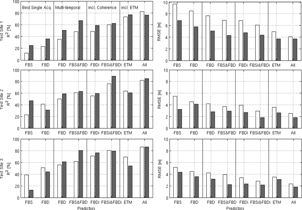
Table 3 summarizes the accuracies of the randomForest CH and GSV retrieval at the three test sites when using all available spaceborne predictor layers (i.e., up to 18 layers incl. multi-temporal PALSAR HH&HV intensities, repeat-pass coherences and Landsat ETM+ reflectances) and the ALS-based per-segment estimates for CH and GSV as response variables. Figure 6 illustrates the agreement of the obtained CH and GSV estimates for the segments and inventory polygons with the ALS-based estimates and in situ measurements, respectively.
When comparing the OOB estimates of CH and GSV with the per-segment estimates from ALS, similar accuracies in terms of the R2 and RMSEr were obtained at the three test sites. In the case of GSV, the R2 was ∼0.8 and the RMSEr was below 30% for all three test sites. In the case of CH, the R2 was ∼0.82–0.86 and the RMSEr was in the range of 15 to 17%. The RMSEs at test sites 2 and 3 were about 43 m3/ha (GSV) and 2.5 m (CH), respectively. At test site 1, the RMSEs were higher but since the average GSV and CH values were also higher, the RMSEr was comparable to that obtained at the other two sites. The bias was always close to zero. The result of the independent validation using 105 inventory stands was consistent with those obtained when comparing the PALSAR/Landsat OOB estimates for CH and GSV to the respective ALS derived estimates. In the case of GSV, the R2 was between 0.72 and 0.87 and the RMSEr between 15 and 25%. In the case of CH, the R2 was between 0.76 and 0.86 and the RMSEr between 8 and 13%. The GSV and CH estimates for the inventory polygons generally presented a somewhat larger bias of up to 20 m3/ha and 1 m, respectively.
3.2.2. Benefit of the Fusion of Multi-Temporal L-Band SAR/InSAR and Landsat Data
In order to evaluate the benefit of integrating multi-temporal PALSAR FBD and FBS intensity images, repeat-pass coherence and Landsat, we repeated the CH retrieval using different combinations of the spaceborne datasets; note that we focused on the CH retrieval because the GSV estimates simply represented the allometric relationship between CH and GSV (see Section 3.1.2). Eight different combinations of predictors were considered: (1) the best FBS intensity image (1×HH), (2) the best FBD intensity image (1×HH, 1×HV), (3) all FBD intensity images (2×HH, 2×HV), (4) all FBS/FBD intensity images (4–5×HH, 2×HV), (5) all FBD intensity (2×HH, 2×HV) and coherence images (1×HH, 1×HV), (6) all FBS/FBD intensity (4–5×HH, 2×HV) and coherence images (2–4×HH, 1×HV), (7) Landsat only, (8) Landsat and all FBS/FBD intensity (4–5×HH, 2×HV) and coherence images (2–4×HH, 1×HV).
The retrieval accuracies that were achieved when using intensities from only one FBS or FBD acquisition were low with less than 50% of CH variance being explained and RMS errors in the range of 4 to 6 m at test sites 2 and 3 and 8 to 10 m at test site 1 (i.e., the test site with the highest average and maximum CH) when comparing the randomForest OOB against the ALS estimates (Figure 7). As was to be expected, the retrieval with the FBD images performed somewhat better than the retrieval with FBS since the FBD images included the HV intensity. The integration of multi-temporal intensity observations allowed substantial improvements of the retrieval performance. When combining all available FBD intensities, the R2 and RMSE improved for about 5 to 12% and 0.25 to 0.8 m, respectively. The R2 and RMSE improved further when adding the stack of FBS intensity images for 6.5 to 12% (R2) and 0.3 to 0.7 m (RMSE). The integration of the coherence images resulted as well in higher retrieval accuracies. When using all available FBS/FBD intensities and coherences, the R2 and RMSE were in the range of 0.75 to 0.8 and 3 m at test sites 2 and 3 and 0.60 and 6 m at test site 1, respectively. Finally, the R2 and RMSE improved significantly for 6 to 22% and 0.4 to 2 m, respectively, when adding the Landsat data to the stack of multi-temporal intensities and coherences. When testing the retrieval with only the Landsat data, the retrieval accuracy was roughly comparable to that achieved with the multi-temporal PALSAR intensities at test sites 2 and 3. At test site 1 (the test site with the highest average and maximum CH), the Landsat image even outperformed the PALSAR imagery with only minor improvements being achieved when combining the PALSAR and Landsat imagery.
The improvement of the retrieval accuracy with the successive integration of multi-temporal intensities, coherences and Landsat was generally confirmed when comparing the randomForest predictions for the inventory polygons to the corresponding in situ measurements, albeit a number of exceptions were noticed. At test site 1, for instance, the R2 decreased for about 5% when adding the coherences to the stack of multi-temporal FBD/FBS intensities and at test site 2, the retrieval with the best FBS intensity image performed better than the retrieval with the best FBD image. The reason for these contradictory results was not clear; they may be sporadic effects due to the much smaller sample size in the inventory datasets.
3.2.3. Contribution of SAR, InSAR and Optical Datasets
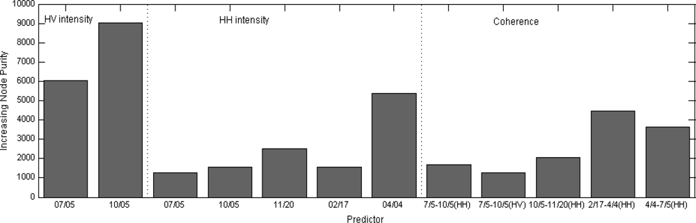
According to the randomForest predictor importance ranking, the HV intensity images were always amongst the most important predictors for the retrieval of CH and GSV at all test sites, albeit with some differences between the acquisition dates. Figure 8 illustrates the predictor ranking for the CH retrieval with all PALSAR intensities and coherences at test site 2. With one exception, the importance of the HH intensity images was low. In relative terms, the importance of the coherence images tended to be in a “low” to “medium” range compared to the best HV intensity images.
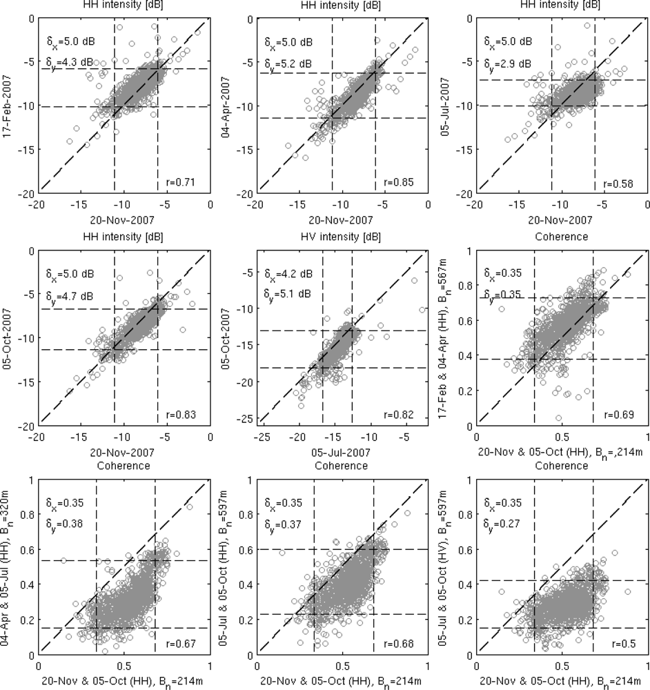
The randomForest importance ranking not only reflected the different data types (i.e., intensity/coherence, HH/HV polarization) but also the changing weather (e.g., rain) and environmental (e.g., soil moisture) conditions. At all test sites, the multi-temporal consistency of the L-band intensity images was high (Pearson correlations mostly above 0.8), confirming what has been reported for other forest sites [31,62,63]. Figure 9 illustrates the multi-temporal consistency of the intensity and coherence images covering test site 2 and the dynamic ranges that were defined with the 5th and 95th percentiles. When comparing intensity images that were acquired under dry and rainy conditions, respectively, those that were acquired under rainy conditions revealed clear deviations from the 1:1 line, lower dynamic ranges and, in the case of HH polarization, lower multi-temporal correlations between the per-segment intensities in the range of 0.6 to 0.7. Consequently, at test site 2 the HV intensity image that was acquired under rainy conditions on 5 July contributed less to the retrieval than the HV image from 5 October (Figure 8). In the case of the HH intensity images, those that were acquired under rainy conditions (5 July, 17 February) always ranked low in the randomForest predictor importance ranking. However, the effect of rain did not entirely explain the differences in the importance ranking. The HH intensity images from 5 October and 20 November, for instance, were less important for the retrieval than the intensity image from 4 April although all three images were acquired during dry periods and had similar dynamic ranges.
The multi-temporal consistency of the coherence images was lower than that of the intensity images with correlations in the range of 0.5 to 0.7 (Figure 9). At all three test sites, the lowest correlations of ∼0.5 were observed when one of the two images that were compared was a HV coherence image. The dynamic range of the HH coherence images was consistently in the range of 0.3 to 0.35; in the case of HV, the dynamic range was always lower than 0.3. Compared to the intensity observations, the effect of rain on the coherence was not as evident. Rain events have been reported to cause substantial decorrelation that strongly diminishes forest related information in repeat-pass coherence images because of the pronounced associated changes in the dielectric properties of the soils and canopies [36,37]. At test site 2, however, the coherence for the HH image pair from 17 February & 4 April revealed the overall highest coherence amongst the available coherence images although all three weather stations reported continuous rainfall of 2 to 4 cm in the two days prior to the sensor overpass on 17 February. The two HH coherence images that were computed from the 5 July acquisition (both with 92 day temporal baseline), for which the weather stations in Concepcion and Temuco reported about 1.5 cm of rainfall in the two days prior to the acquisition, were instead characterized by an overall lower coherence (but similar dynamic range) than the other two HH coherence images at test site 2. Also the wind speeds and the perpendicular baselines may have influenced the coherence since strong winds and long baselines are associated with stronger temporal and volume decorrelation over forest [64]. The baseline lengths and the wind conditions recorded at the weather stations in Concepcion, Temuco and Curico did, however, not provide any immediate explanation for the different coherence levels that were observed. In order to differentiate the combined effects of temporal and volume decorrelation and to evaluate their respective effects on the sensitivity of the coherence to forest biophysical quantities, a physically-based modeling approach would be required, which was beyond the scope of this study.
According to the randomForest predictor ranking (Figure 8), the HH coherence images from 17 February and 4 April and 4 April and 5 July (i.e., one 46- and one 92-day repeat-pass image) contributed most to the CH retrieval at test site 2. When looking at the correlations between coherence and the ALS derived per-segment estimates of CH (between −0.2 and −0.6 at all test sites), the coherence images that were most important for the retrieval were not necessarily those with the highest correlation to CH. In the case of the coherence image from 17 February and 4 April, for instance, the correlation was only −0.23. A comparison of the CH estimates obtained when using (1) only the multi-temporal intensities and (2) the multi-temporal intensities and coherences at the three test sites revealed that the coherence images primarily influenced the retrieval in the higher CH ranges (Figure 10). This observation suggested a higher sensitivity of coherence to CH in dense and a lower sensitivity in sparse forests compared to intensity.
In Section 3.2.2, we reported significant improvements of the retrieval performance when adding the Landsat images to the stack of ALOS PALSAR imagery. As for coherence, we analyzed if the integration of the Landsat imagery improved the retrieval in specific ranges of CH. There were, however, no apparent trends noticeable (i.e., the Landsat integration improved the estimates throughout the entire range of CH). The results pointed out that, wherever the cloud conditions allow, the fusion of SAR and multispectral optical data should be considered since the best retrieval results were generally achieved when adding the Landsat images to the stack of PALSAR intensity and coherence images. In accordance with what was reported by others [14,45,57], the randomForest predictor importance ranking indicated that the short wave infrared (SWIR) reflectances (Landsat ETM+ bands 5 and 7) were crucial for the retrieval. In Baccini et al.[14], the increased sensitivity of the SWIR bands to forest biophysical parameters such as aboveground biomass was explained with the limited diffuse radiation and the hence increased influence of shadow effects, which depend on the canopy density and structure.
3.3. Extrapolation to ALOS PALSAR Frames
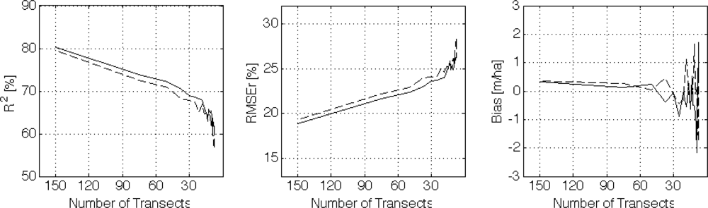
Figure 11 shows for the CH retrieval at the scale of an entire PALSAR frame how the retrieval performance changed when systematically reducing the number of ALS transects. When using 50% (150) of the simulated ALS transects (i.e., all transects that were not part of the validation dataset) in the area covered by the respective PALSAR paths for training randomForest and applying the developed models to predict the CH with the same set of PALSAR/Landsat imagery for the segments in the transects that were kept aside for validation, the comparison of the obtained estimates and the corresponding ALS based estimates resulted in a R2 and RMSEr of ∼0.8 and 18%, respectively. The retrieval accuracy was thus comparable to that obtained at the small test sites (cf. Table 3). Figure 11 shows that the retrieval accuracy decreased continuously when systematically reducing the number of ALS transects (i.e., retaining equal distances between the transects) used for training randomForest. When using 10% (30) of the transects covered by the particular ALOS paths for model training, the R2 and RMSEr were in the range of 0.7 and 24%, respectively. Concomitantly, the bias of the PALSAR/Landsat predictions remained low as long as more than ∼10% of the simulated ALS transects were used for model training (Figure 11, right plot).
The results of the extrapolation experiment indicated rather high sampling requirements to achieve retrieval accuracies that were achieved at smaller test sites also at larger scale (i.e., 50% of the study area). When having ALS data for about 10% of the area covered by an ALOS PALSAR frame, the loss in retrieval performance remains moderate though (∼10% lower R2). A 10% coverage with ALS might be practical when flying the ALS in higher altitudes, which in turn, however, can be expected to affect the retrieval performance because higher flight altitudes result in lower laser point densities on the ground [65]. On the other hand, ALS sampling in form of random or stratified random flight patterns [8] might allow reducing the required ALS sampling density.
4. Conclusions
We have demonstrated for the showcase scenario of forest plantations in Central Chile the feasibility of a stand-level retrieval of canopy height and growing stock volume through the two-stage fusion of field, airborne laser scanner, multi-temporal ALOS PALSAR L-band intensity, repeat-pass coherence and Landsat ETM+ multispectral data. At three 100 km2 test sites, the retrieval of canopy height and growing stock volume with the PALSAR and Landsat imagery reached promising accuracies with R2s in the range of 0.7 to 0.85 when training randomForest ensemble regression tree models with laser scanner based stand-level estimates of canopy height and growing stock volume as surrogate reference data. We were able to show that the combined use of multi-temporal PALSAR intensity, interferometric repeat-pass coherence and Landsat reflectances as predictors in randomForest allowed consistently higher accuracies than the retrieval with any of the datasets alone. The results of this study therefore re-emphasized the importance of fusion algorithms for making optimal use of the forest structural information contained in the wealth of data acquired by spaceborne radar and optical missions such as ALOS PALSAR and Landsat.
In this study, the retrieval of canopy height and growing stock volume by means of the fusion of lidar, radar and optical remote sensing was tested only for plantation forests. It is therefore advised to test the retrieval approach at other forest sites to evaluate its performance in structurally more diverse forest ecosystems. Another issue that will have to be addressed is the lidar sample survey design. Our initial investigations indicated dense laser scanner sampling requirements (at least 10% of the study area) when extrapolating from a number of simulated laser scanner transects with a systematic survey design (i.e., constant distance between transects) to larger areas using the PALSAR and Landsat imagery. The sampling requirements (and the associated costs of the airborne lidar campaign) might be reduced significantly when optimizing the sample survey design (e.g., with stratified random flight lines [8]).
With an increasing number of commercial vendors offering the acquisition of airborne laser scanner data, the novel fusion approach presented above could be a viable option for the regional scale mapping of canopy height and growing stock volume in many forest regions. However, the ALOS PALSAR mission ended in 2011 so that currently no L-band radar data are acquired from space. With the planned ALOS-2 and DESDynI-R L-band radar missions as well as the Landsat Data Continuity Mission, a similar approach for the fusion of lidar, radar and optical data will also be possible in the future. The L-band ALOS-2 and DESDynI-R missions will likely provide for a number of improvements over ALOS PALSAR, such as a more consistent multi-annual coverage and shorter repeat intervals for improved interferometric applications (e.g., of coherence), so that improvements with respect to the retrieval performance can be expected.
Acknowledgments
The work presented in this paper was supported by the NASA funded project “Ecosystem Structure Measurements from DESDynI: Studies of technological options and data fusion using IceSAT/GLAS, Airborne Lidar and ALOS/PALSAR data sets over Central Chile” (NASA Grant #NNX08AL17G). Sergio Gonzales (Forestal Arauco) is acknowledged for the provision of the inventory data.
References
- Lefsky, M.; Harding, D.; Cohen, W.B.; Parker, G.; Shugart, H. Surface lidar remote sensing of Basal area and biomass in deciduous forests of Eastern Maryland, USA. Remote Sens. Environ 1999, 67, 83–98. [Google Scholar]
- Lefsky, M.; Cohen, W.B.; Parker, G.; Harding, D. Lidar remote sensing for ecosystem studies. BioScience 2002, 52, 19–30. [Google Scholar]
- Means, J.E.; Acker, S.A.; Harding, D.J.; Blair, J.B.; Lefsky, M.A.; Cohen, W.B.; Harmon, M.E.; McKee, W.A. Use of large-footprint scanning airborne lidar to estimate forest stand characteristics in the Western Cascades of Oregon. Remote Sens. Environ 1999, 67, 298–308. [Google Scholar]
- Drake, J.B.; Dubayah, R.; Knox, R.; Clark, D.B.; Blair, J. Sensitivity of large-footprint lidar to canopy structure and biomass in a neotropical rainforest. Remote Sens. Environ 2002, 81, 378–392. [Google Scholar]
- Anderson, J.; Martin, M.; Smith, M.; Dubayah, R.; Hofton, M.; Hyde, P.; Peterson, B.; Blair, J.; Knox, R. The use of waveform lidar to measure northern temperate mixed conifer and deciduous forest structure in New Hampshire. Remote Sens. Environ 2006, 105, 248–261. [Google Scholar]
- Bergen, K.; Goetz, S.; Dubayah, R.; Henebry, G.M.; Hunsaker, C.T.; Imhoff, M.L.; Nelson, R.; Parker, G.G.; Radeloff, V.C. Remote sensing of vegetation 3-D structure for biodiversity and habitat: Review and implications for lidar and radar spaceborne missions. J. Geophys. Res. 2009, 114, G00E06,. 1–13. [Google Scholar]
- Lefsky, M.; Ramond, T.; Weimer, C.S. Alternate spatial sampling approaches for ecosystem structure inventory using spaceborne lidar. Remote Sens. Environ 2011, 115, 1361–1368. [Google Scholar]
- Wulder, M.A.; White, J.; Nelson, R.; Næsset, E.; Ørka, H.O.; Coops, N.C.; Hilker, T.; Bater, C.W.; Gobakken, T. Lidar sampling for large-area forest characterization: A review. Remote Sens. Environ 2012, 121, 196–209. [Google Scholar]
- Boudreau, J.; Nelson, R.; Margolis, H.; Beaudoin, A.; Guindon, L.; Kimes, D. Regional aboveground forest biomass using airborne and spaceborne LiDAR in Québec. Remote Sens. Environ 2008, 112, 3876–3890. [Google Scholar]
- Nelson, R.; Ranson, K.J.; Sun, G.; Kimes, D.; Kharuk, V.; Montesano, P.M. Estimating Siberian timber volume using MODIS and ICESat/GLAS. Remote Sens. Environ 2009, 113, 691–701. [Google Scholar]
- Lefsky, M.A. A global forest canopy height map from the Moderate Resolution Imaging Spectroradiometer and the Geoscience Laser Altimeter System. Geophys. Res. Lett 2010, 37, 1–5. [Google Scholar]
- Saatchi, S.S.; Harris, N.; Brown, S.; Lefsky, M.; Mitchard, E.T.; Salas, W.; Zutta, B.R.; Buerman, W.; Lewsi, S.L.; Hagen, S.; Petrova, S.; White, L.; Silman, M.; Morel, A. Benchmark map of forest carbon stocks in tropical regions across three continents. Proc. Natl. Amer. Sci 2011, 108, 9899–9904. [Google Scholar]
- Simard, M.; Pinto, N.; Fisher, J.B.; Baccini, A. Mapping forest canopy height globally with spaceborne lidar. J. Geophys. Res 2011, 116, 1–12. [Google Scholar]
- Baccini, A.; Goetz, S.; Walker, W.S.; Laporte, N.; Sun, M.; Sulla-Menashe, D.; Hackler, J.; Beck, P.S.A.; Dubayah, R.; Friedl, M.A.; Samanta, S.; Houghton, R.A. Estimated carbon dioxide emissions from tropical deforestation improved by carbon-density maps. Nature Clim. Change 2012, 2, 1–4. [Google Scholar]
- Wulder, M.A.; Seemann, D. Forest inventory height update through the integration of LIDAR data with segmented Landsat imagery. Can. J. Remote Sens 2003, 29, 536–543. [Google Scholar]
- Hudak, A.; Lefsky, M.; Cohen, W.B.; Berterretche, M. Integration of lidar and Landsat ETM+ data for estimating and mapping forest canopy height. Remote Sens. Environ 2002, 82, 397–416. [Google Scholar]
- Kellndorfer, J.; Walker, W.; LaPoint, E.; Kirsch, K.; Bishop, J.; Fiske, G. Statistical fusion of lidar, InSAR, and optical remote sensing data for forest stand height characterization: A regional-scale method based on LVIS, SRTM, Landsat ETM+, and ancillary data sets. J. Geophys. Res. 2010, 115, G00E08,. 1–10. [Google Scholar]
- Englhart, S.; Keuck, V.; Siegert, F. Aboveground biomass retrieval in tropical forests—The potential of combined X- and L-band SAR data use. Remote Sens. Environ 2011, 115, 1260–1271. [Google Scholar]
- Sun, G.; Ranson, K.J.; Guo, Z.; Zhang, Z.; Montesano, P.; Kimes, D. Forest biomass mapping from lidar and radar synergies. Remote Sens. Environ 2011, 115, 2906–2916. [Google Scholar]
- He, Q.S.; Cao, C.H.; Chen, E.; Sun, G.Q.; Ling, F.L.; Pang, Y.; Zhang, H.; Ni, W.J.; Xu, M.; Li, Z.; Li, X.W. Forest stand biomass estimation using ALOS PALSAR data based on LiDAR-derived prior knowledge in the Qilian Mountain, western China. Int. J. Remote Sens 2012, 33, 710–729. [Google Scholar]
- Magnussen, S.; Boudewyn, P. Derivations of stand heights from airborne laser scanner data with canopy-based quantile estimators. Can. J. For. Res 1998, 28, 1016–1031. [Google Scholar]
- Means, J.E.; Acker, S.A.; Fltt, B.J.; Renslow, M.; Hendrix, C.J. Predicting forest stand characteristics with Airborne Scanning Lidar. Photogramm. Eng. Remote Sensing 2000, 66, 1367–1371. [Google Scholar]
- Van Aardt, J.A.N.; Wynne, R.H.; Oderwald, R.G. Lidar-distributional parameters on a per-segment basis. For. Sci 2006, 52, 636–649. [Google Scholar]
- Næsset, E. Predicting forest stand characteristics with airborne scanning laser using a practical two-stage procedure and field data. Remote Sens. Environ 2002, 80, 88–99. [Google Scholar]
- Næsset, E.; Gobakken, T. Estimation of above- and below-ground biomass across regions of the boreal forest zone using airborne laser. Remote Sens. Environ 2008, 112, 3079–3090. [Google Scholar]
- Nord-Larsen, T.; Schumacher, J. Estimation of forest resources from a country wide laser scanning survey and national forest inventory data. Remote Sens. Environ 2012, 119, 148–157. [Google Scholar]
- Lindberg, E.; Hollaus, M. Comparison of methods for estimation of stem volume, stem number and basal area from airborne laser scanning data in a hemi-boreal forest. Remote Sens 2012, 4, 1004–1023. [Google Scholar]
- Asner, G.P.; Powell, G.; Mascaro, J.; Knapp, D.E.; Clark, J.K.; Jacobson, J.; Kennedy-Bowdoin, T.; Balaji, A.; Paez-Acosta, G.; Victoria, E.; Secada, L.; Valqui, M.; Hughes, R.F. High-resolution forest carbon stocks and emissions in the Amazon. PNAS 2010, 107, 16738–16742. [Google Scholar]
- Rosenqvist, A.; Shimada, M.; Ito, N.; Watanabe, M. ALOS PALSAR: A pathfinder mission for global-scale monitoring of the environment. IEEE Trans. Geosci. Remote Sens 2007, 45, 3307–3316. [Google Scholar]
- Kurvonen, L.; Pulliainen, J.T.; Hallikainen, M.T. Retrieval of biomass in boreal forests from multitemporal ERS-1 and JERS-1 SAR images. IEEE Trans. Geosci. Remote Sens 1999, 37, 198–205. [Google Scholar]
- Askne, J.I.H.; Santoro, M.; Smith, G.; Fransson, J.E.S. Multitemporal repeat-pass SAR interferometry of boreal forests. IEEE Trans. Geosci. Remote Sens 2003, 41, 1540–1550. [Google Scholar]
- Rauste, Y. Multi-temporal JERS SAR data in boreal forest biomass mapping. Remote Sens. Environ 2005, 97, 263–275. [Google Scholar]
- Santoro, M.; Eriksson, L.E.B.; Askne, J.I.H.; Schmullius, C.C. Assessment of stand-wise stem volume retrieval in boreal forest from JERS-1 L-band SAR backscatter. Int. J. Remote Sens 2006, 27, 3425–3454. [Google Scholar]
- Santoro, M.; Beer, C.; Cartus, O.; Schmullius, C.C.; Shvidenko, A.; McCallum, I.; Wegmüller, U.; Wiesmann, A. Retrieval of growing stock volume in boreal forest using hyper-temporal series of Envisat ASAR ScanSAR backscatter measurements. Remote Sens. Environ 2011, 115, 490–507. [Google Scholar]
- Cartus, O.; Santoro, M.; Kellndorfer, J. Mapping of forest aboveground biomass in the northeastern United States with ALOS PALSAR dual-polarization L-Band. Remote Sens. Environ 2012, 124, 466–478. [Google Scholar]
- Eriksson, L.E.B.; Santoro, M.; Wiesmann, A.; Schmullius, C.C. Multitemporal JERS repeat-pass coherence for growing-stock volume estimation of Siberian forest. IEEE Trans. Geosci. Remote Sens 2003, 41, 1561–1570. [Google Scholar]
- Simard, M.; Hensley, S.; Lavalle, M.; Dubayah, R.; Pinto, N.; Hofton, M. An empirical assessment of temporal decorrelation using the uninhabited aerial vehicle synthetic aperture radar over forested landscapes. Remote Sens 2012, 4, 975–986. [Google Scholar]
- Tsui, W.O.; Coops, N.C.; Wulder, M.A.; Marshall, P.L.; McCardle, A. Using multi-frequency radar and discrete-return LiDAR measurements to estimate above-ground biomass and biomass components in a coastal temperate forest. ISPRS J. Photogramm 2012, 69, 121–133. [Google Scholar]
- Rignot, E.; Salas, W.; Skole, D. Mapping deforestation and secondary growth in Rondonia, Brazil, using imaging radar and thematic mapper data. Remote Sens. Environ 1997, 59, 167–179. [Google Scholar]
- Moghaddam, M.; Dungan, J.; Acker, S. Forest variable estimation from fusion of SAR and multispectral optical data. IEEE Trans. Geosci. Remote Sens 2002, 40, 2176–2187. [Google Scholar]
- Walker, W.; Kellndorfer, J.M.; Lapoint, E.; Hoppus, M.; Westfall, J. An empirical InSAR-optical fusion approach to mapping vegetation canopy height. Remote Sens. Environ 2007, 109, 482–499. [Google Scholar]
- Chen, W.; Blain, D.; Li, J.; Keohler, K.; Fraser, R.; Zhang, Y.; Leblanc, S.; Olthof, I.; Wang, J.; McGovern, M. Remote Biomass measurements and relationships with Landsat-7/ETM+ and JERS-1/SAR data over Canada’ s western sub-arctic and low arctic. Int. J. Remote Sens 2009, 30, 2355–2376. [Google Scholar]
- Breiman, L. Random forests. Mach. Learn 2001, 45, 5–23. [Google Scholar]
- Houghton, R.; Butman, D.; Bunn, A.G.; Krankina, O.N.; Schlesinger, P.; Stone, T.A. Mapping Russian forest biomass with data from satellites and forest inventories. Environ. Res. Lett 2007, 2, 45032. [Google Scholar]
- Avitabile, V.; Baccini, A.; Friedl, M.A.; Schmullius, C.C. Capabilities and limitations of Landsat and land cover data for aboveground woody biomass estimation of Uganda. Remote Sens. Environ 2012, 117, 366–380. [Google Scholar]
- Toro, J.; Gessel, S. Radiata pine plantations in Chile. New Forests 1999, 18, 33–44. [Google Scholar]
- Shimada, M.; Isoguchi, O.; Tadono, T.; Isono, K. PALSAR radiometric and geometric calibration. IEEE Trans. Geosci. Remote Sens 2009, 47, 3915–3932. [Google Scholar]
- Small, D. Flattening Gamma: Radiometric terrain correction for SAR imagery. IEEE Trans. Geosc. Remote Sens 2011, 49, 3081–3093. [Google Scholar]
- Castel, T.; Beaudoin, A.; Stach, N.; Stussi, N.; Le Toan, T.; Durand, P. Sensitivity of space-borne SAR data to forest parameters over sloping terrain. Theory and experiment. Int. J. Remote Sens 2001, 22, 2351–2376. [Google Scholar]
- Lopes, A.; Nezry, E.; Touzi, R.; Laur, H. Structure detection and statistical adaptive speckle filtering in SAR images. Int. J. Remote Sens 1993, 14, 1735–1758. [Google Scholar]
- Werner, C.; Wegmüller, U.; Strozzi, T.; Wiesmann, A.; Santoro, M. PALSAR Multi-Mode Interferometric Processing. Proceedings of the First Joint PI Symposium of ALOS Data Nodes for ALOS Science Program, Kyoto, Japan, 19–23 November 2007; pp. 19–23.
- Santoro, M.; Werner, C.; Wegmüller, U.; Cartus, O. Improvement of Interferometric SAR Coherence Estimates by Slope-Adaptive Range Common-Band Filtering. Proceedings of the IEEE 2007 International Geoscience and Remote Sensing Symposium, Barcelona, Spain, 23–27 July 2007; pp. 129–132.
- Masek, J.G.; Vermote, E.F.; Saleous, N.E.; Wolfe, R.; Hall, F.G.; Huemmrich, K.F.; Feng, G.; Kutler, J; Teng-Kui, L. A Landsat surface reflectance dataset for North America, 1990–2000. IEEE Geosci. Remote Sens. Lett 2006, 3, 68–72. [Google Scholar]
- Næsset, E.; Gobakken, T. Estimating forest growth using canopy metrics derived from airborne laser scanner data. Remote Sens. Environ 2005, 96, 453–465. [Google Scholar]
- Hofton, M.A.; Minster, J.B.; Blair, J.B. Decomposition of laser altimeter waveforms. IEEE Trans. Geosci. Remote Sens 2000, 38, 1989–1996. [Google Scholar]
- Liaw, A.; Wierner, M. Classification and regression by randomForest. R News 2002, 2, 18–22. [Google Scholar]
- Baccini, A.; Laporte, N.; Goetz, S.; Sun, M.; Dong, H. A first map of tropical Africa’s above-ground biomass derived from satellite imagery. Environ. Res. Lett 2008, 3, 045011. [Google Scholar]
- Cohen, W.B.; Maiersperger, T.K.; Gower, S.T.; Turner, D.P. An improved strategy for regression of biophysical variables and Landsat ETM+ data. Remote Sens. Environ 2003, 84, 561–571. [Google Scholar]
- Lefsky, M.; Hudak, A.; Cohen, W.B.; Acker, S. Patterns of covariance between forest stand and canopy structure in the Pacific Northwest. Remote Sens. Environ 2005, 95, 517–531. [Google Scholar]
- Santoro, M.; Shvidenko, A.; McCallum, I.; Askne, J.I.H.; Schmullius, C.C. Properties of ERS-1/2 coherence in the Siberian boreal forest and implications for stem volume retrieval. Remote Sens. Environ 2007, 106, 154–172. [Google Scholar]
- Gobakken, T.; Næsset, E.; Nelson, R.; Bollandsås, O.M.; Gregoire, T.G.; Ståhl, G.; Holm, S.; Ørka, H.O.; Astrup, R. Estimating biomass in Hedmark County, Norway using national forest inventory field plots and airborne laser scanning. Remote Sens. Environ 2012, 123, 443–456. [Google Scholar]
- Santoro, M.; Fransson, J.E.S.; Eriksson, L.E.B.; Magnusson, M.; Ulander, L.M.H.; Olsson, H. Signatures of ALOS PALSAR L-band backscatter in Swedish forest. IEEE Trans. Geosci. Remote Sens 2009, 47, 4001–4019. [Google Scholar]
- Sandberg, G.; Ulander, L.M.H.; Fransson, J.E.S.; Holmgren, J.; Le Toan, T. L- and P-band backscatter intensity for biomass retrieval in hemiboreal forest. Remote Sens. Environ 2011, 115, 2874–2886. [Google Scholar]
- Zebker, H.A.; Villasenor, J. Decorrelation in interferometric Radar echoes. IEEE Trans. Geosci. Remote Sens 1992, 30, 950–959. [Google Scholar]
- Magnusson, M.; Fransson, J.E.S.; Holmgren, L. Effects on estimation accuracy of forest variables using different pulse density of laser data. For. Sci 2007, 53, 619–626. [Google Scholar]
Figure 1.
ALOS PALSAR mosaic for Central Chile. RGB = HH intensity, HV intensity and the HH/HV ratio. The white rectangles denote the areas with wall-to-wall ALS coverage and the red rectangles denote the areas used for testing the fusion of Lidar, PALSAR and Landsat ETM+ data.
Figure 1.
ALOS PALSAR mosaic for Central Chile. RGB = HH intensity, HV intensity and the HH/HV ratio. The white rectangles denote the areas with wall-to-wall ALS coverage and the red rectangles denote the areas used for testing the fusion of Lidar, PALSAR and Landsat ETM+ data.

Figure 2.
Segmented canopy height model (left) and height profile of ALS first returns for a radiata pine stand with a GSV of 96 m3/ha and a CH of 17 m (right).
Figure 2.
Segmented canopy height model (left) and height profile of ALS first returns for a radiata pine stand with a GSV of 96 m3/ha and a CH of 17 m (right).
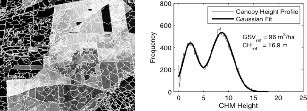
Figure 3.
randomForest out-of-bag GSV and CH estimates for pine stands based on stand-level ALS canopy structure indices versus in situ GSV and CH.
Figure 3.
randomForest out-of-bag GSV and CH estimates for pine stands based on stand-level ALS canopy structure indices versus in situ GSV and CH.
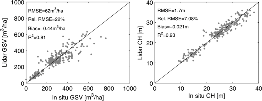
Figure 4.
randomForest predictor importance ranking for the ALS-based retrieval of GSV and CH.
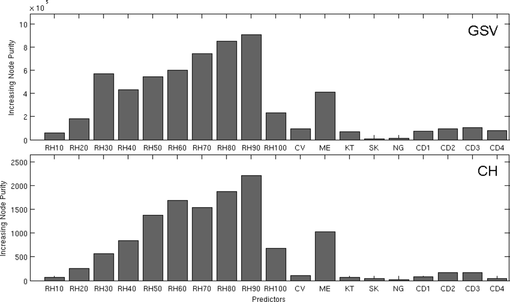
Figure 5.
Allometric relationship between GSV and CH for radiata pine stands.

Figure 6.
Estimates of GSV and CH obtained through fusion of multi-temporal dual-polarization ALOS PALSAR intensities and coherence and Landsat ETM+ data versus (1) Lidar estimates of GSV and CH for segments derived from the CHM (grey dots) and (2) in situ measurements of CH and GSV (black dots).
Figure 6.
Estimates of GSV and CH obtained through fusion of multi-temporal dual-polarization ALOS PALSAR intensities and coherence and Landsat ETM+ data versus (1) Lidar estimates of GSV and CH for segments derived from the CHM (grey dots) and (2) in situ measurements of CH and GSV (black dots).

Figure 7.
CH retrieval accuracy when using different combinations of the ALOS and Landsat data as predictors in randomForest. FBS, FBD and ETM stand for FBS intensity, FBD intensity and the Landsat data, respectively. FBDi and FBSi/FBDi denote the cases where intensities and coherences were used jointly. The white bars show the retrieval error when comparing the PALSAR/Landsat OOB against the ALS predictions. The grey bars refer to the comparison of the ALOS/Landsat predictions for the inventory polygons and the corresponding in situ measurements.

Figure 8.
randomForest predictor importance ranking for the retrieval of CH using all ALOS PALSAR imagery available at test site 2.
Figure 8.
randomForest predictor importance ranking for the retrieval of CH using all ALOS PALSAR imagery available at test site 2.

Figure 9.
Multi-temporal consistency of HH/HV intensity and repeat-pass coherence at test site 2. Each circle represents the average intensity or coherence for a forest segment in two images. The dashed lines indicate the dynamic range, δ, for each image with the 5th and 95th percentiles.
Figure 9.
Multi-temporal consistency of HH/HV intensity and repeat-pass coherence at test site 2. Each circle represents the average intensity or coherence for a forest segment in two images. The dashed lines indicate the dynamic range, δ, for each image with the 5th and 95th percentiles.

Figure 10.
Comparison of the per-segment CH predictions at test site 2 when using multi-temporal PALSAR FBD/FBS intensities with (ordinate) or without (abscissa) repeat-pass coherence as predictor layers in randomForest.
Figure 10.
Comparison of the per-segment CH predictions at test site 2 when using multi-temporal PALSAR FBD/FBS intensities with (ordinate) or without (abscissa) repeat-pass coherence as predictor layers in randomForest.
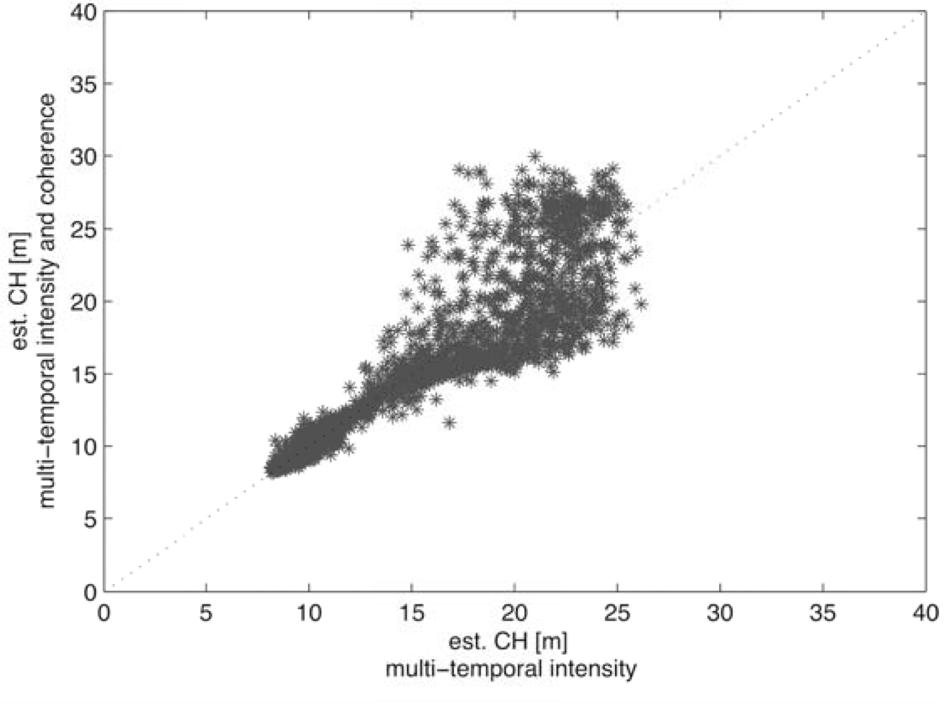
Figure 11.
Effect of ALS sampling density on the retrieval performance when extrapolating from 600m wide ALS transects to entire ALOS frames using multi-temporal intensities, repeat-pass coherence and one Landsat ETM+ optical scene.
Figure 11.
Effect of ALS sampling density on the retrieval performance when extrapolating from 600m wide ALS transects to entire ALOS frames using multi-temporal intensities, repeat-pass coherence and one Landsat ETM+ optical scene.

| Mean/SD | Range | |
|---|---|---|
| Canopy Height | 24/7 m | 8–39 m |
| Basal Area | 33/10 m2/ha | 13–77 m2/ha |
| Relative Stocking | 70/15% | 26–100% |
| Growing Stock Volume | 276/140 m3/ha | 37–768 m3/ha |
| Stand Size | 6.3/10 ha | 1–120 ha |
Table 2.
Properties of forest in inventory stands (FID) and segments derived from the ALS CHM (CH and GSV estimates from ALS) and the ALOS SAR/InSAR imagery available at each test site. PALSAR acquisitions for which the weather stations in Concepcion, Temuco or Curico reported rainfall (>1 mm) in the two days prior to the sensor overpasses are marked with superscript indices ‘c’, ‘t’ and ‘u’, respectively.
| Test Site | Slope (Mean/SD) | CH and GSV (mean/SD) | PALSAR Data | Coherence (Bn) | |
|---|---|---|---|---|---|
| Date | Mode | ||||
| 1 | 16/9° | CHFID: 29/11 m CHALS: 25/9 m GSVFID: 386/198 m3/ha GSVALS: 316/152 m3/ha | 10 Jul. | FBD | 10 Jul. & 10 Oct. (503 m) 10 Oct. & 25 Nov. (304 m) |
| 10 Oct. | FBD | ||||
| 7 Jan. | FBS | ||||
| 25 Nov. | FBS | ||||
| 11 Dec. | FBStc | ||||
| 2 | 2.6/5° | CHFID: 19/4 m CHALS: 17/6 m GSVFID: 172/70 m3/ha GSVALS: 154/98 m3/ha | 5 Jul. | FBDtc | 5 Jul. & 5 Oct. (597 m) 5 Oct. & 20 Nov. (214 m) 17 Feb. & 4 Apr. (567 m) 4 Apr. & 5 Jul. (320 m) |
| 5 Oct. | FBD | ||||
| 17 Feb. | FBStcu | ||||
| 4 Apr. | FBS | ||||
| 20 Nov. | FBS | ||||
| 3 | 6.5/4° | CHFID: 21/3 m | 17 Jul. | FBDtcu | |
| CHALS: 16/6 m | 1 Sep. | FBD | 17 Jul. & 1 Sep. (42 m) | ||
| GSVFID: 172/53 m3/ha | 1 Mar. | FBS | 1 Sep. & 2 Dec. (887 m) | ||
| GSVALS: 144/102 m3/ha | 2 Dec. | FBS | |||
Table 3.
CH and GSV retrieval error when using multi-temporal PALSAR SAR/INSAR as well as Landsat data as predictors in randomForest and ALS-based GSV and CH estimates as response variables. The accuracies refer to the comparison with (1) ALS-based estimates of CH and GSV and (2) the inventory data (FID).
| Test Site | Retrieval Error | ALS | FID | ||
|---|---|---|---|---|---|
| GSV | CH | GSV | CH | ||
| 1 | RMSE | 89.6 | 4.1 | 87.2 | 3.72 |
| RMSEr | 28.3 | 16.5 | 22.6 | 12.9 | |
| R2 | 0.79 | 0.82 | 0.72 | 0.76 | |
| Bias | 0.06 | 0.01 | −15.0 | −0.93 | |
| 2 | RMSE | 43.9 | 2.53 | 25.8 | 1.80 |
| RMSEr | 28.5 | 15.0 | 15.0 | 9.7 | |
| R2 | 0.81 | 0.82 | 0.87 | 0.86 | |
| Bias | 0.37 | 0.1 | −9.4 | −1.0 | |
| 3 | RMSE | 42.6 | 2.4 | 43.8 | 1.8 |
| RMSEr | 29.6 | 15.6 | 25.5 | 8.5 | |
| R2 | 0.83 | 0.86 | 0.87 | 0.86 | |
| Bias | −0.1 | 0.01 | 20 | −0.51 | |
Share and Cite
MDPI and ACS Style
Cartus, O.; Kellndorfer, J.; Rombach, M.; Walker, W. Mapping Canopy Height and Growing Stock Volume Using Airborne Lidar, ALOS PALSAR and Landsat ETM+. Remote Sens. 2012, 4, 3320-3345. https://doi.org/10.3390/rs4113320
AMA Style
Cartus O, Kellndorfer J, Rombach M, Walker W. Mapping Canopy Height and Growing Stock Volume Using Airborne Lidar, ALOS PALSAR and Landsat ETM+. Remote Sensing. 2012; 4(11):3320-3345. https://doi.org/10.3390/rs4113320
Chicago/Turabian StyleCartus, Oliver, Josef Kellndorfer, Markus Rombach, and Wayne Walker. 2012. "Mapping Canopy Height and Growing Stock Volume Using Airborne Lidar, ALOS PALSAR and Landsat ETM+" Remote Sensing 4, no. 11: 3320-3345. https://doi.org/10.3390/rs4113320