Improving Wishart Classification of Polarimetric SAR Data Using the Hopfield Neural Network Optimization Approach


Abstract
:1. Introduction
2. Hopfield Neural Network Optimization Process
2.1. Decomposition and Wishart Classifier
- The polarimetric scattering information may be represented for each image pixel by the Pauli scattering vector . Hence, is the Hermitian product of the target vector of the one-look ith pixel. PolSAR data need to be multilook processed for speckle reduction by averaging n neighboring pixels. The coherency matrix is then obtained as,where the superscripts * and t denote the complex conjugate and matrix transposition, respectively.
- From the coherency matrices, we apply the H/ᾱ decomposition process as a refined scheme to parameterize polarimetric scattering problems. The scattering entropy, H, is a key parameter in determining the degree of statistical disorder, in such a way that H = 0 indicates the presence of a single scattering mechanism and H = 1 results when three scattering mechanisms with the same power are present in the resolution cell. The angle ᾱ characterizes the scattering mechanism as proposed in [8–10].
- The next step is to classify the PolSAR data into nine classes in the H/ᾱ plane, although zone three never contains pixels. These classes include different types of scattering mechanisms present in the scene, such as vegetation (grass, bushes), water surface (ocean or lakes) or city block areas. Section 3.3 includes a description and discussion about the content of these classes.
- Hence, the classification process results in eight valid zones or clusters, where each class is identified as wj or j, i.e., in our approach j varies from one to nine. Then, we compute the initial cluster center of coherency matrices for all pixels belonging to each zone (class wj) according to the number of pixels nj belonging to the class wj as follows,
- Compute the distance measure for each pixel i characterized by its coherence matrix 〈T〉i to the cluster center as follows,
- Assign the pixel to the class with the minimum distance,
- Verify if the termination criterion is met, otherwise set t = t + 1 and return to Step 1. The termination criterion is set to a prefixed number of iterations tmax. Nevertheless, the criteria that we adopt are the following: assuming that at each iteration t we have pixels belonging to the class wj and at the next iteration t + 1 the pixels belonging to the same class are , if the relative difference between both quantities is below a certain percentage, then the process also stops. We experimented with thresholds between ±0.5% and ±5%.
2.2. Cluster Separation Measures
- The dispersion within clusters (Dii): The Dii is defined as the averaged distance between all the pixels within the cluster wi to the cluster center Vi. It measures the compactness of cluster wi and is given by,where the large Dii indicates the dispersion of the pixels into the cluster.
- The distance between two clusters (Dij) is defined as,where the large Dij values indicate the high separation of these two clusters.
- The cluster separability (Rij) involves two clusters and is defined as,a small Rij value indicates that these two clusters are well separated; Rij is the Davies-Bouldin index [16] in classical clustering approaches, here adapted to PolSAR data classification. This quantity measures the quality of the partition, i.e., the clustering quality.
2.3. The Hopfield Neural Network for Improving the Wishart Classification
2.3.1. Preliminary Considerations and Network Architecture
- How can we achieve that a pixel changes its current label so that it is classified as belonging to a different class?
- How can we achieve that a pixel does not change its label when its neighbors have identical labels as the label of the pixel under analysis?
- How can we achieve maximum cluster separability?
- When can we consider that no more changes are required?
2.3.2. Dynamics of the Hopfield Neural Network
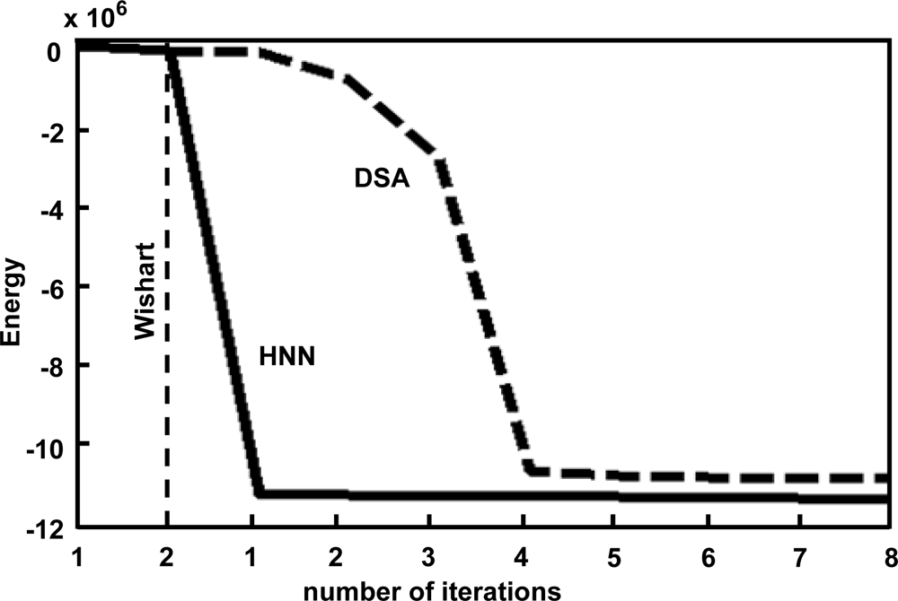
2.3.3. Energy Definition
2.3.4. Derivation of the Connection Weights and External Inputs for the HNN
2.3.5. Summary of the HNN-Based Image Classifier
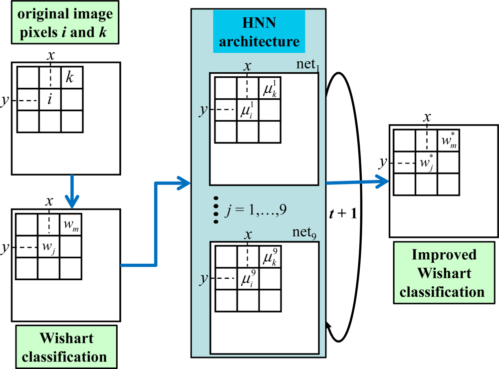
- Initialization: create a network netj for each cluster wj. For each netj create a node i at each pixel location (x,y) from the image to be classified; t = 0 (iteration number); load each node with the state value , i.e. the support provided by the Wishart-based classifier, Equation (9); compute and through Equation (20); set ε = 0.01 (a constant to accelerate the convergence); tmax = 4 (maximum number of iterations allowed, see Section 3.2); set the constant values as follows: Li = 1; β = 3.38; dt = 10−3. Define nc as the number of nodes that change their state values at each iteration. The iterations in this discrete approach represent the time evolution involved in Equation (12).
- HNN process: set t = t + 1 and nc = 0; for each node i in netj compute using the Runge-Kutta method and update , both according to Equation (12) and ifthen nc = nc + 1; when all nodes i have been updated, if nc ≠ 0 and t < tmax then go to Step 2 (new iteration), else stop.
- Outputs: updated for each node; it is the degree of support for the cluster wj, see Figure 1. The node i is classified as belonging to the cluster with the greatest degree.
3. Experimental Results
3.1. Design of a Test Strategy
3.2. Results
3.3. Discussion
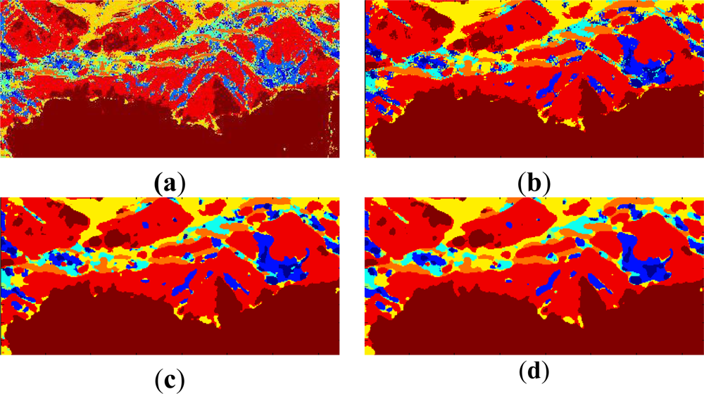
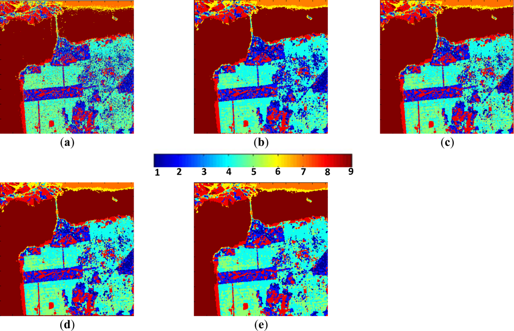
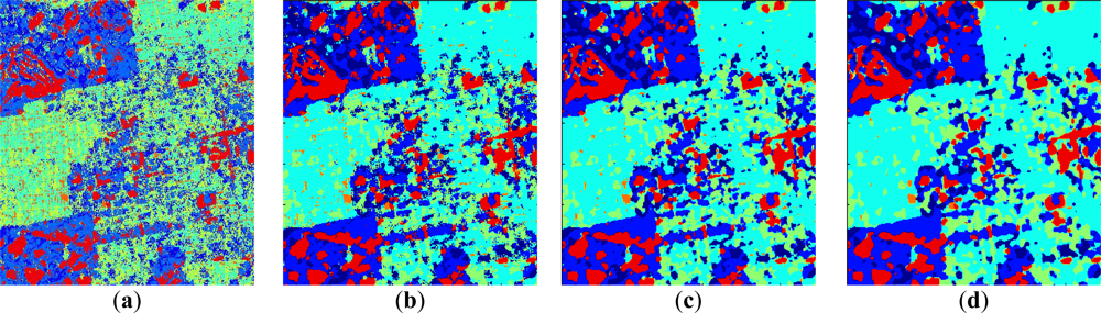
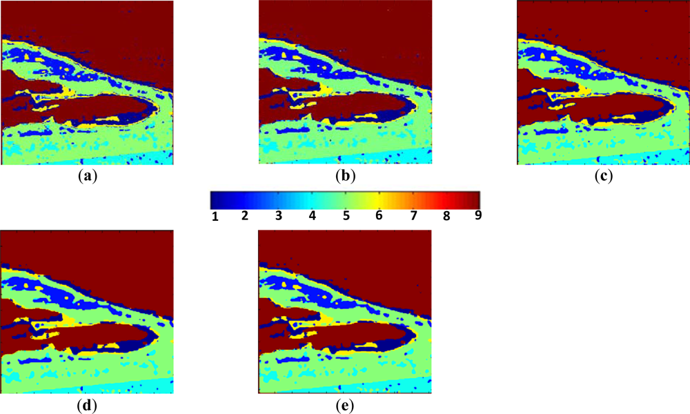
- The low entropy vegetation consisting of grass and bushes belonging to the cluster w2 has been clearly homogenized, this is because there are many pixels belonging to w4 in these areas re-classified as belonging to w2.
- Also, in accordance with [13], the areas with abundant city blocks display medium entropy scattering. We have homogenized the city block areas removing pixels in areas that belong to clusters w1 and w2, so that they are re-classified as belonging to w4 and w5 as expected.
- Some structures inside other broader regions are correctly isolated. This occurs in the rectangular area corresponding to a park, where the internal structures with high entropy are clearly visible [33].
- Additionally, the homogenization effect can be considered as a mechanism for speckle noise reduction during the classification phase, avoiding the early filtering for classification tasks.
4. Conclusions
Acknowledgments
References
- Lee, J.S.; Grunes, M.R.; Pottier, E.; Ferro-Famil, L. Unsupervised terrain classification preserving scattering characteristics. IEEE Trans. Geosci. Remote Sens 2004, 42, 722–731. [Google Scholar]
- Lee, J.S.; Pottier, E. Polarimetric Radar Imaging: From Basics to Applications, 1st ed.; CRC Press: Boca Raton, FL, USA, 2009. [Google Scholar]
- Ferro-Famil, L.; Pottier, E.; Lee, J.S. Unsupervised classification of multifrequency and fully polarimetric SAR images based on the H/A/Alpha-Whisart classifier. IEEE Trans. Gosci. Remote Sens 2001, 39, 2332–2342. [Google Scholar]
- Benz, U.; Pottier, E. Object Based Analysis of Polarimetric SAR Data in alpha-Entropy-Anisotropy Decomposition Using Fuzzy Classification by eCognition. Proceedings of IEEE Int. Geoscience and Remote Sensing Symposium (IGARSS ’01), Sydney, Australia, 9–13 July 2001; pp. 1427–1429.
- Hara, Y.; Atkins, R.G.; Yueh, S.H.; Shin, R.T.; Kong, J.A. Application of neural networks to radar image classification. IEEE Trans. Geosci. Remote Sens 1994, 32, 100–110. [Google Scholar]
- Du, L.; Lee, J.S. Fuzzy classification of earth terrain covers using complex polarimetric SAR data. Int. J. Remote Sens 1996, 17, 809–826. [Google Scholar]
- Grandi, G.D.; Lucas, R.M.; Kropacek, J. Analysis by wavelet frames of spatial statistics in SAR data for characterizing structural properties of forests. IEEE Trans. Geosci. Remote Sens 2009, 47, 494–507. [Google Scholar]
- Cloude, S.R.; Pottier, E. A review of target decomposition theorems in radar polarimetry. IEEE Trans. Geosci. Remote Sens 1996, 34, 498–518. [Google Scholar]
- Cloude, S.R.; Pottier, E. Application of the H/A/a polarimetric decomposition theorem for land classification. Proc. SPIE 1997, 3120, 132–143. [Google Scholar]
- Cloude, S.R.; Pottier, E. An entropy based classification scheme for land applications of PolSAR. IEEE Trans. Geosci. Remote Sens 1997, 35, 68–78. [Google Scholar]
- Pottier, E.; Lee, J.S. Unsupervised Classification Scheme of Pol-SAR Images Based on the Complex Wishart Distribution and the H/A/α Polarimetric Decomposition Theorem. Proceedings of EUSAR, Munich, Germany, 23–25 May 2000; pp. 265–268.
- Lee, J.S.; Grunes, M.R.; Kwok, R. Classification of multi-look polarimetric SAR imagery based on complex Wishart distribution. Int. J. Remote Sens 1994, 15, 2299–2311. [Google Scholar]
- Lee, J.S.; Grunes, M.R.; Ainsworth, T.; Du, L.J.; Schuler, D.; Cloude, S. Unsupervised classification using polarimetric decomposition and the complex Wishart classifier. IEEE Trans. Geosci. Remote Sens 1999, 37, 2249–2258. [Google Scholar]
- Hopfield, J.J.; Tank, D.W. Neural computation of decisions in optimization problems. Biol. Cyber 1985, 52, 141–152. [Google Scholar]
- Hopfield, J.J.; Tank, D.W. Computing with neural circuits: A model. Science 1986, 233, 625–633. [Google Scholar]
- Davies, D.L.; Bouldin, D.W. A cluster separation measure. IEEE Trans. Pattern Anal. Machine Intell 1979, 1, 224–227. [Google Scholar]
- Wang, D. The time dimension for scene analysis. IEEE Trans. Neural Netw 2005, 16, 1401–1426. [Google Scholar]
- Sánchez-Lladó, F.J.; Pajares, G.; López-Martínez, C. Improving the Wishart synthetic aperture radar image classifications through deterministic simulated annealing. ISPRS J. Photogramm 2011, 66, 845–857. [Google Scholar]
- Joya, G.; Atencia, M.A.; Sandoval, F. Hopfield neural networks for optimization: Study of the different dynamics. Neurocomputing 2002, 43, 219–237. [Google Scholar]
- Haykin, S. Neural Networks: A Comprehensive Foundation; Macmillan College Publishing Co.: New York, NY, USA, 1994. [Google Scholar]
- Qiao, H.; Peng, J.; Xu, Z.B. Nonlinear Measures: A new approach to exponential stability analysis for Hopfield-type neural networks. IEEE Trans. Neural Netw 2001, 12, 360–370. [Google Scholar]
- Yu, S.S.; Tsai, W.H. Relaxation by the Hopfield Neural Network. Pattern Recog 1992, 25, 197–209. [Google Scholar]
- Kasetkasem, T.; Varshney, P.K. An image change detection algorithm based on Markov Random field models. IEEE Trans. Geosci. Remote Sens 2002, 40, 1815–1823. [Google Scholar]
- Starink, J.P.; Backer, E. Finding point correspondences using simulated annealing. Pattern Recog 1995, 28, 231–240. [Google Scholar]
- van Laarhoven, P.M.J.; Aarts, E.H.L. Simulated Annealing: Theory and Applications; Kluwer Academic Publishers: Boston, MA, USA, 1988. [Google Scholar]
- Hajek, B. Cooling schedules for optimal annealing. Math. Operation Res 1988, 13, 311–329. [Google Scholar]
- Kosko, B. Neural Networks and Fuzzy Systems: A Dynamical Systems Approach to Machine Intelligence; Prentice-Hall: Englewood Cliffs, NJ, USA, 1992. [Google Scholar]
- Cohen, M.A.; Grossberg, S.G. Absolute stability of global pattern formation and parallel memory storage by competitive neural networks. IEEE Trans. Syst. Man Cyber 1983, 13, 815–826. [Google Scholar]
- Lee, D.L.; Chuang, T.C. Designing asymmetric Hopfield-type associative memory with higher order Hamming stability. IEEE Trans. Neural Netw 2005, 16, 1464–1476. [Google Scholar]
- Zhao, Z.Q. A novel modular neural network for imbalanced classification problems. Pattern Recog. Lett 2009, 30, 783–788. [Google Scholar]
- Müezzinoglu, M.K.; Güzelis, C.; Zurada, J.M. An energy function-based design method for discrete Hopfield associative memory with attractive fixed points. IEEE Trans. Neural Netw 2005, 16, 370–378. [Google Scholar]
- Idbraim, S.; Aboutajdine, D.; Mammass, D.; Ducrot, D. Classification of Remote Sensing Imaging by an ICM Method with Constraints: Application in Land Cover Cartography. Proceedings of IEEE International Conference on Multimedia Computing and Systems (ICMCS’09), Ouarzazate, Morocco, 2–4 April 2009; pp. 472–477.
- Google Earth. The Google Earth Product Family. Available online: http://www.google.es/intl/es/earth/index.html (accessed on 20 September 2012).
- Turner, D.; Woodhouse, I.H. An icon-based synoptic visualization of fully polarimetric radar data. Remote Sens 2012, 4, 648–660. [Google Scholar]
- Cui, Y.; Yamaguchi, Y.; Yang, J.; Park, S-E.; Kobayashi, H.; Singh, G. Three-component power decomposition for polarimetric SAR data based on adaptive volume scatter modeling. Remote Sens 2012, 4, 1559–1572. [Google Scholar]


| Wishart | |||||||
|---|---|---|---|---|---|---|---|
| # of iterations | 1 | 2 | 3 | 4 | 5 | 6 | 7 |
| R̄ | 91.8 | 78.3 | 116.1 | 145.2 | 112.8 | 93.0 | 106.6 |
| R̄ | # of iterations | ||||||||
|---|---|---|---|---|---|---|---|---|---|
| 1 | 2 | 3 | 4 | 5 | 6 | 7 | 8 | ||
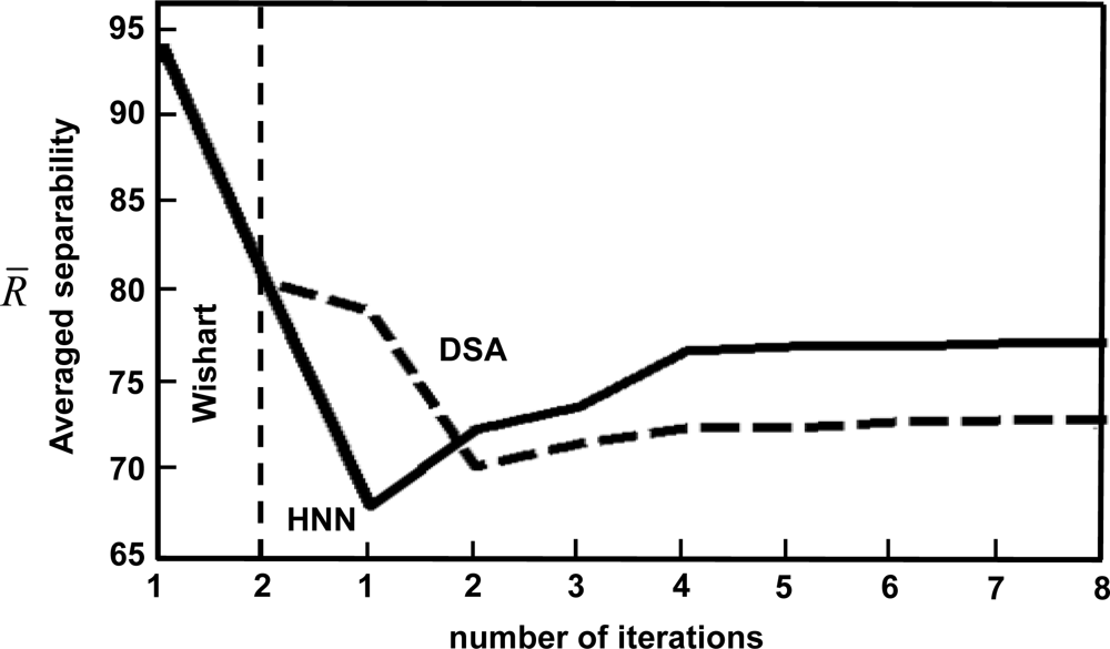
| HNN | 65.5 | 69.9 | 71.2 | 74.3 | 74.3 | 74.6 | 74.8 | 74.9 | |
| DSA | 76.6 | 67.8 | 69.1 | 70.0 | 70.0 | 70.3 | 70.4 | 70.5 | |
| HNN | 135.8 | 183.7 | 189.2 | 192.1 | 192.9 | 193.7 | 194.6 | 196.2 | |
| DSA | 177.3 | 158.9 | 182.2 | 188.1 | 190.5 | 197.1 | 199.4 | 202.6 | |
| HNN | 301.2 | 444.1 | 445.3 | 449.1 | 449.9 | 452.2 | 455.3 | 458.1 | |
| DSA | 354.3 | 321.4 | 432.6 | 488.4 | 489.9 | 493.2 | 495.1 | 497.3 | |
| Wishart | HNN | DSA | ICM | MAJ | |
|---|---|---|---|---|---|
| R̄ | 78.3 | 67.7 | 67.8 | 71.5 | 93.1 |
| H̄ | 0.354 | 0.286 | 0.291 | 0.192 | 0.184 |
| Average CPU times (minutes/iteration) | 3.01 | 2.02 | 2.31 | 2.28 | 2.35 |
| Wishart | HNN | DSA | ICM | MAJ | |
|---|---|---|---|---|---|
| R̄ | 24.3 | 22.4 | 22.4 | 24.2 | 25.9 |
| H̄ | 0.121 | 0.088 | 0.089 | 0.081 | 0.083 |
| Average CPU times (minutes/iteration) | 1.10 | 0.76 | 0.77 | 0.75 | 0.81 |
Share and Cite
Pajares, G.; López-Martínez, C.; Sánchez-Lladó, F.J.; Molina, Í. Improving Wishart Classification of Polarimetric SAR Data Using the Hopfield Neural Network Optimization Approach. Remote Sens. 2012, 4, 3571-3595. https://doi.org/10.3390/rs4113571
Pajares G, López-Martínez C, Sánchez-Lladó FJ, Molina Í. Improving Wishart Classification of Polarimetric SAR Data Using the Hopfield Neural Network Optimization Approach. Remote Sensing. 2012; 4(11):3571-3595. https://doi.org/10.3390/rs4113571
Chicago/Turabian StylePajares, Gonzalo, Carlos López-Martínez, F. Javier Sánchez-Lladó, and Íñigo Molina. 2012. "Improving Wishart Classification of Polarimetric SAR Data Using the Hopfield Neural Network Optimization Approach" Remote Sensing 4, no. 11: 3571-3595. https://doi.org/10.3390/rs4113571