Article

Modeling Species Distribution Using Niche-Based Proxies Derived from Composite Bioclimatic Variables and MODIS NDVI

1
Department of Geography, University of Erlangen-Nuremberg, Kochstr. 4/4, D-91054 Erlangen, Germany
2
Department of Biological Sciences, Murray State University, Murray, KY 42071, USA
3
GIS and Remote Sensing Unit, Department of Biodiversity and Molecular Ecology, Fondazione Edmund Mach, Research and Innovation Centre, Via E. Mach 1, I-38010 S. Michele all’Adige, Italy
*
Author to whom correspondence should be addressed.
Remote Sens. 2012, 4(7), 2057-2075; https://doi.org/10.3390/rs4072057
Submission received: 20 May 2012 / Revised: 30 June 2012 / Accepted: 2 July 2012 / Published: 9 July 2012
(This article belongs to the Special Issue Remote Sensing of Biological Diversity)

Abstract

:
Vegetation mapping based on niche theory has proven useful in understanding the rules governing species assembly at various spatial scales. Remote-sensing derived distribution maps depicting occurrences of target species are frequently based on biophysical and biochemical properties of species. However, environmental conditions, such as climatic variables, also affect spectral signals simultaneously. Further, climatic variables are the major drivers of species distribution at macroscales. Therefore, the objective of this study is to determine if species distribution can be modeled using an indirect link to climate and remote sensing data (MODIS NDVI time series). We used plant occurrence data in the US states of North Carolina and South Carolina and 19 climatic variables to generate floristic and climatic gradients using principal component analysis, then we further modeled the correlations between floristic gradients and NDVI using Partial Least Square regression. We found strong statistical relationship between species distribution and NDVI time series in a region where clear floristic and climatic gradients exist. If this precondition is given, the use of niche-based proxies may be suitable for predictive modeling of species distributions at regional scales. This indirect estimation of vegetation patterns may be a viable alternative to mapping approaches using biochemistry-driven spectral signature of species.

Graphical Abstract

1. Introduction

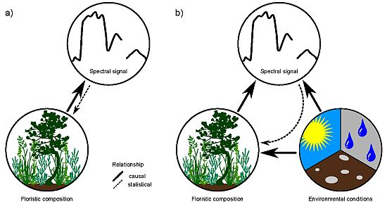
Remote-sensing approaches for mapping individual species or plant assemblages frequently rely on the biochemistry of the target species/assemblage [13]. Together with biophysical properties, plant biochemistry is directly responsible for the spectral signature of vegetation. For vegetation mapping, this relationship is inverted and the spectral signal is used to draw conclusions of the presence of a species or assemblage (see Figure 1(a)). A unique biochemistry of species along with phenological and structural characteristics may enable a discrimination of vegetation, but is inevitable for a reliable mapping result. Problems may arise if different species feature a similar spectral response, which is a common phenomenon in remote sensing [4,5]. A unique biochemistry and spectral signal is considered neither in the biological definition of a species, nor in the ecological classification of plant assemblages [6]. Further, species-specific biochemistry and spectral signal show a large spatio-temporal variation due to site conditions and other external influences [4]. This hampers a direct inversion of the relationship towards a quantification of the floristic composition and makes the direct mapping or classification of vegetation with remote-sensing approaches very challenging. However, mapping and modeling species distribution using remote sensors is still desirable. In particular at global and regional scales, where ground-based mapping is inefficient, remote sensing may be a practical alternative approach for vegetation mapping.
Environmental conditions, such as climate, also affect the biophysical and biochemical properties of species and hence influence their spectral signal [4,7]. Environmental conditions, especially temperature and precipitation, are further major determinants of species distribution at macroscales [8,9]. Indirect causal relationships between species distribution/occurrences derived from the spectral response of the environmental conditions, which define the ecological niche of the species, may hence be promising (Figure 1(b)). This is because the spectral signal is a direct reflection of environmental properties, thus representing a powerful proxy for floristic composition in species distribution mapping and modeling.
Therefore, we address in this paper the question whether we are able to model the floristic composition based on the ecological requirements of plant species and the spectral response to the corresponding environmental conditions. Our goal is to integrate environmental factors/climatic variables, floristic composition, and spectral information into a causal framework which has not been investigated before. We expect that the outcome of this study might have significant implications to remote sensing of floristic vegetation patterns.
The fundamental range of tolerance of a species, which is a result of limiting factors of the environment, is a critical determinant of the resultant distribution pattern [1013]. Limiting factors are typically related to climate properties, such as temperature and water availability, at a broad geographical scale. At a finer scale, resource factors/gradients, including nutrients, amount of light energy for plants, food for animals, and moisture level, driven by topographical variations and habitat types, are the main driving forces for shaping the patterns of species distribution. Additionally, natural and anthropogenic disturbances affect species distribution at various spatial scales.
From a theoretical point of view, species distribution at difference spatial scales closely ties to the fundamental and realized niche concepts proposed by Hutchinson [14]. According to him, the fundamental niche refers to abiotic conditions in which a species can persist and maintain a stable population, whereas the realized niche describes the environmental conditions in which a species is able to survive and reproduce in the presence of biotic interactions, such as competition, predation, and symbiosis. The focal part of both niche concepts suggests that ecological niches function as an ecophysiological constraint on species distribution. It is expected that individuals living under the conditions outside the niche will not be able to maintain a stable population under selection pressure, thus a decline in population size can become real and inevitable.
It is fairly common in ecological studies that direct or indirect relations between measurable and nearly unmeasurable variables are contemplated for seeking causal driving factors for species distribution and abundance. For instance, ecological variables based on field sampling are necessary inputs for niche models. However, many of these variables are impossible to measure in reality. To overcome this problem, ecologists usually rely on information derived from available maps, such as digital elevation models to obtain topographical variables to develop predictive models for species occurrence [15,16]. Climatic data are also collected or interpolated from climate stations for a large spatial scale modeling such as the bioclimatic envelope models [1719]. Similarly, remotely-sensed reflectance data are also employed as a good proxy for floristic composition/pattern recognition in vegetation studies [2021]. However, remote sensing data have not been used frequently in species distribution modeling, even though they can provide greater coverage in space and time.
More recently, there is an increasing trend in using remote sensing information based, e.g., on various spectral indices recorded from airborne or space-borne sensors as predictor variables in species distribution modeling [2226]. A few studies have shown that niche models developed by incorporating remotely-sensed predictors are more robust; in particular, these data can improve the prediction accuracy and tend to refine mapped distribution of species and habitats, compared with climatic/topographical variables-only models [2729]. Remotely-sensed indices, such as NDVI, may hence provide the opportunity to complement or improve niche models based on climate data alone. This is even more evident considering the fact that many climatic variables are the results of interpolation from potentially sparse weather stations and derived from different statistical approaches [30]. Therefore, in this paper, we attempt to model the floristic composition of vegetation using an indirect link to climate and remote sensing data and we further contemplate the causal linkages between climate, phenology detected by remote sensors, and floristic gradients expressed by principal components.

2. Material and Methods

2.1. Study Area

We chose the two states of North Carolina and South Carolina in the United States as our entire study area, due to the enormous ecological and biological diversity in the region. The two states contain a wide range of land cover types, including coastal lowlands, large river floodplain forests, rolling plains and plateaus, and forested mountains. There are four EPA level III ecoregions ( http://www.epa.gov/wed/pages/ecoregions/level_iii.htm#Ecoregions) in the area including Piedmont (55 counties), a part of temperate hardwood forests found in the eastern North America; Middle Atlantic Coastal Plain (35 counties), containing mostly swamps and salt marshes; Southeastern Plains (35 counties), a mosaic of forest woodland and pasture/cropland; and Blue Ridge (20 counties), including Appalachian oak forests, northern hardwood forests and spruce-fir forests. Detailed ecoregion maps including all counties in the two states can be found in He et al. [21].

2.2. Floristic Data

The floristic composition of the vegetation in North and South Carolina was extracted on a county base from the USDA plant database ( http://plants.usda.gov/java/). The database listed 3,151 species with an occurrence in at least one county. No data were available for the Alamance County in North Carolina. This county was hence excluded from all analyses, reducing the data set to a total of 145 counties. The compiled floristic data consisted of binary records of species presences and absences. No information on species cover fractions, dominances, or abundances was given in this dataset. The spectral signal of vegetation assemblages is dependent on species cover fractions as reflectance captured by remote sensors. A very weak direct relation between these binary floristic data and the actual spectral signal of the assemblages was hence expected.

2.3. Bioclimate Variables

At this regional scale, we assumed that climate is a major determinant of floristic patterns in North Carolina and South Carolina. We hence extracted 19 bioclimatic variables for each county from the BIOCLIM dataset ( http://www.worldclim.org/) (Table 1). These 19 bioclimatic variables were obtained from more than 4,000 weather stations between 1950 and 2000 [30]. The spatial resolution of the bioclimate data was 30 arc-seconds (∼1 km) and we calculated the means of each variable for each county.

2.4. MODIS-NDVI Time Series

Reflectance-derived vegetation indices have been widely used among ecologists to study compositional changes of vegetation under the changing climate at a large spatial scale. One of the most commonly used indices is the Normalized Difference Vegetation Index (NDVI), stating a ratio between red and near-infrared reflectance captured by satellite sensors [31,32]. NDVI metrics have been successfully used to estimate biomass and net primary productivity [33], because NDVI values are associated with the photosynthetically-active radiation of plant canopies [31,32,34].
The MODIS (Moderate-resolution Imaging Spectroradiometer) NDVI data used in this study have a spatial resolution of 250 meters and temporal resolution of 16 days. There are 23 time points for a whole year. We downloaded the 23 NDVI images for the year 2005 ( http://glcf.umiacs.umd.edu/data/ndvi). For areas covered by vegetation, the NDVI is strongly related to the phenological development and hence to the climatic conditions. The NDVI-values of each date were averaged to county-based values that were used for the subsequent analyses.

2.4. Statistical Analyses

We subjected the floristic data to a principal component analysis (PCA) to reduce its dimensionality. Binary records of species’ presence and absence (1 or 0) for each county were used as the original dataset for PCA. The resulting principal components (i.e., floristic gradients) comprise hierarchically large parts of the information content of the original data. The counties’ scores on the main principal components are a quantitative and continuous measure of the changing floristic composition according to Gleason’s continuum concept [35,36]. Counties with a similar floristic inventory feature similar scores on the floristic gradients, while dissimilar species show larger inter-distances in the PCA-space. We used the spatial distribution of PC-scores as the basis for all subsequent analyses.
The 19 climatic parameters used in this study are highly inter-correlated. This inter-correlation hampers any interpretation and analysis. We hence used a PCA of the climate data to eliminate the inter-correlation and to extract independent climatic gradients. Subsequently, we analyzed the loadings of the parameters on the PCs and identified for each PC a corresponding parameter to ease interpretation. These ‘master variables/descriptors’ were passed to the subsequent analyses.
We assumed causal relations between both climate and floristic patterns, as well as between climate and NDVI. In order to test whether these assumptions correspond to statistically significant relations, two sets of correlation analyses were used. First, we tested for correlations between the climatic master variables and floristic composition as expressed by the floristic gradients extracted by PCA. These analyses were used to evaluate the assumption that the distribution of floristic vegetation patterns in North Carolina and South Carolina is dependent on climatic conditions. In a second set of analyses we tested for significant correlations between the climatic variables and the NDVI pattern on different dates.
Finally, we tested the statistical relationship between the floristic gradients and the NDVI time series with regression analyses. To cope with the inter-correlation inherent to the NDVI data, we used Partial Least Squares regression (PLSR, [37]). This regression approach was originally developed in the field of chemometrics to analyze spectral data. It was subsequently adopted in remote sensing and has since then successfully been used in numerous studies targeting different vegetation properties (e.g., [6,3843]).
PLSR is basically a multivariate regression, including so-called latent vectors (LVs) as independent variables. These LVs are statistically independent linear combinations of the original variables (i.e., the inter-correlated NDVI time series). Contrary to the PCs in PCA, the LVs are generated under simultaneous consideration of both independent and the dependent (i.e., the floristic gradients) variables. Therefore, the LVs are optimized towards the explanation of the response variable and the model parsimony can be increased [37]. Model validation took place by 10-fold cross-validation. For each floristic gradient we built multiple models that included step-wise increasing numbers of LVs. To reduce the possibility of over-fitting and to optimize the trade-off between model fit and model parsimony, we selected the model with the number of LVs resulting in the smallest root mean squared error in validation (RMSEval). A backward selection approach (following [44]) was used to further refine this model and to reduce the set of NDVI dates to the time steps showing a stable and significant relation to the floristic pattern. The residuals of the final model for each floristic gradient were tested for spatial autocorrelation by calculating Moran’s i for increasing distance classes between county centroids.
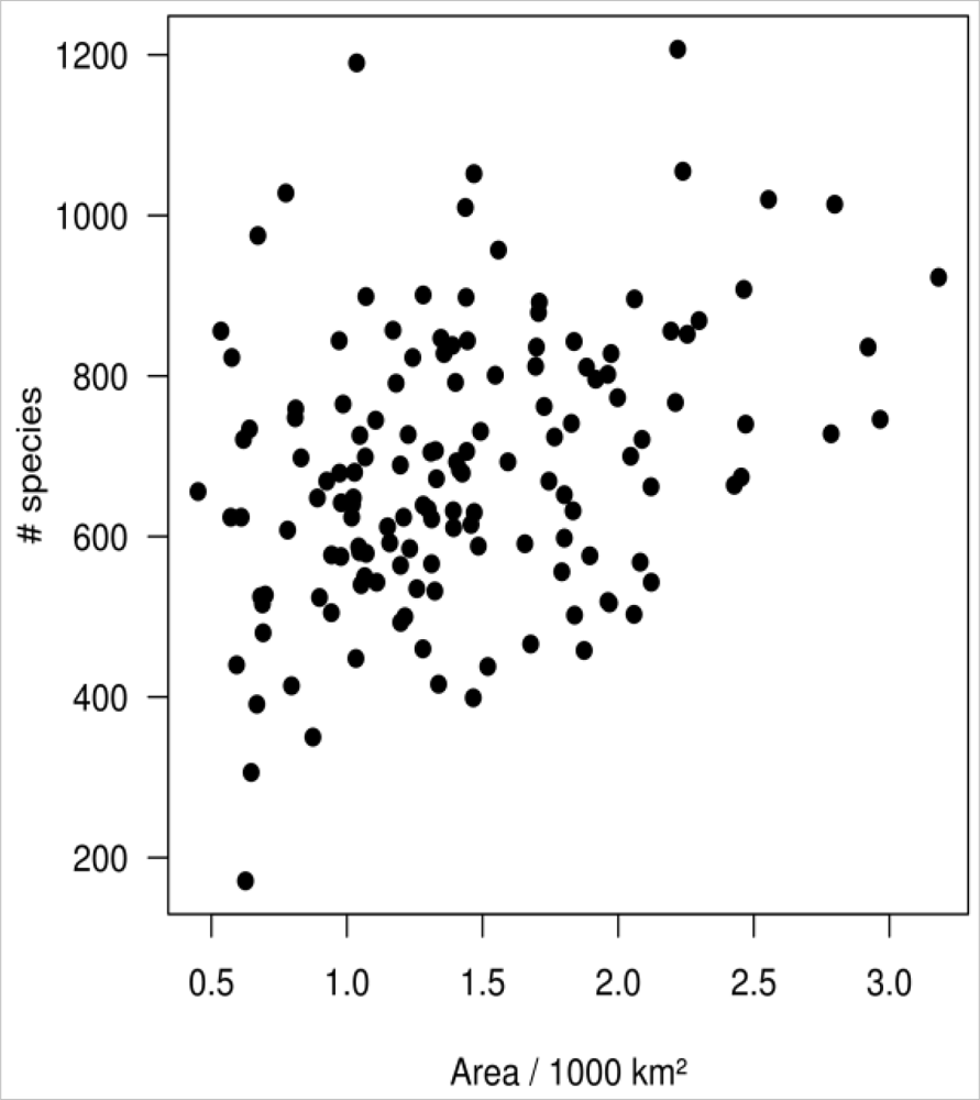
Unfortunately, all data used in this study are on a per-county basis. Apart from being not ecologically meaningful, this basis is likely to affect the results of the study, since the area of the counties is unequal (ranging from 450 to 3,180 km2). The unequal area may in particular affect the number of observed species per county which generally grows with increasing area. To test if such an area effect exists, we plotted the species-area curve and formally tested the relation using the Mantel test. Resemblance matrices were generated using Euclidian distance for both county area and species richness per county as the input for the Mantel test.

3. Results

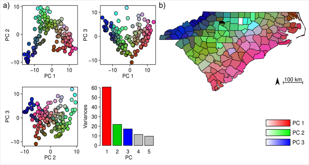
The PCA revealed three prominent floristic gradients in the vegetation data (Figure 2(a)). The spatial distribution of the PC scores (Figure 2(b)) showed that these gradients formed a clear spatial pattern, and floristic composition gradually changed from the coastline in the east to the mountains in the west. The cumulative variance explained by the first three PCs of floristic data was 55%. A weak relationship (Mantel test: r = 0.13, p = 0.006 from Monte-Carlo permutation test) was found between county area and species richness per county (Figure 3).
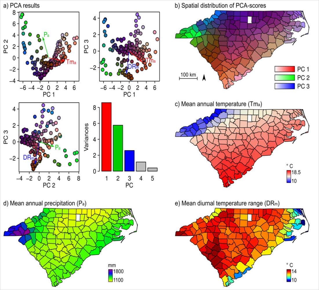
The PCA of the county-based bioclimate data revealed three strong climatic gradients (Figure 4(a)). The cumulative variance explained by the first three PCs was 50%. The analysis of the loadings showed that the main PCs represent a temperature gradient, a precipitation gradient, and a gradient from marine to continental climate. Three variables: mean annual temperature, annual precipitation, and mean diurnal temperature range were identified to represent these climatic gradients (Figure 4(c–e)).
We summarized the correlations between these three climatic variables and the floristic gradients. The first and second floristic gradients showed a highly significant correlation with the climatic variables. The 3rd PC of the floristic data was almost independent of climate (Table 2).
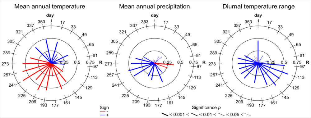
We also analyzed the correlations between the three climatic variables/composite PCs and the NDVI pattern on different dates (Figure 5). Strong correlations between Tma and the NDVI were observed throughout the year. However, the sign of the correlation coefficients changed from summer to winter and vice versa. In summer, colder temperatures were related to a high NDVI signal; in winter, the NDVI values increased with warmer temperatures. Further, we observed positive correlations between NDVI and both precipitation and diurnal temperature range.
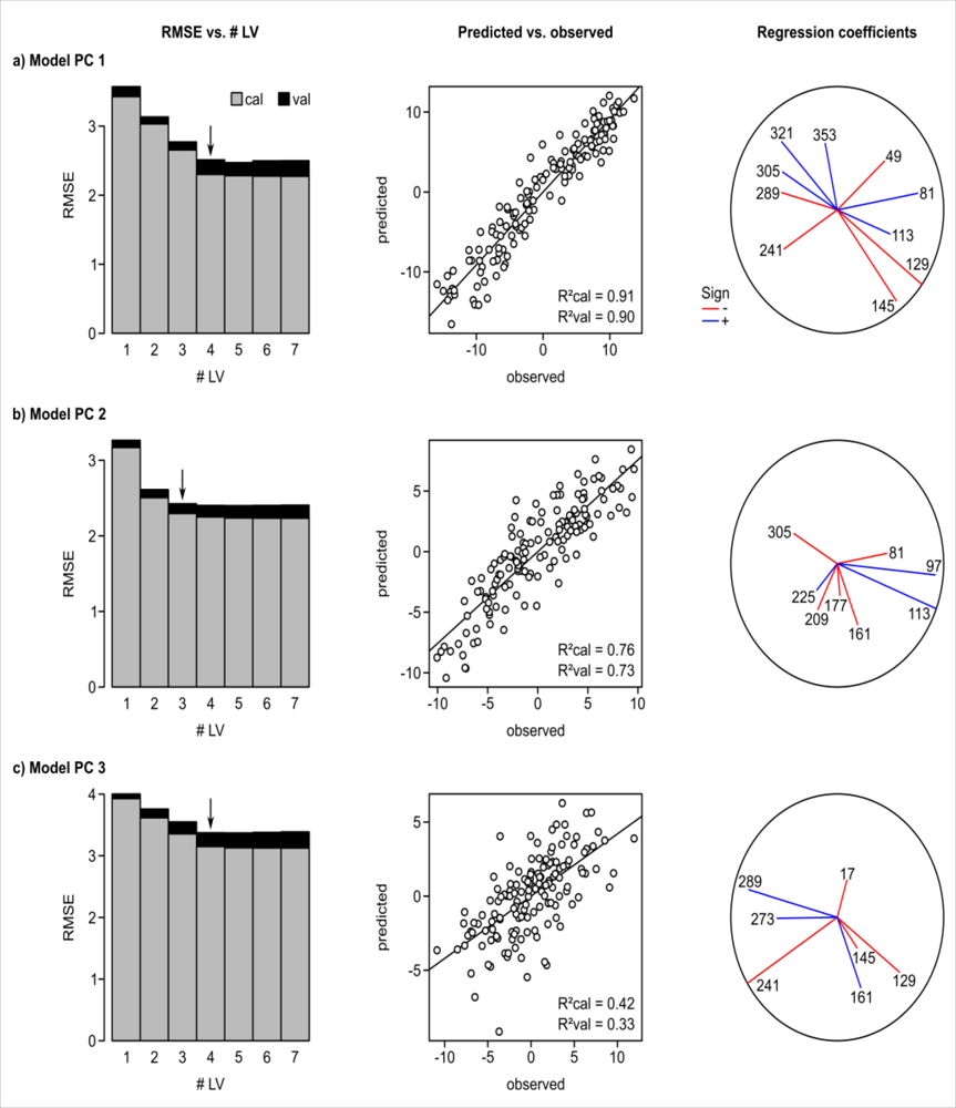
Lastly, we analyzed the relationship between floristic gradient and NDVI time series using PLSR. Results of the PLSR regressions between floristic gradients and NDVI time series are shown in Figure 6. The model for the main floristic gradient (PC1) resulted in R2 = 0.9, the model for the 2nd PC in R2 = 0.73, and the model for the 3rd PC in R2 = 0.33 in cross-validation. The residuals of all three models showed positive spatial autocorrelation for shorter distances based on Moran’s i analysis (Figure 7). No global autocorrelation was observed in the residuals.

4. Discussion

4.1. Floristic Patterns along the Climatic Gradients

Both PCA analyses revealed prominent floristic and climatic gradients across the two states of South Carolina and North Carolina from the eastern coastline to the mountainous regions in the west. There is a clear parallel trend when comparing visually floristic compositional changes and climatic variations in the PCA space (Figures 2(b) and 4(b)). The floristic pattern shows a smooth transition from the Appalachian oak forests and northern hardwood forests in the Blue Ridge ecoregion, to the successional pine forests and hardwood forests in the Piedmont ecoregion, to a mosaic of forest woodland and cropland in the south-eastern Plains ecoregion, and to the swamps and salt marshes in the Middle Atlantic Coastal Plain ecoregion.
Changes in floristic composition corresponded well with changes in temperature (the first PC) and precipitation (the second PC). The mean annual temperature had a gradual increase from the west (Appalachian Mountains) to the eastern coastal regions (Figure 4(c)), while precipitation decreased to the central location of the two states first, then increased gradually along the coastline (Figure 4(d)). The results of correlation analysis showed a strong relationship between floristic gradient and climate variables (Table 2). Therefore, it is fairly clear that climate is the major determinant of vegetation distribution patterns at the regional scale. This finding is not new; various studies analyzing the vegetation of North and South Carolina and other geographical locations at a broad spatial scale came to similar conclusions [45,46]. Still, here we showed that this relationship allows for an indirect modeling of vegetation patterns via climatic conditions which determine the fundamental niches of plant species.

4.2. Climatic Influences on NDVI

We found strong correlations between climatic variables and NDVI time series throughout the year (Figure 5). The strength and sign (±) of these correlations were related to the seasons of the year. This is particularly evident with temperature (Figure 5(a)). Tma and the NDVI were positively correlated during winter months (from late fall to early spring) and negatively correlated during summer months (with strongest correlation from July to August). The change of sign of the correlation coefficients is due to changes in the developmental stages of vegetation. The negative correlation is a direct result of reaching the peak growth period in the mid summer (a decline of vegetative production after reaching the maximum growth during summer months), while the positive correlation is related to the increase in plant growth at the beginning and the end of the growing season. Similar trends were also observed by Goward et al. [45] for NDVI time series of South Carolina. They were further found in studies carried out by Wang et al. [47] for determining temporal response of NDVI to climatic variables in the central Great Plains in Kansas and by Sun and Kafatos [48] for relating NDVI to land surface temperature over North America. Our results indicate that temperature is an important limiting factor for species assembly and distribution. Further, phenological events captured by remote sensors can be effectively linked to the seasonal patterns of plant growth on the ground [49].
We observed positive correlations between NDVI and mean annual precipitation for most time periods of the year (Figure 5(b)). The highest correlation coefficients are found in the summer months for precipitation reflecting basic growth requirements of water for plant assemblages. A very weak negative correlation was found at the end (late fall and winter) and the beginning of the growing season (part of the spring months). Previous studies have concluded that temporal variations of NDVI are closely related to precipitation and a strong linear relationship between NDVI and precipitation exits on regional [4752] and global scales [53]. Wang et al. [47] observed that NDVI curves and precipitation curves are parallel, displaying an increasing trend during warm months and a decreasing pattern in cold months.
Further, we found that NDVI and mean diurnal temperature range (DRm) are positively correlated during the whole year. The DRm for a month is defined as the long-term mean of the daily difference between the maximum and minimum surface-air temperature for that month [53]. As important as the mean temperature, DRm is another critical limiting factor for plant species’ survival and reproduction. Studies based on historical climatic data have shown that a decrease in DRm has been observed almost globally [54]. Further, connections between decreased DRm and increased urbanization have been made according to multiple studies at different geographical locations [5561]. We also found a consistent trend in the two states of South Carolina and North Carolina, where a lower DRm occurs in the counties (far from the cost) with higher populations in the urban areas (Figure 4(e)). Therefore, DRm can serve as proxy for anthropogenic disturbances to natural ecosystems. In this view, it further confirms that the spatial and temporal trends of NDVI are consistent with land use patterns. On the other hand, the lowest DRm values are associated with counties along the coastline due to sea breezes, onshore advection, and low-level cloud cover.

4.3. Relationship between Floristic Patterns and NDVI Time Series

We found strong statistical relationships between floristic gradients and NDVI time series, based on results from PLSR regression (Figure 6). Three predictive models were built using NDVI time series as explanatory variables and floristic gradients (PC 1–3) as response variables. The strongest model fit was achieved for PC1 showing R2 = 0.9 in cross-validation. PC3 had a rather weak fit between observed and predicted data with a R2 = 0.33 in validation. This supports our assumptions that (a) plant distributions with a relationship to climate can be mapped and modeled via remotely-sensed canopy reflectance, (b) the causal relationship between vegetation and reflectance can be inferred through an indirect link to climate, and (c) remotely-sensed indices can function as powerful inputs for species distribution modeling. We also found that PC3 featured a lower variance than PC1 and PC2. A weaker model fit can hence be expected. This relationship between information load and model fit has been observed in other studies that modeled floristic gradients with remote-sensing data (e.g., [6,62]) and was also confirmed in an experimental study using reflectance data collected in planted grassland stands with artificial gradients [63].

4.4. Spatial Autocorrelation and Area Effect

We found spatial autocorrelation for shorter distances based on Moran’s i analysis in the residuals of the PLSR models (Figure 7). This is not surprising, since most species distribution data are spatially structured and observations made from shorter distances are closely related [64,65]. We consider that the spatial autocorrelation generated in this study is by the endogenous process in which biotic interactions, such as dispersal, competition, and reproduction are the underlying mechanisms [6668]. Further, local spatial autocorrelation may indicate the influence of other factors (e.g., anthropogenic disturbance) on species distributions that are not expressed by climatic variables. We did not attempt to remove or neutralize the effect of spatial autocorrelation in the present study, since no spatial predictions on species distribution are made based on the PLSR models. Still, the presence of spatial autocorrelation may have affected the significances of all correlation and regression coefficients (Type I error might have been inflated), thus spatial autocorrection needs to be considered in the interpretation of the results. If spatial predictions are desired, the use of adapted spatial models may be recommended (see, e.g., [68] for a review).
We tested for area effects and realized that a weak but significant relationship between county area and species richness exists. However, large counties are frequently located near the coastline, while mountainous regions are organized in small counties. This unequal distribution of county areas impairs the interpretation of related effects. In particular, the question of whether coastal regions generally feature more species than the mountains or whether this observation is an effect of the county size cannot be answered with the given data. Literature, however, reports an increasing species richness from the coast to the inland [69,70]. Area effects can hence be assumed, but are difficult to correct, when dealing with presence/absence data. We thus recognize the potential bias in our results due to area effects originating from an unequal county area. These effects may be responsible for a considerable amount of interference in the models.

4.5. Model Output Deviates from Realized Niche

Remote sensing derived distribution maps aim to show actual occurrences of the target species. Following Hutchinson’s niche concept, the depicted pattern corresponds in theory closely to the geographical representation of the realized niche, i.e., to all locations with favorable environmental conditions that were accessible to the species, despite dispersal barriers and competition. In reality, the mapped pattern may differ from the realized niche for several reasons: first, the realized niche may be unable to accurately describe the actual species distribution (see, e.g., [71] for a review). This may be the case if species manage to survive despite unfavorable conditions, such as the sink populations. Second, remote sensing approaches may fail to detect all species occurrences. This happens frequently, because, for example, species are not present in the canopy and hence hidden in the sensor’s view or the species do not feature a unique spectral signature that allows for accurate detection (e.g., [72,73]). These limitations may affect the ecological information of the map and need to be carefully considered in the interpretation.
In the present study, we used remote-sensing data as proxy for climatic variables to model the distribution of plant species in a region where clear floristic and climatic gradients exist. Climatic variables are frequently used to describe the envelope of a species and to predict its fundamental niche, i.e., the potential distribution with respect to favorable environmental conditions [74]. Dispersal limits and competition are not considered in such predictions for most species distribution models due to the spatial scales used and limited information on biotic interactions. Such predictions hence correspond to the geographic representation of Hutchinsons’s fundamental niche and may differ considerably from the actual distribution pattern or the realized niche. It stands to reason that the climate-proxy based prediction in the present study also differs from the actual distribution pattern. However, the models we developed are both calibrated and validated with actual field observations of species presences and absences. The models hence target the actual distribution pattern and were fitted for that purpose, although a small deviation from the realized niche may remain.

4.6. Theoretical Limitations of the Approach

In the present study we tested the potential of an indirect relationship between remote-sensing data and species distributions for vegetation modeling. This relationship resulted in sufficient model fit for the main floristic gradients of North Carolina and South Carolina. Despite these promising results, the approach features some fundamental limitations that did not apply for the present study but require further attention: (1) A fundamental prerequisite for reliable results based on indirect relationships is the presence of prominent gradients in vegetation that are related to strong environmental gradients at the investigated spatial scale. While this precondition was fulfilled for the study area and may similarly apply to many temperate regions, it may be void for other areas. For example, species distribution in tropical rain forests may show a weak relationship to environmental gradients at local and regional scales due to stable climatic conditions. Remote sensing of vegetation patterns in such areas hence requires approaches based on the biochemistry of the target species using advanced sensor technologies (e.g., [7]). (2) Indirect relationships as used in this study are complex and hardly transferable. Even if another area features a species composition similar to North and South Carolina, other environmental gradients (and hence other remote-sensing products) may be required to describe their distributions. This missing transferability may be considered as a disadvantage compared to the comfortable use of spectral libraries, thus hampering an operational utility. The rigid need for recalibration may, however, be familiar to many ecological modelers. (3) Indirect relationships as used in the present study are more suitable to describe general vegetation patterns than to delineate the distribution of a single species. Although floristic gradients enable the conclusions on occurrences of individual species [62], the generalization of the gradient analysis (i.e., the PCA) and increasing noise along the causal chain of the indirect link may blur the actual pattern at local scales. Despite these limitations, an indirect estimation of floristic patterns may be a viable alternative to direct remote-sensing approaches for large-scale vegetation mapping and modeling.

5. Conclusions

Using remote sensing to map and model vegetation patterns is a difficult task in many ways. In the present study, we tested whether relationships between plant species and their environment as expressed in remote-sensing imagery/MODIS NDVI allow for an accurate description of species distribution patterns. Despite the success of the model fit as demonstrated in the regression analyses, this approach is limited to areas with prominent floristic and environmental gradients. If this precondition is given, the use of remotely-sensed proxies, such as data acquired by sensors with moderate spectral resolution, may be suitable for predictive modeling of species distributions at regional scales. This indirect estimation of vegetation patterns based on proxy variables may be a viable alternative to mapping approaches based on the biochemistry-driven spectral signature of species. However, in areas where there is a lack of clear floristic and environmental gradients, then hyperspectral sensors should be recommended in mapping and modeling vegetation patterns.

Acknowledgments

KSH is supported by a grant from the National Science Foundation (DMS # 0531865). Constructive comments and suggestions made by two anonymous reviewers helped greatly in revising the original manuscript.

References

  1. Ustin, S.L.; Roberts, D.A.; Gamon, J.A. Using imaging spectroscopy to study ecosystem processes and properties. BioScience 2004, 53, 523–534. [Google Scholar]
  2. Kokaly, R.F.; Asner, G.P.; Ollinger, S.V.; Martin, M.E.; Wessman, C.A. Characterizing canopy biochemistry from imaging spectroscopy and its application to ecosystem studies. Remote Sens. Environ 2009, 113, S78–S91. [Google Scholar]
  3. He, K.S.; Rocchini, D.; Neteler, M.; Nagendra, H. Benefits of hyperspectral remote sensing for tracking plant invasions. Divers. Distrib 2011, 17, 381–392. [Google Scholar]
  4. Castro-Esau, K.L.; Sánchez-Azofeifa, G.A.; Rivard, B.; Wright, S.J.; Quesada, M. Variability in leaf optical properties of mesoamerican trees and the potential for species classification. Am. J. Bot 2006, 93, 517–530. [Google Scholar]
  5. Price, J. How unique are spectral signatures? Remote Sens. Environ 1994, 49, 181–186. [Google Scholar]
  6. Feilhauer, H.; Faude, U.; Schmidtlein, S. Combining Isomap ordination and imaging spectroscopy to map continuous floristic gradients in a heterogeneous landscape. Remote Sens. Environ 2011, 115, 2513–2524. [Google Scholar]
  7. Asner, G.P.; Martin, R.E.; Tupayachi, R.; Emerson, R.; Martinez, P.; Sinca, F.; Powell, G.V.N.; Wright, S.J.; Lugo, A.E. Taxonomy and remote sensing of leaf mass per area (LMA) in humid tropical forests. Ecol. Appl 2011, 21, 85–98. [Google Scholar]
  8. Huntley, B.; Berry, P.M.; Cramer, W.; McDonald, A.P. Modeling present and potential future ranges of some European higher plants using climate response surfaces. J. Biogeogr 1995, 22, 967–1001. [Google Scholar]
  9. Pearson, R.G.; Dawson, T.E.; Liu, C. Modelling species distributions in Britain: A hierarchical integration of climate and land-cover data. Ecography 2004, 27, 285–298. [Google Scholar]
  10. Austin, M.P.; Cunningham, R.B.; Fleming, P.M. New approaches to direct gradient analysis using environmental scalars and statistical curve-fitting procedures. Vegetatio 1984, 55, 11–27. [Google Scholar]
  11. Austin, M.P.; Gaywood, M.J. Current problems of environmental gradients and species response curves in relation to continuum theory. J. Veg. Sci 1994, 5, 473–482. [Google Scholar]
  12. Guisan, A.; Zimmermann, N.E. Predictive habitat distribution models in ecology. Ecol. Model 2000, 135, 147–186. [Google Scholar]
  13. Guisan, A.; Thuiller, W. Predicting species distributions: Offering more than simple habitat models. Ecol. Lett 2005, 8, 993–1009. [Google Scholar]
  14. Hutchinson, G.E. Concluding remarks. Cold Spring Harbor Symposium on Quantitative Biology 1957, 22, 415–457. [Google Scholar]
  15. Guisan, A.; Weiss, S.B.; Weiss, A.D. GLM versus CCA spatial modeling of plant species distribution. Plant Ecol 1999, 143, 107–122. [Google Scholar]
  16. Lassueur, T.; Joost, S.; Randin, C.F. Very high resolution digital elevation models: Do they improve models of plant species distribution? Ecol. Model 2006, 198, 139–153. [Google Scholar]
  17. Berry, P.M.; Dawson, T.P.; Harrison, P.A.; Pearson, R.G. Modelling potential impacts of climate change on the bioclimatic envelope of species in Britain and Ireland. Glob. Ecol. Biogeogr 2002, 11, 453–462. [Google Scholar]
  18. Pearson, R.G.; Dawson, T.P. Predicting the impacts of climate change on the distribution of species: are bioclimate envelope models useful? Glob. Ecol. Biogeogr 2003, 12, 361–371. [Google Scholar]
  19. Heikkinen, R.K.; Luoto, M.; Araújo, M.B.; Virkkala, R.; Thuiller, W.; Sykes, M.T. Methods and uncertainties in bioclimatic envelope modelling under climate change. Progr. Phys. Geogr 2006, 30, 751–777. [Google Scholar]
  20. Fairbanks, D.H.K.; McGwire, K.C. Patterns of floristic richness in vegetation communities of California: Regional scale analysis with multi-temporal NDVI. Glob. Ecol. Biogeogr 2004, 13, 221–235. [Google Scholar]
  21. He, K.S.; Zhang, J.; Zhang, R. Linking variability in species composition and MODIS NDVI based on beta diversity measurements. Acta Oecol 2009, 35, 14–21. [Google Scholar]
  22. Morisette, J.T.; Jarnevich, C.S.; Ullah, A.; Cai, W.J.; Pedelty, J.A.; Gentle, J.E.; Stohlgren, T.J.; Schnase, J.L. A tamarisk habitat suitability map for the continental United States. Front. Ecol. Environ 2006, 4, 11–17. [Google Scholar]
  23. McPherson, J.M.; Jetz, W. Effects of species’ ecology on the accuracy of distribution models. Ecography 2007, 30, 135–151. [Google Scholar]
  24. Zimmermann, N.E.; Edwards, T.C.; Moisen, G.G.; Frescino, T.S.; Blackard, J.A. Remote sensing-based predictors improve distribution models of rare, early successional and broadleaf tree species in Utah. J. Appl. Ecol 2007, 44, 1057–1067. [Google Scholar]
  25. Buermann, W.; Saatchi, S.; Smith, T.B.; Zutta, B.R.; Chaves, J.A.; Mila, B.; Graham, C.H. Predicting species distributions across the Amazonian and Andean regions using remote sensing data. J. Biogeogr 2008, 35, 1160–1176. [Google Scholar]
  26. Hassan, Q.K.; Bourque, C.P.-A. Potential species distribution of Balsam Fir based on the integration of biophysical variables derived with remote sensing and process-based methods. Remote Sens 2009, 1, 393–407. [Google Scholar]
  27. Peterson, A.T.; Nakazawa, Y. Environmental data sets matter in ecological niche modelling: An example with Solenopsis invicta and Solenopsis richteri. Glob. Ecol. Biogeogr 2008, 17, 135–144. [Google Scholar]
  28. Prates-Clark, C.D.; Saatchi, S.S.; Agosti, D. Predicting geographical distribution models of high-value timber trees in the Amazon Basin using remotely sensed data. Ecol. Model 2008, 211, 309–323. [Google Scholar]
  29. Morán-Ordóñez, A.; Suárez-Seoane, S.; Elith, J.; Calvo, L.; de Luis, E. Satellite surface reflectance improves habitat distribution mapping: A case study on heath and shrub formations in the Cantabrian Mountains (NW Spain). Divers. Distrib 2012, 18, 588–602. [Google Scholar]
  30. Hijmans, R.J.; Cameron, S.E.; Parra, J.L.; Jones, P.G.; Jarvis, A. Very high resolution interpolated climate surfaces for global land areas. Int. J. Climatol 2005, 25, 1965–1978. [Google Scholar]
  31. Tucker, C.J. Red and photographic infrared linear combinations for monitoring vegetation. Remote Sens. Environ 1979, 8, 127–150. [Google Scholar]
  32. Tucker, C.J.; Sellers, P.J. Satellite remote sensing for primary production. Int. J. Remote Sens 1986, 7, 1395–1416. [Google Scholar]
  33. He, K.; Zhang, J. Testing the correlation between species diversity and productivity among global ecoregions, biomes, and biogeographical realms. Ecol. Inform 2009, 4, 93–98. [Google Scholar]
  34. Tucker, C.J.; Vanpraet, C.; Boerwinkel, E.; Gaston, A. Satellite remote sensing of total dry matter production in the Senegalese Sahel. Remote Sens. Environ 1983, 13, 461–474. [Google Scholar]
  35. Gleason, H.A. The individualistic concept of the plant association. Bull. Torrey Bot. Club 1926, 53, 7–26. [Google Scholar]
  36. McIntosh, R.P.; Gleason, H.A. “Individualistic Ecologist” 1882–1975: His contributions to ecological theory. Bull. Torrey Bot. Club 1975, 102, 253–273. [Google Scholar]
  37. Wold, S.; Sjöström, M.; Eriksson, L. PLS-regression: A basic tool of chemometrics. Chemom. Intel. Lab. Syst 2001, 58, 109–130. [Google Scholar]
  38. Asner, G.P.; Martin, R.E. Spectral and chemical analysis of tropical forests: Scaling from leaf to canopy levels. Remote Sen. Environ 2008, 112, 3958–3970. [Google Scholar]
  39. Coops, N.C.; Smith, M.L.; Martin, M.E.; Ollinger, S.V. Prediction of Eucalypt foliage nitrogen content from satellite-derived hyperspectral data. IEEE Trans. Geosci. Remote Sens 2003, 41, 1338–1346. [Google Scholar]
  40. Hansen, P.M.; Schjoerring, J.K. Reflectance measurement of canopy biomass and nitrogen status in wheat crops using normalized difference vegetation indices and Partial Least Squares regression. Remote Sens. Environ 2003, 86, 542–553. [Google Scholar]
  41. Kooistra, L.; Salas, E.A.L.; Clevers, J.; Wehrens, R.; Leuven, R.; Nienhuis, P.H.; Buydens, L.M.C. Exploring field vegetation reflectance as an indicator of soil contamination in river floodplains. Environ. Poll 2004, 127, 281–290. [Google Scholar]
  42. Ollinger, S.V.; Smith, M.L.; Martin, M.E.; Hallett, R.A.; Goodale, C.L.; Aber, J.D. Regional variation in foliar chemistry and N cycling among forests of diverse history and composition. Ecology 2002, 83, 339–355. [Google Scholar]
  43. Schmidtlein, S.; Feilhauer, H.; Bruelheide, H. Mapping plant strategy types using remote sensing. J. Veg. Sci 2012, 23, 395–405. [Google Scholar]
  44. Martens, M.; Martens, H. Modified Jack-knife estimation of parameter uncertainty in bilinear modelling by partial least squares regression (PLSR). Food Qual. Pref 2000, 11, 5–16. [Google Scholar]
  45. Goward, S.N.; Tucker, C.J.; Dye, D.G. North American vegetation patterns observed with the NOAA-7 advanced very high resolution radiometer. Vegetatio 1985, 64, 3–14. [Google Scholar]
  46. Zhang, X.; Friedl, L.; Schaaf, M.A.; Strahler, A.H. Climate controls on vegetation phenological patterns in northern mid- and high latitudes inferred from MODIS data. Glob. Change Biol 2004, 10, 1133–1145. [Google Scholar]
  47. Wang, J.; Rich, P.M.; Price, K.P. Temporal responses of NDVI to precipitation and temperature in the central Great Plains, USA. Int. J. Remote Sens 2003, 24, 2345–2364. [Google Scholar]
  48. Sun, D.; Kafatos, M. Note on the NDVI-LST relationship and the use of temperature-related drought indices over North America. Geophys. Res. Lett 2007, 34, L24406. [Google Scholar]
  49. Gillespie, T.W. Predicting woody-plant species richness in tropical dry forests: A case study from South Florida, USA. Ecol. Appl 2005, 15, 2737. [Google Scholar]
  50. Malo, A.R.; Nicholson, S.E. A study of rainfall and vegetation dynamics in the African Sahel using normalized difference vegetation index. J. Arid Environ 1990, 19, 1–24. [Google Scholar]
  51. Farrar, T.J.; Nicholson, S.E.; Lare, A.R. The influences of soil type on the relationships between NDVI, rainfall, and soil moisture in semiarid Botswana. II. NDVI response to soil moisture. Remote Sens. Environ 1994, 50, 121–133. [Google Scholar]
  52. Yang, Y.; Yang, L.; Merchant, J.W. An assessment of AVHRR/NDVI–ecoclimatological relations in Nebraska, USA. Int. J. Remote Sens 1997, 18, 2161–2180. [Google Scholar]
  53. Schultz, P.A.; Halpert, M.S. Global correlation of temperature, NDVI and precipitation. Adv. Space Res 1993, 13, 277–280. [Google Scholar]
  54. Easterling, D.R.; Peterson, T.C.; Karl, T.R. On the development and use of homogenized climate datasets. J. Clim 1997, 9, 1429–1434. [Google Scholar]
  55. Landsberg, H.E. The Urban Climate; International Geophysical Series; Academic Press: New York, NY, USA, 1981; Volume 28, p. 275. [Google Scholar]
  56. Kukla, G.; Gavin, J.; Karl, T.R. Urban warming. J. Climate Appl. Meteor 1986, 25, 1265–1270. [Google Scholar]
  57. Karl, T.R.; Jones, P.D.; Knight, R.W.; Kukla, G.; Plummer, N.; Razuvayev, V.; Gallo, K.P.; Lindseay, J.; Charlson, R.J.; Peterson, T.C. A new perspective on recent global warming. Bull. Am. Meteorol. Soc 1993, 74, 1007–1023. [Google Scholar]
  58. Gallo, K.P.; Easterling, D.R.; Peterson, T.C. The influence of land use land cover on climatological values of the diurnal temperature range. J. Clim 1996, 9, 2941–2944. [Google Scholar]
  59. Geerts, B. Empirical estimation of the monthly-mean daily temperature range. Theor. Appl. Climatol 2003, 74, 145–165. [Google Scholar]
  60. Sun, D.; Pinker, R.T.; Kafatos, M. Diurnal temperature range over the United States: A satellite view. Geophys. Res. Lett 2006, 33, L05705. [Google Scholar]
  61. Armitage, R.P.; Kent, M.; Weaver, R.E. Identification of the spectral characteristics of British semi-natural upland vegetation using direct ordination: A case study from Dartmoor, UK. Int. J. Remote Sens 2004, 25, 3369–3388. [Google Scholar]
  62. Schmidtlein, S.; Zimmermann, P.; Schüpferling, R.; Weiß, C. Mapping the floristic continuum: Ordination space position estimated from imaging spectroscopy. J. Veg. Sci 2007, 18, 131–140. [Google Scholar]
  63. Feilhauer, H.; Oerke, E.C.; Schmidtlein, S. Quantifying empirical relations between planted species mixtures and canopy reflectance with PROTEST. Remote Sens. Environ 2010, 114, 1513–1521. [Google Scholar]
  64. Guisan, A.; Lehmann, A.; Ferrier, S.; Aspinall, R.; Overton, R.; Austin, M.P.; Hastie, T. Making better biogeographic predictions of species distribution. J. Appl. Ecol 2006, 43, 386–392. [Google Scholar]
  65. Kissling, W.D.; Carl, G. Spatial autocorrelation and the selection of simultaneous autoregressive models. Glob. Ecol. Biogeogr 2008, 17, 59–71. [Google Scholar]
  66. Legendre, P. Spatial autocorrelation: Trouble or new paradigm? Ecology 1993, 74, 1659–1673. [Google Scholar]
  67. Diniz-Filho, J.A.F.; Bini, L.M.; Hawkins, B.A. Spatial autocorrelation and red herrings in geographical ecology. Glob. Ecol. Biogeogr 2003, 12, 53–64. [Google Scholar]
  68. Dormann, C. Effects of incorporating spatial autocorrelation into the analysis of species distribution data. Ecography 2007, 16, 129–138. [Google Scholar]
  69. Barthlott, W.; Hostert, A.; Kier, G.; Küper, W.; Kreft, H.; Mutke, J.; Rafiqpoor, M.D.; Sommer, J.H. Geographic patterns of vascular plant diversity at continental to global scales. Erdkunde 2007, 61, 305–315. [Google Scholar]
  70. Kier, G.; Mutke, J.; Dinerstein, E.; Ricketts, T.H.; Kuper, W.; Kreft, H.; Barthlott, W. Global patterns of plant diversity and floristic knowledge. J. Biogeogr 2005, 32, 1107–1116. [Google Scholar]
  71. Pulliam, H.R. On the relationship between niche and distribution. Ecol. Lett 2000, 3, 349–361. [Google Scholar]
  72. Andrew, M.E.; Ustin, S.L. The role of environmental context in mapping invasive plants with hyperspectral image data. Remote Sens. Environ 2008, 112, 4301–4317. [Google Scholar]
  73. Underwood, E.; Ustin, S.; Dipietro, D. Mapping non-native plants using hyperspectral imagery. Remote Sens. Environ 2003, 86, 150–161. [Google Scholar]
  74. Araújo, M.B.; Guisan, A. Five (or so) challenges for species distribution modelling. J. Biogeogr 2006, 33, 1677–1688. [Google Scholar]
Figure 1. Direct (a) vs. indirect (b) relationships between floristic composition and spectral responses of vegetation stands.
Remotesensing 04 02057f1
Figure 2. Results of the PCA on the floristic data of North Carolina and South Carolina. (a) distribution of the counties in the floristic PCA space and the variances explained by the PCs, and (b) spatial distribution of PC-scores across these two states.
Remotesensing 04 02057f2
Figure 3. Relationship between county area and number of species per county.
Remotesensing 04 02057f3
Figure 4. Results of the PCA of the bioclimate data (a), spatial distribution of the PC-scores (b), and spatial distribution of mean annual temperature (c), mean annual precipitation (d), and mean diurnal temperature range (e).
Remotesensing 04 02057f4
Figure 5. Correlation coefficients for correlations between the NDVI on different dates (Julian days) and three climatic variables (composite PCs).
Remotesensing 04 02057f5
Figure 6. Results of PLS regressions between floristic gradients (PC1-3) and NDVI time series. Bar plots show the RMSE in model calibration and validation for models based on increasing numbers of LVs. Arrows in the RMSE-plots indicate the number of LVs considered in the final model. Scatterplots illustrate the relationship between actual (i.e., observed) PC scores and the model predictions. The influence of different dates throughout the year in the models is indicated by the regression coefficients. Numbers in these plots correspond to the Julian day of the respective NDVI time series.
Remotesensing 04 02057f6
Figure 7. Spatial autocorrelation (Moran’s i) in the residuals of PLSR-models at different centroid distances between counties.
Remotesensing 04 02057f7
Table 1. Bioclimatic variables used to describe the climatic variation across counties in the two states of North Carolina and South Carolina.
VariableDescriptionUnit
TmaAnnual mean temperature°C
DRmMean diurnal temperature range (mean of monthly (max temp - min temp))°C
TSTemperature Seasonality (standard deviation of temperatures)°C
TmaxwmMaximum temperature of the warmest month°C
TmincmMinimum temperature of the coldest month°C
TRaTemperature annual range (Tmaxwm − Tmincm)°C
IIsothermality (DRm/TRa)-
TmwtqMean temperature of wettest quarter°C
TmdqMean temperature of driest quarter°C
TmwqMean temperature of warmest quarter°C
TmcqMean temperature of coldest quarter°C
PaAnnual precipitationmm
PwtmPrecipitation of the wettest monthmm
PdmPrecipitation of the driest monthmm
PSPrecipitation seasonality (coefficient of variation)mm−1
PwtqPrecipitation of the wettest quartermm
PdqPrecipitation of the driest quartermm
PwmPrecipitation of the warmest quartermm
PcqPrecipitation of the coldest quartermm
Table 2. Correlations between floristic gradients (PC1, PC2, and PC3) and main climatic variables (Tma = mean annual temperature, Pa = annual precipitation, DRm = mean diurnal temperature range). Asterisks indicate the significance level (*** < 0.0001 < ** < 0.001 < * < 0.05 < . < 0.1 < ns).
TmaPaDRm
PC10.89***−0.31***−0.30***
PC20.29***−0.66***0.40***
PC3−0.17*0.19*0.04ns