Exploring the Use of Google Earth Imagery and Object-Based Methods in Land Use/Cover Mapping

Abstract

Google Earth (GE) releases free images in high spatial resolution that may provide some potential for regional land use/cover mapping, especially for those regions with high heterogeneous landscapes. In order to test such practicability, the GE imagery was selected for a case study in Wuhan City to perform an object-based land use/cover classification. The classification accuracy was assessed by using 570 validation points generated by a random sampling scheme and compared with a parallel classification of QuickBird (QB) imagery based on an object-based classification method. The results showed that GE has an overall classification accuracy of 78.07%, which is slightly lower than that of QB. No significant difference was found between these two classification results by the adoption of Z-test, which strongly proved the potentials of GE in land use/cover mapping. Moreover, GE has different discriminating capacity for specific land use/cover types. It possesses some advantages for mapping those types with good spatial characteristics in terms of geometric, shape and context. The object-based method is recommended for imagery classification when using GE imagery for mapping land use/cover. However, GE has some limitations for those types classified by using only spectral characteristics largely due to its poor spectral characteristics.

1. Introduction

As the physical material of the earth’s surface, land use/cover and its dynamics have significant impacts on the structure and functioning of terrestrial ecosystems [1,2]. Remote sensing plays an important role in generating land use/cover information from regional to global scales, not only due to its spatially-explicit representation of the earth surface, but also due to its frequent temporal coverage and relatively low observation costs [3,4]. The improved data availability from new sensors and improved computing resources and data analysis tools have resulted in a number of studies conducted to unravel the geographic distribution of land use/cover and its dynamic changes over time, space and scale [5,6].

By consulting the published literature, most previous studies on land use/cover mapping at large scale commonly used the low and medium spatial resolution imagery, such as NOAA/AVHRR, TERRA/MODIS and Landsat TM or ETM+ [7,8]. As a result, several global and regional land use/cover products such as FROM-GLC [9], GLC2000 [10], GlobCover [11] and NLCD-China [12], were derived from remotely sensed data and made available to the public. These products have certainly improved our understanding of regional and global land cover distribution and their change status. Unfortunately, due to the relatively low spatial resolution, they are insufficient for detailed land cover mapping for those areas with complex and high heterogeneous landscapes such as the urban environment, which is featured by its small-sized elements (e.g., buildings, roads and lawns) combined with complicated spatial patterns [13,14]. This limitation greatly hinders researchers and policy makers from taking full advantage of these maps to support their various and particular applications. It thus calls for a high spatial resolution land use/cover mapping.

In the past decade, with the development of new satellite sensors, a variety of high spatial resolution imageries, i.e., QuickBird, IKONOS and RapidEye, have been made possible. These satellite imageries provide rich landscape characteristics, detailed information about the size and shape of surface targets, as well as clear spatial relationships among the neighboring objects. This provides new opportunities for highly accurate and detailed land use/cover mapping at regional scales [15,16]. However, it should be noted that, because of the narrow spatial coverage and high economic costs, these high spatial resolution imageries are generally utilized in mapping land use/cover for a specific small region, and hardly applied to large regions.

More recently, the Google Earth (GE, hereafter) tool has developed quickly and has been widely used in many sectors. The high spatial resolution images released from GE, as a free and open data source, have provided great supports for the traditional land use/cover mapping [17,18]. They have been either treated as ancillary data to collect the training or testing samples for land use/cover classification and validation or used as a visualization tool for land use/cover maps [19,20]. However, very few studies have been undertaken to use GE images as the direct data source for land use/cover mapping. If GE images can achieve relatively satisfactory classification, it may provide some opportunities for detailed land use/cover mapping by costing little [21,22].

Some challenges exist for land use/cover mapping by using GE image as it has a relatively poor spectral information due to three bands (i.e., Red, Green and Blue) [20]. Moreover, the richness in texture, tone and geometric characteristics makes the spectral characteristics of GE image more complex and variable [23], indicating that the selection of classification method for land use/cover mapping is a technical difficulty. As so much at stake, the purpose of present study is to perform a land use/cover classification by using GE images as direct data sources and to examine their suitability in mapping land use/cover at regional scales. To meet the objective, the Wuhan city in China with a typical urban landscape was selected as the case study: Firstly, an object-based method was employed for land use/cover classification. The object-based method can make full use of the spectral, texture, geometry and other characteristics of GE images, which is supposed to compensate the limitation of poor spectral characteristics of GE images. Secondly, the accuracy was assessed by using a random sampling scheme and compared with the parallel QuickBird (QB, hereafter) classification results. Finally, some conclusions about the performance of the GE images in regional land use/cover mapping were presented.

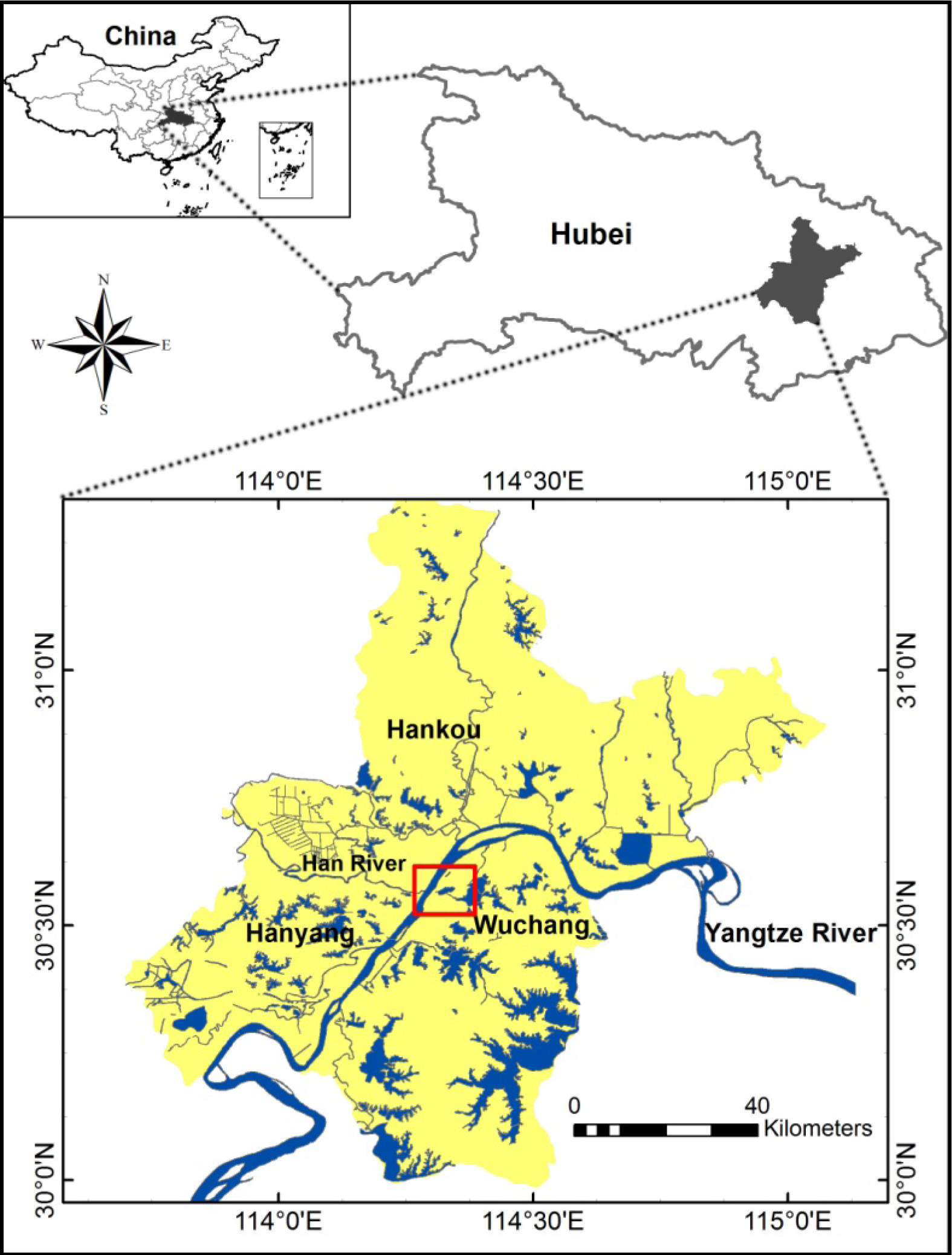
2. Study Area and Data

2.1. Study Area

The study area for this case study is situated in Wuhan City at Hubei Province, Central China (Figure 1). Wuhan City is regarded as a Water City as many rivers and lakes can be found in and around [24,25]. Two large rivers, the Yangtze River and the Han River, flow through the study area and geographically divide the city into three towns: Wuchang, Hankou and Hanyang. The selected site is located in the downtown of Wuchang district, with the longitude ranging from 114°15′N to 114°23′N and the latitude ranging from 30°30′E to 30°37′E. Land use/cover elements are typical of those in urban environments, including rivers, lakes, buildings, roads, woodlands, grasslands, bare land and shadow. In general, rivers and lakes are distributed regularly, grasslands and woodlands are mixed seriously due to the overly fragmented surface of the whole study area, and buildings and roads present different forms. The relatively large coverage, variety of land cover types, combined with fragmented landscape make the site ideal for this study.

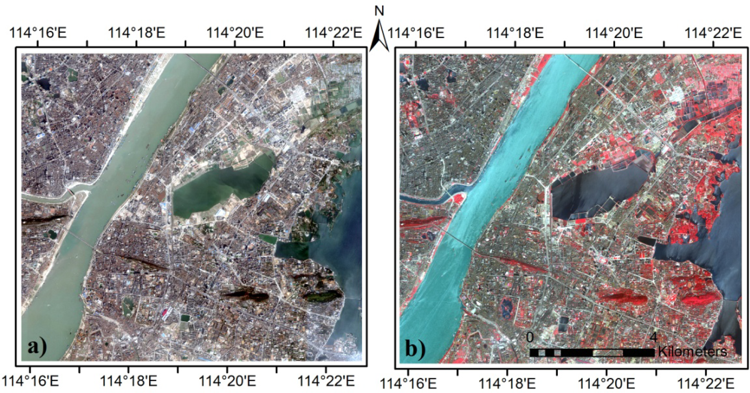
2.2. Data Collection and Processing

The Software GEtScreen ( http://www.godeyes.cn/html/2007/04/09/download_643.html) specialized for Google Earth was used in this study to download four GE images from Google Earth 5.0. These GE images, acquired on 27 March 2003, were originally taken from the QB and have red, green and blue bands with a spatial resolution of 1 m. In order to evaluate the performance of GE images in land use/cover mapping, a real QB image acquired on 19 March 2003, was collected and used for classification accuracy comparison. The QB image has four multi-spectral bands (red, green, blue and near infrared) and one panchromatic band, with a resolution of 2.44 m and 1 m, respectively. The four individual GE images were firstly mosaicked using the ENVI 4.7 software and the mosaicked GE image (Figure 2a) was then registered to the same geographic projection as QB image (Figure 2b) by using 35 ground control points.

To further compare their spectral differences, both QB and GE images were conducted a normalization process by using the formula [26]: $\overline{\mathit{DN}}(i)=\frac{\mathit{DN}(i)}{\mathit{DN}{(i)}_{\text{max}}}$, where $\overline{\mathit{DN}}(i)$ is the normalized digital number ranging from 0 to 1; DN(i) is the original digital number of i band; DN(i)_max is the maximum of original digital number of i band. Based on the normalized images, the coefficient of variation (CV) was calculated and used to describe the spectral consistency and stability for major land cover types in GE and QB images. The comparison of CV for major land cover types between GE and QB images is shown in Figure 3. The GE image generally has a higher CV than QB image, in particular for woodland and shadow classes. This indicates that spectral signatures in one category overlap with other categories in GE image and their pixel homogeneity is significantly lower, resulting in a poor spectral discrimination for land use/cover mapping. An object-based method, which can make full use of the texture, geometry and other characteristics of GE images except for the spectral information, was thus used in this study and described in more detail later.

3. Object-Based Classification Method

Traditional pixel-based classification approach was widely used in land use/cover mapping [27,28]. Yet, with the increase in spatial resolution, single pixel does not capture well the characteristics of targeted objects. The increase in intra-class spectral variability causes a reduction of statistical separability between classes, which is critical to the pixel-based classification methods. Moreover, the pixel-based method is always unable to take advantage of the rich amount of texture characteristics and other detailed spatial information present in the high spatial resolution images. Consequently, classification accuracy is reduced and the classified maps show serious salt-and-pepper effects [29]. For these reasons, an object-based method was used in this study to perform GE classification. The minimum mapping unit of object-based approach is not a pixel but the object composed by groups of adjacent pixels containing specific semantic information. Additionally, except for spectral features, the geometric and texture features of a single object, as well as the topological relationships between different image objects can be frequently utilized in image classification [30]. In this study, the classification process was implemented using the software Defines Developer 8.0 (formerly known as eCognition). It comprises three steps: image segmentation, selection of appropriate features or rules for conducting classification, and classification accuracy assessment and comparison.

3.1. Multi-Scale Image Segmentation

Image segmentation aims to create different image objects that represent meaningful entities (e.g., roofs or vegetation patches) through grouping adjacent pixels with similar characteristics. This is the foundation of subsequent classification because all object features are dependent on the segmented objects [31,32]. It is thus important to develop an appropriate segmentation scheme. In this study, a multi-scale segmentation algorithm embedded in Defines Developer was adopted. It is a bottom-up clustering technique and has been proved to be particularly suitable to high spatial resolution image segmentation [13,33].

Scale factor and heterogeneity criterion are the most important two parameters for image segmentation. The scale factor is indirectly related to the average size of the detected objects while the heterogeneity criterion, determined by mutually exclusive two parameters (i.e., color and shape), controls the clustering decision process [34]. The shape is composed of smoothness and compactness properties. Since land use/cover types differ in spectral and spatial characteristics, if land use/cover types can be segmented at appropriate segmentation scales, the subsequent classification process can be greatly simplified and the mapping accuracy can be significantly improved [23]. Since there is no universally accepted rule to determine the optimal segmentation scale [35], the conventional trial-and-error approach was used here for image segmentation. This method tends to be more reliable and practical in finding the appropriate scale for individual land use/cover types. To do so, we firstly set the different segmentation scales ranging from 20 to 100 with an increment rate of 5. Secondly, the segmentation results were visually analyzed to examine whether the image objects matched the feature boundaries well. By this iteration, the relatively optimal scale for a certain land cover type can be finally determined. As a result, a three-level segmentation scheme was achieved. The first level targeted at larger land use/cover types and the third level optimized for the smaller ones. The appropriate segmentation scales and the parameters associated with heterogeneity criterion of the three-level segmentation scheme were shown in

Table 1. Parameter settings for multi-scale segmentation of GE imagery.

Level	Land Use/Cover Types	Segmentation Scale	Shape	Compactness
1	River, Lake	80	0.2	0.5
2	Bare land, Shadow, Building, Road	50	0.2	0.5
3	Grassland, Woodland	30	0.2	0.5

.

3.2. Feature Selection and Classification Rule

Object features include the spectral, shape, size, texture, and context characteristics. Features usually define the upper and lower limits of a range of measurable characteristics of objects. Image objects within the defined limits are assigned to a specific class, while those outside of the ranges are assigned to other classes [36]. The feature selection is thus to search out the most relevant features for each class so as to help efficiently perform an image classification with a high accuracy [32].

In this study, a total of nine features, including brightness, mean DN, standard deviation of DN, length, ratio of length and width, area, neighborhood relationships between classes, inclusive relationships between classes, and the customized green band ratio (DN of green band/(DN of red band + DN of green band)), were selected by combining the literature review, expert knowledge and visual examination [37,38]. The threshold values of the selected feature were then determined according to the mean and standard deviation of the features [39].

Table 2. Variables and rules used for GE imagery classification.

Level	Parent Class	Child Class	Rule Sets
1	The whole imagery	Land River Lake	1. Brightness and mean DN of spectral bands were used to classify the three classes based on the nearest neighbor classifier. 2. “relborder to river > 0.3” was employed to remove the river objects from the lake objects and “rel_border to river > 0.02” was utilized to remove the lake objects from the river objects. 3. “area < 150,000” was used to correct the misclassified river objects to lake objects. 4. The inclusion relationships between building and river objects were taken to remove the building objects from river objects.
2	Land	Vegetation Shadow (buildings) Others: road Bare land Buildings1	5. The features including brightness, mean DN of each layer and standard deviation were adopted to classify the vegetation, shadow and the remaining class based on the nearest neighbor classifier. 6. “Length/width > 3” was used to classify road objects and “length < 100” was employed to correct misclassifed road objects to building objects. 7. “105 < brightness < 140” and “0.32 < green band ratio < 0.329” were utilized to identify the bareland objects. 8. The remaining objects were classified into building objects.
3	Vegetation Shadow(buildings)	Grassland Woodland Buildings2	9. “Brightness ≥ 55” was employed for grassland objects. 10. “Brightness < 55” was used for woodland objects. 11. “area > 400000” and “brightness > 70” were taken to correct misclassifed shadow objects to building objects.

listed the hierarchical features and rules developed for GE classification in this study. It is worthwhile to note that if only the spectral feature of GE imagery was adopted to identify the specific classes, it can cause some confusion between different classes, such as shadow and woodland, river and lake. When spatial features such as area, neighborhood relationships of objects were included, better classification results could be achieved.

3.3. Classification Accuracy Assessment and Comparison

To evaluate the GE classification performance, one QB image was used in this study and performed the same object-based classification. A complete description on QB image processing and classification has been documented in Hu et al. [40]. The GE-based and QB-based classification accuracies were individually assessed by using a number of independent validation points generated by a random sampling scheme. The accuracy results were then compared to check their difference. This method was widely used in existing studies [27,41,42] as it can minimize the statistical and human bias in the process of validation sample selections [43]. It was implemented in three steps in this study.

The first step was to calculate the total number of validation points based on the following polynomial distribution formula [26]:

$$N=\frac{{\chi }^2(n,1-\frac{1-\alpha }{\kappa })}{4*b^2}$$

(1)

where b presents the expecting accuracy for a specific class, n is the degree freedom of chi-square distribution, α is the confidence level, and κ is the total number of land cover types. In this study, κ was set to 8 as there are 8 land use/cover types, α was set to 85% and b was 5%. Using the above formula, there are totally 570 validation points needed in this study.

The second step aimed to reasonably assign the 570 validation points to individual classes in GE-based and QB-based classification. An average of 50 points was preliminarily distributed to each land use/cover type to ensure that each class, disregarding its area, can gain enough sampling points for accuracy assessment. The remaining points were then proportionally assigned to the related classes by considering their total number of pixels, that is, the larger area the class is, the more sampling points it has. By doing this, it can generate a statistically reasonable number of validation points for individual classes, which were later used to make an accuracy assessment for GE-based and QB-based classification, respectively. Some statistics including overall accuracy, Kappa coefficient, user accuracy and producer accuracy were computed for each thematic map and then compared between them. This procedure was iterated three times to make the assessment objectively and adequately.

Finally, a Z-test between GE-based and QB-based classification accuracy was performed to investigate their differences in significance using the following formula [44]:

$$Z=\frac{\frac{X_1}{N_1}-\frac{X_2}{N_2}}{\sqrt{\rho (1-\rho )(\frac{1}{N_1}+\frac{1}{N_2})}}$$

(2)

where N₁ and N₂ refer to the total number of sampling points, X₁ and X₂ represent the total number of points that was correctly classified, and ρ is calculated by (X₁+X₂)/(N₁+N₂).The derived Z value is subsequently compared against tabulated Z values at the widely used 5% level of significance to indicate its statistical significance of the differences between the compared thematic maps. Thus if |Z| calculated from Equation (2) is ≥ 1.96, there is statistically significant difference between GE and QB classification results.

4. Results and Discussions

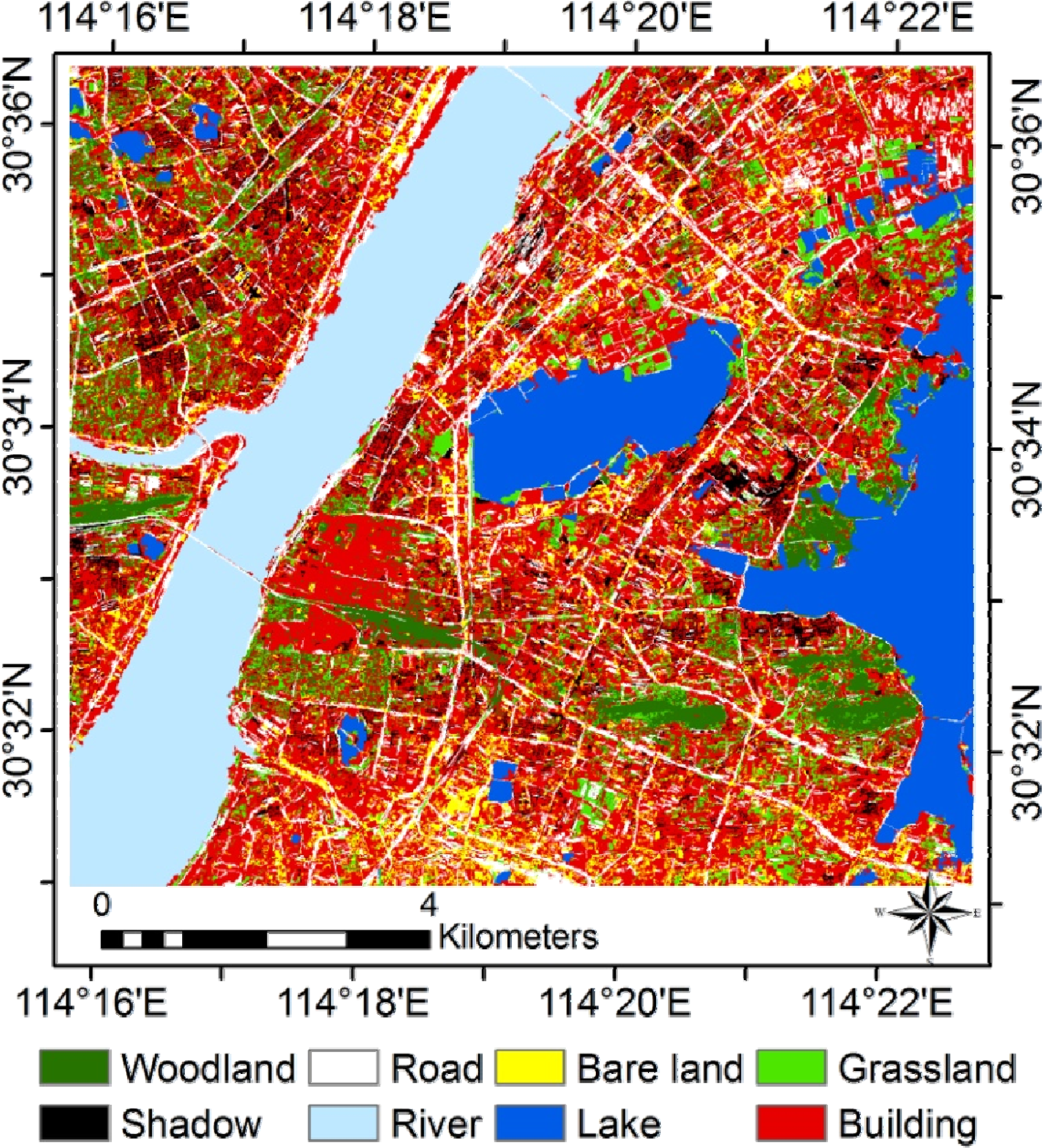
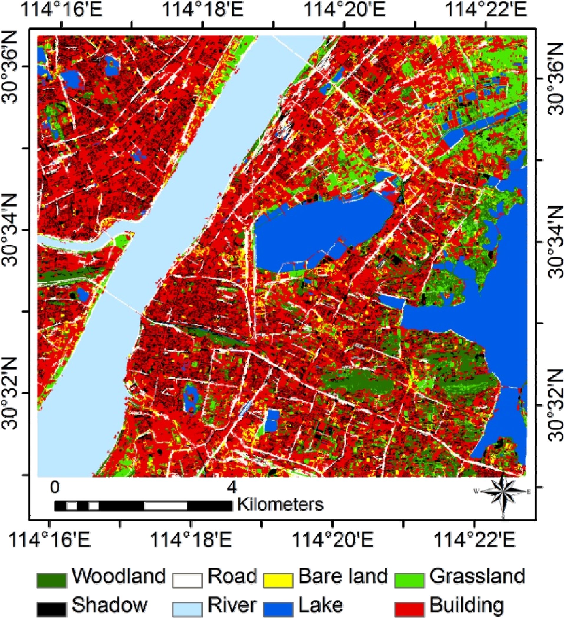
4.1. GE-Based Classification Map

Figure 4 shows the thematic map of land use/cover derived from GE imagery. The statistics of individual land cover types are listed in the

Table 3. The statistics of eight land use/cover types.

	Road	Bare Land	Shadow	Grassland	Woodland	Building	Lake	River
Area (km2)	14.186	7.36	6.183	7.62	5.927	45.064	12.52	15.717
Area proportion (%)	12.38	6.42	5.4	6.65	5.17	39.33	10.93	13.72

. It can be seen that the largest land clover type in this study area is the built-up area with a total area of 45.06 km², accounting for about 39.33% of the totals of the study area. The roads, lakes and rivers share the similar area proportion with a value of 12.38%, 10.93% and 13.72%, respectively. By contrast, other land cover types, including woodland, grassland and shadow, have a relatively lower area proportion, which is less than 7%.

When looking at the spatial distribution of individual classes, it was found that water bodies (including rivers and lakes) in this study area are more convergent in comparison with other classes. Yangtze River flows from the north to the south, dividing the entire study area into two parts, i.e., the east and the west. The two major lakes (Sha Lake and Dong Lake) are obviously distributed in the eastern part due to their large areas. The spatial characteristics of other land use/cover types are more complicated. The woodland is mixed with the grassland, the bare land is fragmented, and the roads are inter-linked and unregularly located everywhere in the study area. In addition, most of the shadow exists between buildings, mainly due to the shelter of the tall buildings.

4.2. Assessment of Classification Accuracy

Figure 5 is the land use/cover map derived from QB imagery. The comparison of classification accuracy between QB and GE imagery was implemented and shown in

Table 4. Comparison of classification accuracy between GE and QB images.

	GE Image		QB Image
	User’s Accuracy (%)	Producer’s Accuracy (%)	User’s Accuracy (%)	Producer’s Accuracy (%)
River	98.72	99.35	99.46	99.25
Lake	88.89	91.18	98.39	93.06
Buildings	79.04	70.28	77.26	75.69
Shadow	80.15	79.46	75.19	88.56
Woodland	58.98	72.02	80.55	79.96
Road	66.78	79.19	77.86	72.76
Bare land	64.21	64.34	62.50	62.64
Grassland	68.26	59.60	76.65	76.64
Overall accuracy(%): QB=81.27, GE=78.07
Kappa statistic: QB=0.78, GE=0.74

. No surprisingly, it can be found that the overall accuracy of GE imagery (78.07% with a Kappa coefficient of 0.74), in general, is slightly lower than that of QB imagery (81.27% with a Kappa coefficient of 0.78).

With respect to individual classes, both GE and QB-based classifications show higher producer’s and user’s accuracy (more than 88.0%) for lakes and rivers, but the lower producer’s and user’s accuracy for bare land (less than 65.0%). The accuracy for buildings and shadow are generally similar in both QB and GE-based classifications (more than 70%), but producer’s accuracy in GE classification is slightly lower than that of QB classification. The classification accuracy of woodland and grassland by using GE imagery are significantly lower than those by using QB imagery, and their average difference is more than 10%. In contrast, the producer’s accuracy of road from GE-based classification is relatively higher than that of QB classification.

Based on the formula 2, |Z| was calculated and equal to 1.34. This suggests that there is no statistical difference between these two classification based on different imagery at the confidence level of 95%, which, in other words, indicates that the classification result of GE imagery is not significantly weaker than that of QB imagery.

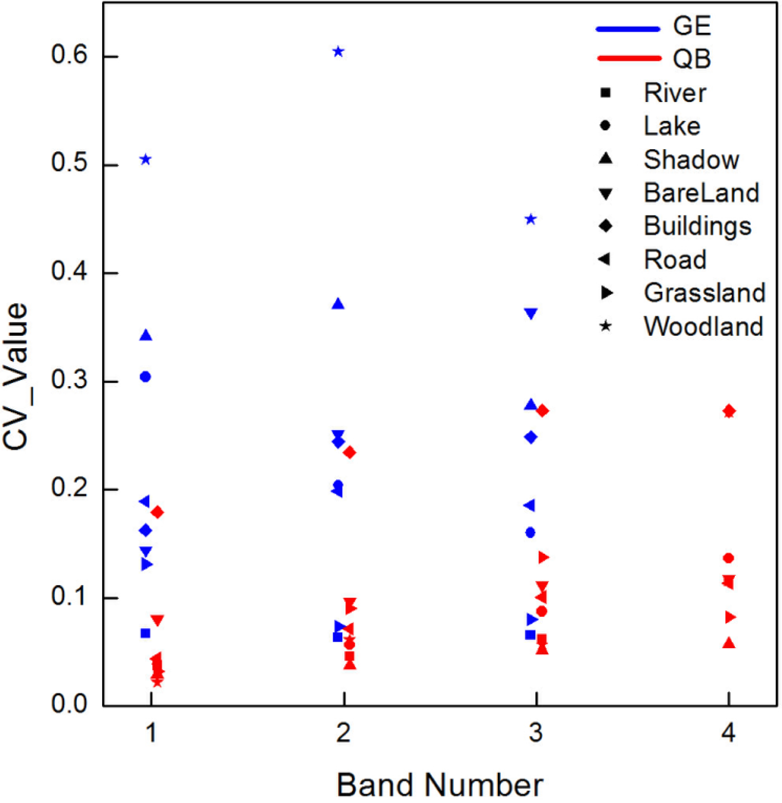
4.3. Potentials Analysis of GE Imagery for Land Use/Cover Mapping

The objective of this study was to perform a land use/cover classification by using GE images as main data sources and to examine their suitability in mapping land use/cover at regional scales. The classification results show that in general, a combination of GE imagery and object-based classification method can achieve an overall accuracy of 78.07%, which is close to the QB classification accuracy (81.27%). Much detailed information for the sub-classes, i.e., roads, buildings and even shadows, which are hardly available in the existing coarse resolution land cover products such as FROM-GLC, GLC2000 and GlobCover, was well recorded in this experiment. This suggests the great potentials of GE imagery in regional land use/cover mapping.

It was found that GE imagery has different discrimination capacity for different land cover types, which is mostly attributed to the characteristics of GE imagery and individual objects. The category of water bodies like rivers and lakes is featured by their relatively better pixel homogeneity and good spectral discrimination. This can be easily captured by GE imagery although it has only three visible bands, resulting in a higher accuracy in these classes than other classes. The GE-based classification for roads has higher producer’s accuracy than that of QB-based classification. This may be explained by the proposal that road classification mainly relies on its shape features, as shown in Table 2, this information can be well derived from GE imagery. Similarly, shadow presents a relatively higher accuracy in comparison with woodland, grassland and bare land as its area characteristics was used for classification (Table 2). This suggests that when using GE imagery for land use/cover mapping, more attention should be given to its spatial characteristics (such as shape, texture and context of objects) in the classification algorithm as these are well described in GE imagery. This conclusion agrees well with the study by Huang et al., which showed that the QB classification based on spatial features (i.e., shape index, length-width ratio) is significantly better than that based on spectral bands [45].

Yet, when comparing with QB imagery, GE imagery has a lower discrimination for grassland and woodland types. This is due to the fact that rather than geometric features, spectral features such as brightness and DN were utilized in identification of grassland and woodland (shown in Table 2). This highlights that the nature of poor spectral information in GE imagery hinders its mapping accuracy to those land cover types, which are classified only by using spectral characteristics. Therefore, the sole spectral-based supervision and unsupervised methods may not be well suited for GE imagery classification [40].

It can be found in Table 4 that both GE and QB-based classifications have the lowest accuracy for bare lands. This is mostly because co-existing of different objects in bare lands results in poor intra-class spectral stability (Figure 3), which makes the spectral signatures overlap with other categories and the spatial characteristics of satellite imagery more heterogenic and complex. This emphasizes that the landscape structure can influence the accuracy of land cover mapping by using satellite data, and the mixed unit problem seems to be a major challenge for land cover mapping efforts because the heterogeneity of the landscape structure is more detailed than the resolution of the satellite sensor [46].

This study also shows that the object-based classification method proved to be an appropriate alternative when using GE imagery for mapping land use/cover. Except for its spectral characteristics, it can make full use of the spatial features of objects, which can, to some degrees, strengthen the advantages of GE imagery for its high spatial resolution and compensate its limitation of poor spectral information. This is consistent with some previous studies, which underlined the specific superiority of object-based methods over traditional pixel-based classifiers for mapping land use/cover [47–49]. Therefore, the spatial features of objects in target need to be utilized as more as possible when performing an object-based classification on GE imagery, in particular when the spectral features cannot identify the targets accurately. In the case that both spectral and spatial characteristics of objects are quite vague in GE imagery, other ancillary data such as DEM, slope and aspect could be taken into consideration and may improve the classification accuracy [50,51]. It is expected that the inclusion of DEM data into the future list could improve the identification capacity between woodland and grassland types, as well as between buildings and shadows, which are significantly confused in this study [42,52].

4.4. Uncertainty Analysis of GE Imagery for Land Use/Cover Mapping

Cropland was not considered as an independent land cover type in this study due to its small area proportion. Instead, land units with green crops were identified as grassland, which may result in a slight overestimation of total grassland area. In addition, we distinguished shadow as an independent type out of the regular human-made impervious surfaces (e.g., building), because of its large area proportion. This could underestimate the area of buildings as most of the shadow area is interrelated and overlaid with building area.

Another factor that contributes to the overall uncertainty is the parameters used in the object-based classification. The proposed segmentation scales and rule-sets were moderately appropriate but may not be the most optimal for this study. This indicates that it is difficult to guarantee the comparisons between the QB and GE imagery performed at their best state, and the potential of GE imagery for land use/cover mapping cannot be assessed completely. Moreover, the trial-and-error approach used for image segmentation in this study is time-consuming and subject to some human influence. A more specific algorithm for image segmentation in future studies would be worthy of consideration for reducing the time of visual interpretation and for determining the relatively “optimal scale” for subsequent analysis.

Possible limitations are also due to the site-specific landscape structure which varies from one place to another and may have some impacts on the classification accuracy. Thus, in the future some more regions and GE images from different satellites or sensors (e.g., IKONOS, SPOT, and RapidEye) need to be tested in a broad scale to make the research findings in this study more robust. Additionally, GE imagery is limited for presenting the dynamic changes in land use/cover as they are inconsistently acquired and have different temporal frequencies [20]. The problem of how to make the best use of the free and high-resolution data for mapping dynamics of land use/cover should be discussed in more detail in the future (e.g., land change monitoring and modeling [53]).

5. Conclusion

The freely accessible GE images were used here as direct data resources (rather than being used as “pictures” for visualization) to perform a classification so as to investigate their potential suitability for mapping complex land use/cover. To do so, the Wuhan city with high heterogeneous landscape was selected for a case study and an object-based classification method was employed to identify the eight targeted land use/cover types. By comparing the GE-based classification result with a reference QB-based classification, it proved that GE imagery possesses some potential for land use/cover mapping as there was no general statistical difference existing between these two classification results. However, due to the unique characteristics of GE imagery (i.e., rich spatial features with low spectral discrimination), the classification accuracy varied greatly according to individual objects: GE imagery has great advantages for mapping land use/cover types with good spatial characteristics in terms of geometric, shape and context (e.g., road and river), but it performs a little worse for mapping land use/cover types that requires high spectral signature (e.g., grassland and woodland). Considering this limitation, other ancillary data is suggested to be included to improve its classification accuracy. To conclude, the object-based method is recommended for image classification when using GE imagery for mapping land use/cover, because it can simultaneously make the best use of spatial characteristics and eliminate the limitations of poor spectral characteristics of GE imagery. Future studies should consider the cross-site comparisons of method application, selection of optimal segmentation scale, and elimination of limitations brought by the inconsistent and multi-temporal data acquisition scheme of GE imagery.

References

1. Colditz, R.R.; Schmidt, M.; Conrad, C.; Hansen, M.C.; Dech, S. Land cover classification with coarse spatial resolution data to derive continuous and discrete maps for complex regions. Remote Sens. Environ 2011, 115, 3264–3275. [Google Scholar]
2. Sleeter, B.M.; Sohl, T.L.; Loveland, T.R.; Auch, R.F.; Acevedo, W.; Drummond, M.A.; Sayler, K.L.; Stehman, S.V. Land-cover change in the conterminous United States from 1973 to 2000. Glob. Environ. Chang 2013, 23, 733–748. [Google Scholar]
3. Wu, W.; Shibasaki, R.; Yang, P.; Zhou, Q.; Tang, H. Remotely sensed estimation of cropland in China: A comparison of the maps derived from four global land cover datasets. Can. J. Remote Sens 2008, 34, 467–479. [Google Scholar]
4. Bargiel, D.; Herrmann, S. Multi-temporal land-cover classification of agricultural areas in two European regions with high resolution spotlight TerraSAR-X data. Remote Sens 2011, 3, 859–877. [Google Scholar]
5. Wang, Y.; Mitchell, B.R.; Nugranad-Marzilli, J.; Bonynge, G.; Zhou, Y.; Shriver, G. Remote sensing of land-cover change and landscape context of the National Parks: A case study of the Northeast temperate network. Remote Sens. Environ 2009, 113, 1453–1461. [Google Scholar]
6. Jiang, H.; Zhao, D.; Cai, Y.; An, S. A method for application of classification tree models to map aquatic vegetation using remotely sensed images from different sensors and dates. Sensors 2012, 12, 12437–12454. [Google Scholar]
7. Zhou, H.; Aizen, E.; Aizen, V. Deriving long term snow cover extent dataset from AVHRR and MODIS data: Central Asia case study. Remote Sens. Environ 2013, 136, 146–162. [Google Scholar]
8. Wijedasa, L.S.; Sloan, S.; Michelakis, D.G.; Clements, G.R. Overcoming limitations with Landsat imagery for mapping of peat swamp forests in Sundaland. Remote Sens 2012, 4, 2595–2618. [Google Scholar]
9. Gong, P.; Wang, J.; Yu, L.; Zhao, Y.; Zhao, Y.; Liang, L.; Niu, Z.; Huang, X.; Fu, H.; Liu, S.; et al. Finer resolution observation and monitoring of global land cover: First mapping results with Landsat TM and ETM+ data. Int. J. Remote Sens 2013, 34, 2607–2654. [Google Scholar]
10. Hansen, M.C.; DeFries, R.S.; Townshend, J.R.; Sohlberg, R. Global land cover classification at 1 km spatial resolution using a classification tree approach. Int. J. Remote Sens 2000, 21, 1331–1364. [Google Scholar]
11. Tchuenté, A.T.K.; Roujean, J.L.; De Jong, S.M. Comparison and relative quality assessment of the GLC2000, GLOBCOVER, MODIS and ECOCLIMAP land cover data sets at the African continental scale. Int. J. Appl. Earth Obs. Geoinf 2011, 13, 207–219. [Google Scholar]
12. Liu, J.; Liu, M.; Deng, X.; Zhuang, D.; Zhang, Z.; Luo, D. The land use and land cover change database and its relative studies in China. J. Geogr. Sci 2002, 12, 275–282. [Google Scholar]
13. Zhou, W.; Troy, A.; Grove, M. Object-based land cover classification and change analysis in the Baltimore metropolitan area using multitemporal high resolution remote sensing data. Sensors 2008, 8, 1613–1636. [Google Scholar]
14. Laliberte, A.S.; Browning, D.M.; Rango, A. A comparison of three feature selection methods for object-based classification of sub-decimeter resolution UltraCam-L imagery. Int. J. Appl. Earth Obs. Geoinf 2012, 15, 70–78. [Google Scholar]
15. Duro, D.C.; Franklin, S.E.; Dubé, M.G. A comparison of pixel-based and object-based image analysis with selected machine learning algorithms for the classification of agricultural landscapes using SPOT-5 HRG imagery. Remote Sens. Environ 2012, 118, 259–272. [Google Scholar]
16. Batista, M.H.; Haertel, V. On the classification of remote sensing high spatial resolution image data. Int. J. Remote Sens 2010, 31, 5533–5548. [Google Scholar]
17. Clark, M.L.; Aide, T.M.; Grau, H.R.; Riner, G. A scalable approach to mapping annual land cover at 250 m using MODIS time series data: A case study in the Dry Chaco Ecoregion of South America. Remote Sens. Environ 2010, 114, 2816–2832. [Google Scholar]
18. Mering, C.; Baro, J.; Upegui, E. Retrieving urban areas on Google Earth images: Application to towns of West Africa. Int. J. Remote Sens 2010, 31, 5867–5877. [Google Scholar]
19. Kaimaris, D.; Georgoula, O.; Patias, P.; Stylianidis, E. Comparative analysis on the archaeological content of imagery from Google Earth. J. Cult. Herit 2011, 12, 263–269. [Google Scholar]
20. Yu, L.; Gong, P. Google Earth as a virtual globe tool for Earth science applications at the global scale: Progress and perspectives. Int. J. Remote Sens 2011, 33, 3966–3986. [Google Scholar]
21. Guo, J.; Liang, L.; Gong, P. Removing shadows from Google Earth images. Int. J. Remote Sens 2010, 31, 1379–1389. [Google Scholar]
22. Potere, D. Horizontal positional accuracy of Google Earth’s high-resolution imagery Archive. Sensors 2008, 8, 7973–7981. [Google Scholar]
23. Drǎguţ, L.; Tiede, D.; Levick, S.R. ESP: A tool to estimate scale parameter for multiresolution image segmentation of remotely sensed data. Int. J. Geogr. Inf. Sci 2010, 24, 859–871. [Google Scholar]
24. Xiao, Y. Spatial-Temporal Land Use Patterns and Master Planning in Wuhan, China. Wuhan University, Wuhan, Hubei, China, 2002. [Google Scholar]
25. Cheng, J.; Masser, I. Urban growth pattern modeling: A case study of Wuhan city, PR China. Landsc. Urban. Plan 2003, 62, 199–217. [Google Scholar]
26. Jensen, J.R. Thematic Map Accuracy Assessment. In Introductory Digital Image Processing: A Remote Sensing Perspective, 3rd ed; Prentice Hall: Upper Saddle River, NJ, USA, 2005; pp. 476–482. [Google Scholar]
27. Shao, Y.; Lunetta, R.S. Comparison of support vector machine, neural network, and CART algorithms for the land-cover classification using limited training data points. ISPRS J. Photogramm. Remote Sens 2012, 70, 78–87. [Google Scholar]
28. Aitkenhead, M.J.; Aalders, I.H. Automating land cover mapping of Scotland using expert system and knowledge integration methods. Remote Sens. Environ 2011, 115, 1285–1295. [Google Scholar]
29. Yu, Q.; Gong, P.; Clinton, N.; Biging, G.; Kelly, M.; Schirokauer, D. Object-based detailed vegetation classification with airborne high spatial resolution remote sensing imagery. Photogramm. Eng. Remote Sens 2006, 72, 799–811. [Google Scholar]
30. Lisita, A.; Sano, E.E.; Durieux, L. Identifying potential areas of Cannabis sativa plantations using object-based image analysis of SPOT-5 satellite data. Int. J. Remote Sens 2013, 34, 5409–5428. [Google Scholar]
31. Lu, D.; Weng, Q. A survey of image classification methods and techniques for improving classification performance. Int. J. Remote Sens 2007, 28, 823–870. [Google Scholar]
32. Blaschke, T. Object based image analysis for remote sensing. ISPRS J. Photogramm. Remote Sens 2010, 65, 2–16. [Google Scholar]
33. Dribault, Y.; Chokmani, K.; Bernier, M. Monitoring seasonal hydrological dynamics of minerotrophic peatlands using multi-date GeoEye-1 very high resolution imagery and object-based classification. Remote Sens 2012, 4, 1887–1912. [Google Scholar]
34. Mathieu, R.; Aryal, J.; Chong, A. Object-based classification of Ikonos imagery for mapping large-scale vegetation communities in urban areas. Sensors 2007, 7, 2860–2880. [Google Scholar]
35. Myint, S.W.; Gober, P.; Brazel, A.; Grossman-Clarke, S.; Weng, Q. Per-pixel vs. object-based classification of urban land cover extraction using high spatial resolution imagery. Remote Sens. Environ 2011, 115, 1145–1161. [Google Scholar]
36. Manandhar, R.; Odeh, I.; Ancev, T. Improving the accuracy of land use and land cover classification of landsat data using post-classification enhancement. Remote Sens 2009, 1, 330–344. [Google Scholar]
37. Zhou, W.; Troy, A. An object-oriented approach for analysing and characterizing urban landscape at the parcel level. Int. J. Remote Sens 2008, 29, 3119–3135. [Google Scholar]
38. Duro, D.C.; Franklin, S.E.; Dubé, M.G. A comparison of pixel-based and object-based image analysis with selected machine learning algorithms for the classification of agricultural landscapes using SPOT-5 HRG imagery. Remote Sens. Environ 2012, 118, 259–272. [Google Scholar]
39. Benz, U.C.; Hofmann, P.; Willhauck, G.; Lingenfelder, I.; Heynen, M. Multi-resolution, object-oriented fuzzy analysis of remote sensing data for GIS-ready information. ISPRS J. Photogramm. Remote Sens 2004, 58, 239–258. [Google Scholar]
40. Hu, Q.; Zhang, J.; Xu, B.; Li, Z. A comparison of Google Earth imagery and the homologous Quick Bird imagery being used in land-use classification. J. Huazhong Norm. Univ 2013, 52, 287–291. [Google Scholar]
41. Gao, Y.; Mas, J.F.; Navarrete, A. The improvement of an object-oriented classification using multi-temporal MODIS EVI satellite data. Int. J. Digit. Earth 2009, 2, 219–236. [Google Scholar]
42. Zhou, W.; Huang, G.; Troy, A.; Cadenasso, M.L. Object-based land cover classification of shaded areas in high spatial resolution imagery of urban areas: A comparison study. Remote Sens. Environ 2009, 113, 1769–1777. [Google Scholar]
43. Ghosh, A.; Joshi, P.K. A comparison of selected classification algorithms for mapping bamboo patches in lower Gangetic plains using very high resolution WorldView 2 imagery. Int. J. Appl. Earth Obs. Geoinf 2014, 26, 298–311. [Google Scholar]
44. Foody, G.M. Thematic map comparison: Evaluating the statistical significance of differences in classification accuracy. Photogramm. Eng. Remote Sens 2004, 5, 627–633. [Google Scholar]
45. Huang, X.; Zhang, L.; Li, P. Classification and extraction of spatial features in urban areas using high-resolution multispectral imagery. IEEE Geosci. Remote Sens.Lett 2007, 4, 260–264. [Google Scholar]
46. Smith, A. Image segmentation scale parameter optimization and land cover classification using the Random Forest algorithm. J. Spat. Sci 2010, 55, 69–79. [Google Scholar]
47. Castillejo-González, I.L.; López-Granados, F.; García-Ferrer, A.; Peña-Barragán, J.M.; Jurado-Expósito, M.; de la Orden, M.S.; González-Audicana, M. Object- and pixel-based analysis for mapping crops and their agro-environmental associated measures using QuickBird imagery. Comput. Electron. Agric 2009, 68, 207–215. [Google Scholar]
48. Petropoulos, G.P.; Kalaitzidis, C.; Prasad Vadrevu, K. Support vector machines and object-based classification for obtaining land-use/cover cartography from Hyperion hyperspectral imagery. Comput. Geosci 2012, 41, 99–107. [Google Scholar]
49. Elatawneh, A.; Kalaitzidis, C.; Petropoulos, G.P.; Schneider, T. Evaluation of diverse classification approaches for land use/cover mapping in a Mediterranean region utilizing Hyperion data. Int. J. Digit. Earth 2012. [Google Scholar] [CrossRef]
50. Anders, N.S.; Seijmonsbergen, A.C.; Bouten, W. Segmentation optimization and stratified object-based analysis for semi-automated geomorphological mapping. Remote Sens. Environ 2011, 115, 2976–2985. [Google Scholar]
51. Salehi, B.; Zhang, Y.; Zhong, M.; Dey, V. Object-based classification of urban areas using VHR imagery and height points ancillary data. Remote Sens 2012, 4, 2256–2276. [Google Scholar]
52. Haala, N.; Brenner, C. Extraction of buildings and trees in urban environments. ISPRS J. Photogramm. Remote Sens 1999, 54, 130–137. [Google Scholar]
53. Yu, Q.; Wu, W.; Yang, P.; Li, Z.; Xiong, W.; Tang, H. Proposing an interdisciplinary and cross-scale framework for global change and food security researches. Agric. Ecosyst. Environ 2012, 156, 57–71. [Google Scholar]
Figure 1. Location of the study area in Hubei, China.
Remotesensing 05 06026f1
Figure 2. Satellite images used in this study (a): Google Earth (GE) image, (b): QuickBird (QB) image.
Remotesensing 05 06026f2
Figure 3. Comparison of the coefficient of variation (CV) between GE and QB image for major land cover types.
Remotesensing 05 06026f3
Figure 4. Land use/cover map derived from GE imagery.
Remotesensing 05 06026f4
Figure 5. Land use/cover map derived from QB imagery.
Remotesensing 05 06026f5