Multi-Decadal Mangrove Forest Change Detection and Prediction in Honduras, Central America, with Landsat Imagery and a Markov Chain Model


Abstract
:1. Introduction
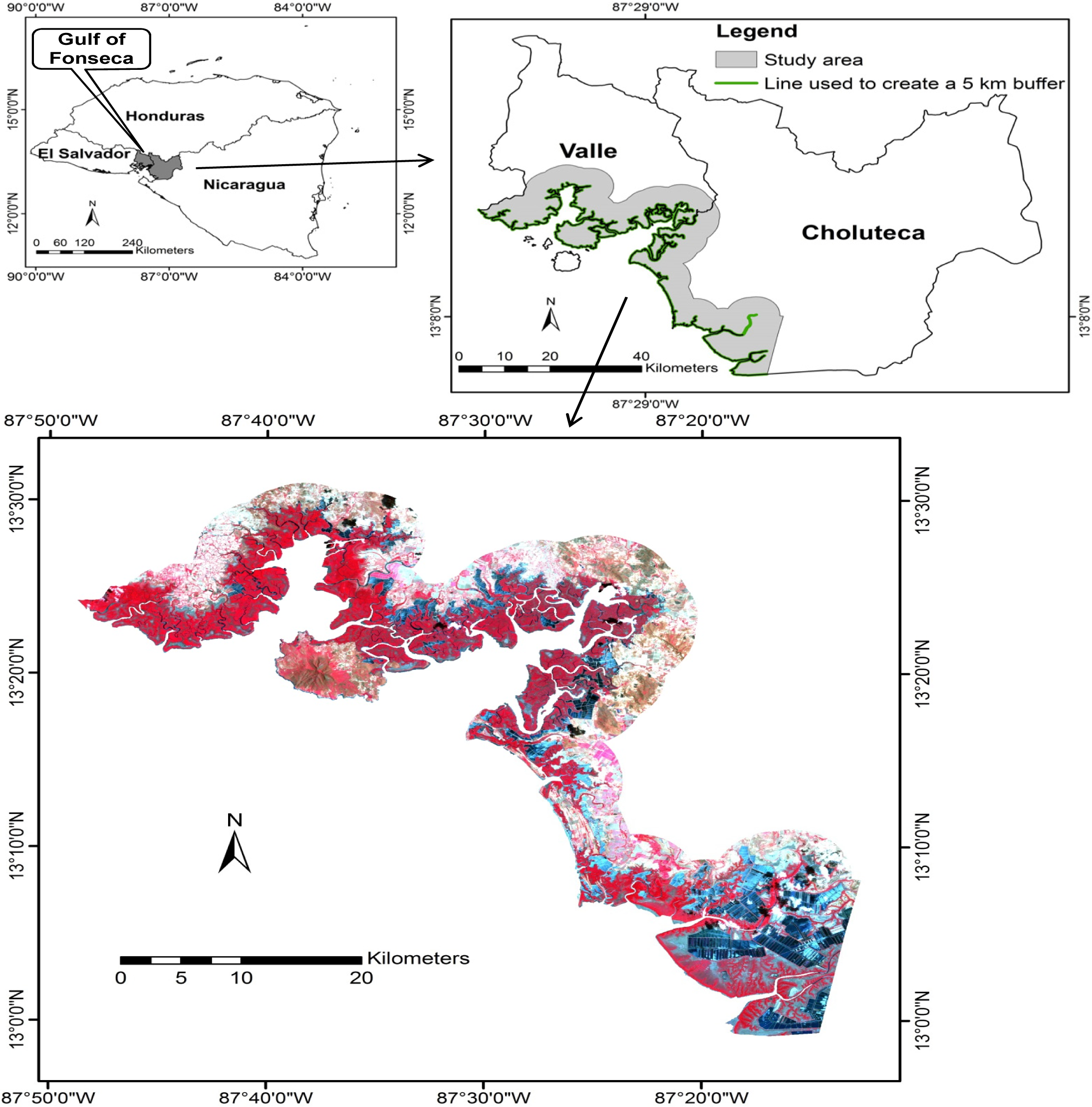
2. Study Area
3. Data Collection
4. Methodology
4.1. Data Pre-Processing
4.2. Image Classification and Change Detection
4.2.1. Non-Vegetated Area Masking
4.2.2. Spectral Band Selection
4.2.3. Mangrove Extraction and Change Detection
4.3. Mangrove Change Projection
- Pearson’s Chi-square χ2 to test the hypothesis of data independence using:
- Goodness-of-fit test to test the suitability of the Markovian hypothesis by examining the observed and transition matrices during 1996–2013:
5. Results and Discussion
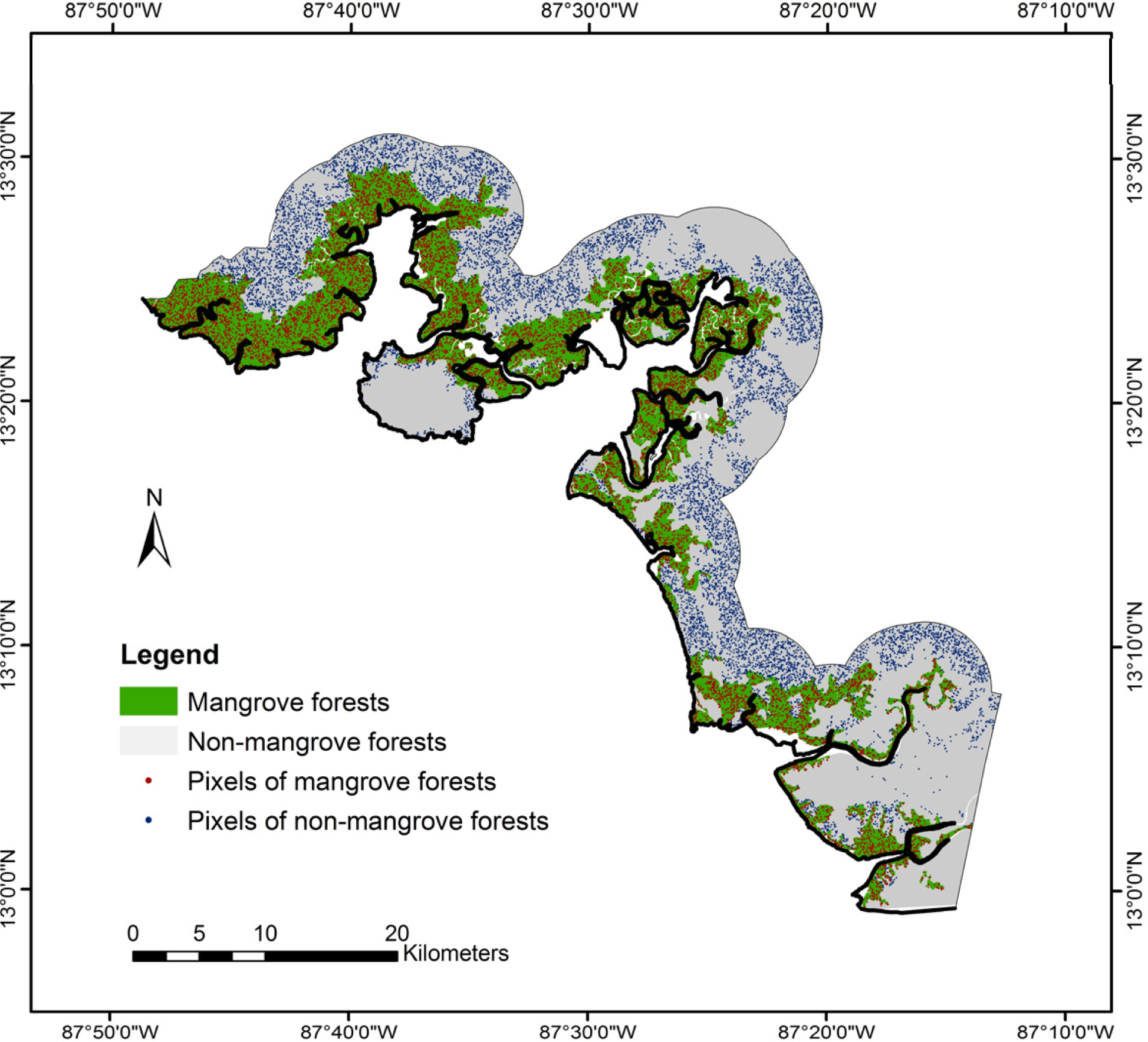
5.1. Spatiotemporal Distribution of Mangrove Forests and Accuracy Assessment Results
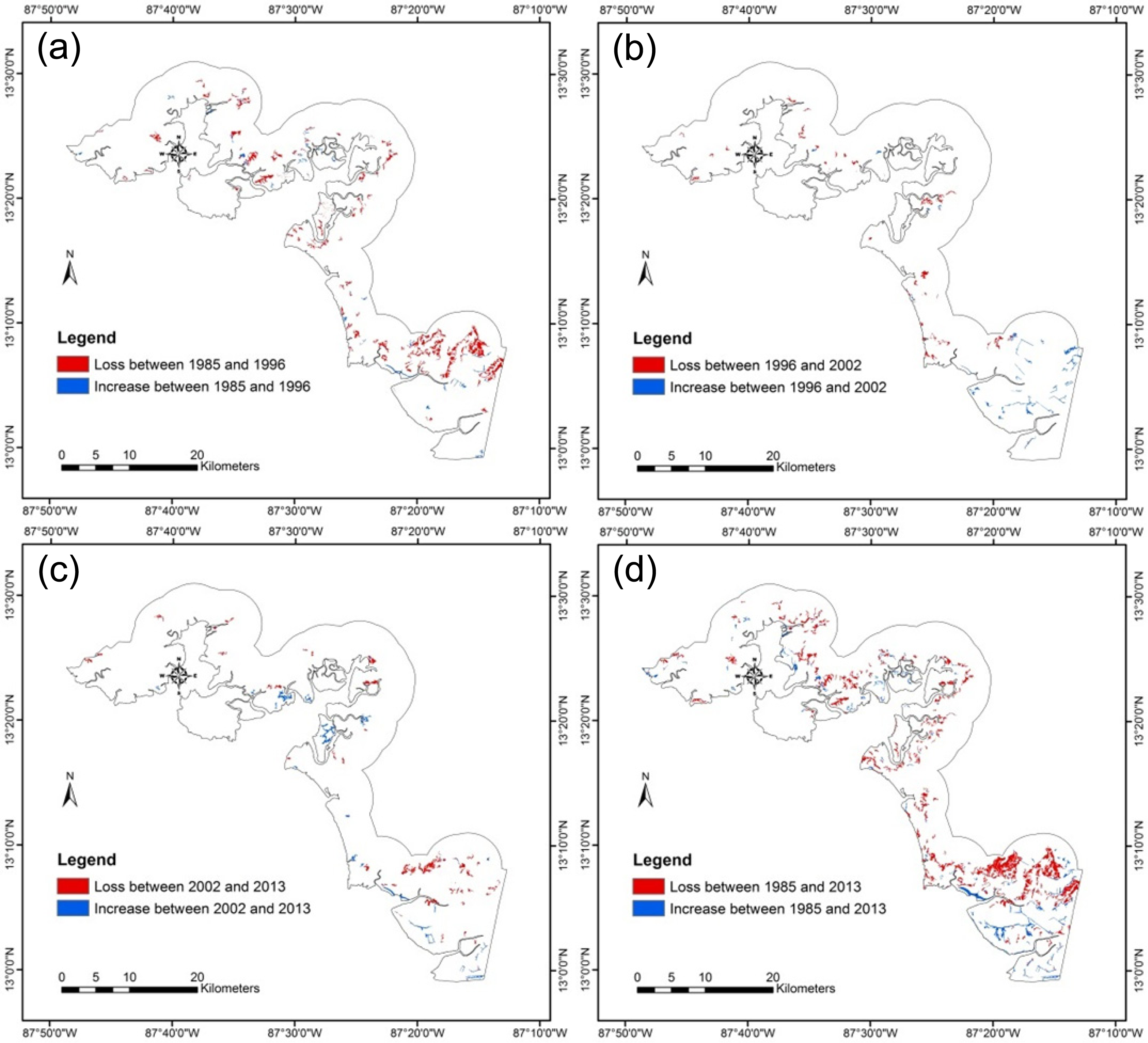
5.2. Mangrove Change Detection
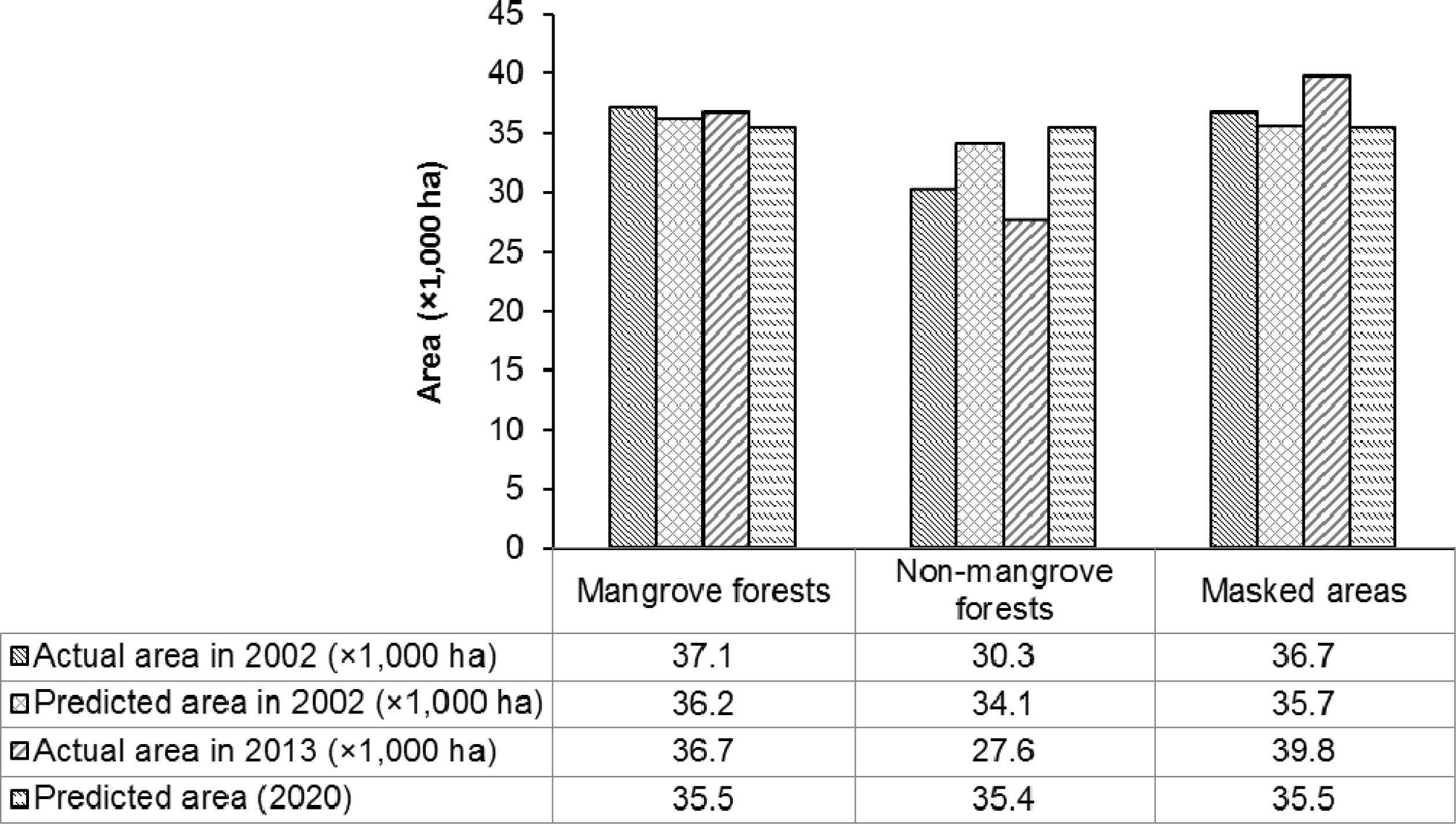
5.3. Mangrove Change Projection
6. Conclusions
Acknowledgments
Conflicts of Interest
References
- Brown, C.; Corcoran, E.; Herkenrath, P.; Thonell, J. Marine and Coastal Ecosystems and Human Well-Being: Synthesis; United Nations Environment Programme, Division of Early Warning Assessment: Nairobi, Kenya, 2006. [Google Scholar]
- Giri, C.; Ochieng, E.; Tieszen, L.L.; Zhu, Z.; Singh, A.; Loveland, T.; Masek, J.; Duke, N. Status and distribution of mangrove forests of the world using earth observation satellite data. Glob. Ecol. Biogeogr 2011, 20, 154–159. [Google Scholar]
- Costanza, R. Visions, values, valuation, and the need for an ecological economics. Bioscience 2001, 51, 459–468. [Google Scholar]
- Nagelkerken, I.; Blaber, S.J.M.; Bouillon, S.; Green, P.; Haywood, M.; Kirton, L.G.; Meynecke, J.O.; Pawlik, J.; Penrose, H.M.; Sasekumar, A.; et al. The habitat function of mangroves for terrestrial and marine fauna: A review. Aquat. Bot 2008, 89, 155–185. [Google Scholar]
- Duke, N.C.; Meynecke, J.O.; Dittmann, S.; Ellison, A.M.; Anger, K.; Berger, U.; Cannicci, S.; Diele, K.; Ewel, K.C.; Field, C.D.; et al. A world without mangroves? Science 2007, 317, 41–42. [Google Scholar]
- Jennerjahn, T.; Ittekkot, V. Relevance of mangroves for the production and deposition of organic matter along tropical continental margins. Naturwissenschaften 2002, 89, 23–30. [Google Scholar]
- Dittmar, T.; Hertkorn, N.; Kattner, G.; Lara, R.J. Mangroves, a major source of dissolved organic carbon to the oceans. Glob. Biogeochem. Cy. 2006, 20. [Google Scholar] [CrossRef]
- Valiela, I.; Bowen, J.L.; York, J.K. Mangrove forests: One of the world’s threatened major tropical environments. BioScience 2001, 51, 807–815. [Google Scholar]
- Giri, C.; Zhu, Z.; Tieszen, L.L.; Singh, A.; Gillette, S.; Kelmelis, J.A. Mangrove forest distributions and dynamics (1975–2005) of the tsunami-affected region of Asia†. J. Biogeogr 2008, 35, 519–528. [Google Scholar]
- FAO. The World’s Mangroves 1980–2005; Food and Agriculture Organization of the United Nations: Rome, Italy, 2007. [Google Scholar]
- Alongi, D.M. Present state and future of the world’s mangrove forests. Environ. Conserv 2002, 29, 331–349. [Google Scholar]
- Tobey, J.; Clay, J.; Vergne, P. Maintaining a Balance: The Economic, Environmental and Social Impacts of Shrimp Farming in Latin America; Coastal Resources Center, University of Rhode Island: Narragansett, RI, USA, 1998. [Google Scholar]
- Stanley, D.L. The economic impact of mariculture on a small regional economy. World Development 2003, 31, 191–210. [Google Scholar]
- FAO. Global Production Statistics 1950–2005; Food and Agriculture Organization of the United Nations: Rome, Italy, 2005. [Google Scholar]
- Stonich, S.C.; Bort, J.R.; Ovares, L.L. Globalization of shrimp mariculture: The impact on social justice and environmental quality in central America. Soc. Nat. Resourc 1997, 10, 161–179. [Google Scholar]
- Paez-Osuna, F. The environmental impact of shrimp aquaculture: A global perspective. Environ. Pollut 2001, 112, 229–231. [Google Scholar]
- Paez-Osuna, F. The environmental impact of shrimp aquaculture: Causes, effects, and mitigating alternatives. Environ. Manag 2001, 28, 131–140. [Google Scholar]
- Bolstad, P.; Lillesand, T.M. Rapid maximum likelihood classification. Photogram. Eng. Remote Sens 1991, 57, 67–74. [Google Scholar]
- Boser, B.E.; Guyon, I.; Vapnik, V. Annual Workshop on Computational Learning Theory. In A Training Algorithm for Optimal Margin Classiers, 5th ed.; ACM Press: New York, NY, USA, 1992. [Google Scholar]
- Benediktsson, J.A.; Swain, P.H.; Ersoy, O.K. Neural Network Approaches vs. Statistical Methods in Classification of Multisource Remote Sensing Data. Proceedings of IEEE International Geoscience and Remote Sensing Symposium (IGARSS’89) & 12th International Canadian Symposium on Remote Sensing, Vancouver, BC, Canada, 10–14 July 1989; pp. 489–492.
- Karkee, M.; Steward, B.L.; Tang, L.; Aziz, S.A. Quantifying sub-pixel signature of paddy rice field using an artificial neural network. Comput. Electron. Agric 2009, 65, 65–76. [Google Scholar]
- Moody, A.; Gopal, S.; Strahler, A.H. Artificial neural network response to mixed pixels in coarse-resolution satellite data. Remote Sens. Environ 1996, 58, 329–343. [Google Scholar]
- Otsu, N. A threshold selection method from gray-level histograms. IEEE Trans. Syst. Man Cybern 1979, 9, 62–66. [Google Scholar]
- Lambin, E.F. Modelling Deforestation Processes: A Review; Office for Official Publications of the European Community: Brussels, Belgium, 1994. [Google Scholar]
- Glenn, D.C.; Lewin, R.K.; Peet, T.T.V. Plant Succession: Theory and Prediction; Chapman & Hall: London, UK, 1992. [Google Scholar]
- Dorigo, M.; Stützle, T. The Ant Colony Optimization Metaheuristic: Algorithms, Applications, and Advances. In Handbook of Metaheuristics; Glover, F., Kochenberger, G., Eds.; Springer: New York, NY, USA, 2003; Volume 57, pp. 250–285. [Google Scholar]
- Von Neumann, J.; Burks, A.W. Theory of Self-Reproducing Automata; University of Illinois Press: Champaign, IL, USA, 1966. [Google Scholar]
- Araya, Y.H.; Cabral, P. Analysis and modeling of urban land cover change in Setúbal and Sesimbra, Portugal. Remote Sens 2010, 2, 1549–1563. [Google Scholar]
- Coppedge, B.; Engle, D.; Fuhlendorf, S. Markov models of land cover dynamics in a southern Great Plains grassland region. Landsc. Ecol 2007, 22, 1383–1393. [Google Scholar]
- Yang, X.; Zheng, X.-Q.; Lv, L.N. A spatiotemporal model of land use change based on ant colony optimization, Markov chain and cellular automata. Ecol. Model 2012, 233, 11–19. [Google Scholar]
- Petit, C.; Scudder, T.; Lambin, E. Quantifying processes of land-cover change by remote sensing: Resettlement and rapid land-cover changes in south-eastern Zambia. Int. J. Remote Sens 2001, 22, 3435–3456. [Google Scholar]
- Rajitha, K.; Mukherjee, C.K.; Vinu Chandran, R.; Prakash Mohan, M.M. Land-cover change dynamics and coastal aquaculture development: A case study in the East Godavari delta, Andhra Pradesh, India using multi-temporal satellite data. Int. J. Remote Sens 2010, 31, 4423–4442. [Google Scholar]
- López, E.; Bocco, G.; Mendoza, M.; Duhau, E. Predicting land-cover and land-use change in the urban fringe: A case in Morelia city, Mexico. Landsc. Urban Plan 2001, 55, 271–285. [Google Scholar]
- Mitsova, D.; Shuster, W.; Wang, X. A cellular automata model of land cover change to integrate urban growth with open space conservation. Landsc. Urban Plan 2011, 99, 141–153. [Google Scholar]
- Silva, E.A.; Ahern, J.; Wileden, J. Strategies for landscape ecology: An application using cellular automata models. Prog. Plan 2008, 70, 133–177. [Google Scholar]
- Han, J.; Hayashi, Y.; Cao, X.; Imura, H. Application of an integrated system dynamics and cellular automata model for urban growth assessment: A case study of Shanghai, China. Landsc. Urban Plan 2009, 91, 133–141. [Google Scholar]
- Adhikari, S.; Southworth, J. Simulating forest cover changes of Bannerghatta National Park based on a CA-markov model: A remote sensing approach. Remote Sens 2012, 4, 3215–3243. [Google Scholar]
- Lepš, J. Mathematical modelling of ecological succesion—A review. Folia Geobot. Phytotax 1988, 23, 79–94. [Google Scholar]
- Du, Y.; Wen, W.; Cao, F.; Ji, M. A case-based reasoning approach for land use change prediction. Expert Syst. Appl 2010, 37, 5745–5750. [Google Scholar]
- Arsanjani, J.J.; Kainz, W.; Mousivand, A.J. Tracking dynamic land-use change using spatially explicit Markov Chain based on cellular automata: The case of Tehran. Int. J. Image Data Fusion 2011, 2, 329–345. [Google Scholar]
- Dorigo, M.; Maniezzo, V.; Colorni, A. Ant system: Optimization by a colony of cooperating agents. IEEE Trans. Syst. Man Cybern. Part B Cybern 1996, 26, 29–41. [Google Scholar]
- Wagner, D.F. Cellular automata and geographic information systems. Environ. Plan. B Plan. Design 1997, 24, 219–234. [Google Scholar]
- Shafizadeh Moghadam, H.; Helbich, M. Spatiotemporal urbanization processes in the megacity of Mumbai, India: A Markov chains-cellular automata urban growth model. Appl. Geogr 2013, 40, 140–149. [Google Scholar]
- Stonich, S.C. Struggling with Honduran poverty: The environmental consequences of natural resource-based development and rural transformations. World Dev 1992, 20, 385–399. [Google Scholar]
- Southworth, J.; Munroe, D.; Nagendra, H. Land cover change and landscape fragmentation—Comparing the utility of continuous and discrete analyses for a western Honduras region. Agric. Ecosyst. Environ 2004, 101, 185–205. [Google Scholar]
- Stonich, S.C. The promotion of non-traditional agricultural exports in Honduras: Issues of equity, environment and natural resource management. Dev. Change 1991, 22, 725–755. [Google Scholar]
- Richards, J.A.; Jia, X. Remote Sensing Digital Image Analysis: An Introduction, 4th ed.; Springer-Verlag: Berlin, Germany, 2006; p. 439. [Google Scholar]
- Woolley, J.T. Reflectance and transmittance of light by leaves. Plant Physiol 1971, 47, 656–662. [Google Scholar]
- Gausman, H.W. Leaf reflectance of near-infrared. Photogram. Eng 1974, 40, 183–191. [Google Scholar]
- Bhattacharyya, A. On a measure of divergence between two statistical populations defined by their probability distributions. Bull. Calcutta Math. Soc 1943, 35, 99–109. [Google Scholar]
- Lim, J.S. Two-Dimensional Signal and Image Processing; Prentice Hall: Upper Saddle River, NJ, USA, 1990. [Google Scholar]
- FAO. State of World Aquaculture; Food and Agriculture Organization of the United Nations: Rome, Italy, 2006. [Google Scholar]
- FAO. The State of World Fisheries and Aquaculture; FAO Fisheries and Aquaculture Department, Food and Agriculture Organization of the United Nations: Rome, Italy, 2007. [Google Scholar]
- Benessaiah, K. Mangroves, Shrimp Aquaculture and Coastal Livelihoods in the Estero Real, Gulf of Fonseca, Nicaragua; McGill University: Montreal, QC, Canada, 2008. [Google Scholar]
- FAO. Regional Review on Aquaculture Development in Latin America and the Caribbean; Food and Agriculture Organization of the United Nations: Rome, Italy, 2006. [Google Scholar]
- Cahoon, D.R.; Hensel, P. Hurricane Mitch: A Regional Perspective on Mangrove Damage, Recovery and Sustainability; USGS: New York, NY, USA, 2002. [Google Scholar]
- Polidoro, B.A.; Carpenter, K.E.; Collins, L.; Duke, N.C.; Ellison, A.M.; Ellison, J.C.; Farnsworth, E.J.; Fernando, E.S.; Kathiresan, K.; Koedam, N.E.; et al. The loss of species: Mangrove extinction risk and geographic areas of global concern. PLoS One 2010, 5. [Google Scholar] [CrossRef]
- Ellison, A.M. Managing mangroves with benthic biodiversity in mind: Moving beyond roving banditry. J. Sea Res 2008, 59, 2–15. [Google Scholar]
- Gilman, E.L.; Ellison, J.; Duke, N.C.; Field, C. Threats to mangroves from climate change and adaptation options: A review. Aquat. Bot 2008, 89, 237–250. [Google Scholar]
- UN. World Population Prospects: The 2012 Revision; United Nations: New York, NY, USA, 2012. [Google Scholar]
- IDB. Integrated Ecosystem Management of the Gulf of Fonseca; Inter-American Development Bank (IDB): Washington, DC, USA, 2007. [Google Scholar]
- Benítez, M.; Machado, M.; Erazo, M.; Aguilar, J.; Campos, A.; Durón, G.; Aburto, C.; Chanchan, R.; Gammage, S. A Platform for Action for the Sustainable Management of Mangroves in the Gulf of Fonseca; International Center for Research on Women: Washington, DC, USA, 2000. [Google Scholar]


| Band (Landsat TM, ETM+) | Band (Landsat OLI) | Band Name | Mangrove Forests vs. non-Mangrove Forests |
|---|---|---|---|
| 1 | 2 | Blue | 0.85 |
| 2 | 3 | Green | 0.98 |
| 3 | 4 | Red | 1.11 |
| 4 | 5 | NIR | 0.33 |
| 5 | 6 | SWIR1 | 1.26 |
| 7 | 7 | SWIR2 | 1.20 |
| Ground Reference Data (pixels) | Classification Results (pixels) | Total | |
|---|---|---|---|
| Mangrove Forests | Non-Mangrove Forests | ||
| Mangrove forests | 9,425 | 575 | 10,000 |
| Non-mangrove forests | 1,213 | 8,787 | 10,000 |
| Total | 10,638 | 9,362 | 20,000 |
| Producer accuracy (%) | 94.3 | 87.9 | |
| User accuracy (%) | 88.6 | 93.9 | |
| Overall accuracy (%) | 91.1 | ||
| Kappa coefficient | 0.82 | ||
| Period | Loss | Increase | ||
|---|---|---|---|---|
| ha | % | ha | % | |
| 1985–1996 | 2,892.3 | 7.3 | 555.3 | 1.4 |
| 1996–2002 | 638.6 | 1.7 | 608.7 | 1.6 |
| 2002–2013 | 1,053.1 | 2.8 | 771.6 | 2.1 |
| 1985–2013 | 4,694.1 | 11.9 | 1,553.2 | 3.9 |
| 1996–2002 | Mangrove Forests | Non-Mangrove Forests | Masked Areas |
|---|---|---|---|
| Mangrove forests | 0.532 | 0.179 | 0.288 |
| Non-mangrove forests | 0.124 | 0.375 | 0.501 |
| Masked areas | 0.236 | 0.201 | 0.563 |
| 1996–2013 | |||
| Mangrove forests | 0.305 | 0.234 | 0.460 |
| Non-mangrove forests | 0.290 | 0.237 | 0.473 |
| Masked areas | 0.297 | 0.236 | 0.468 |
© 2013 by the authors; licensee MDPI, Basel, Switzerland This article is an open access article distributed under the terms and conditions of the Creative Commons Attribution license ( http://creativecommons.org/licenses/by/3.0/).
Share and Cite
Chen, C.-F.; Son, N.-T.; Chang, N.-B.; Chen, C.-R.; Chang, L.-Y.; Valdez, M.; Centeno, G.; Thompson, C.A.; Aceituno, J.L. Multi-Decadal Mangrove Forest Change Detection and Prediction in Honduras, Central America, with Landsat Imagery and a Markov Chain Model. Remote Sens. 2013, 5, 6408-6426. https://doi.org/10.3390/rs5126408
Chen C-F, Son N-T, Chang N-B, Chen C-R, Chang L-Y, Valdez M, Centeno G, Thompson CA, Aceituno JL. Multi-Decadal Mangrove Forest Change Detection and Prediction in Honduras, Central America, with Landsat Imagery and a Markov Chain Model. Remote Sensing. 2013; 5(12):6408-6426. https://doi.org/10.3390/rs5126408
Chicago/Turabian StyleChen, Chi-Farn, Nguyen-Thanh Son, Ni-Bin Chang, Cheng-Ru Chen, Li-Yu Chang, Miguel Valdez, Gustavo Centeno, Carlos Alberto Thompson, and Jorge Luis Aceituno. 2013. "Multi-Decadal Mangrove Forest Change Detection and Prediction in Honduras, Central America, with Landsat Imagery and a Markov Chain Model" Remote Sensing 5, no. 12: 6408-6426. https://doi.org/10.3390/rs5126408