1. Introduction
The notion of a composite satellite image, created from multiple images acquired on multiple dates, is widely used. Holben [
1] introduced the method of using a composite defined by the maximum value of the Normalized Difference Vegetation Index (NDVI) for use with the NOAA AVHRR instrument in order to reduce a range of problems, including “cloud contamination, atmospheric attenuation, surface directional reflectance, and view and illumination geometry” [
1], in the study of vegetation dynamics. Since AVHRR acquires multiple daily imagery, this could be used to produce composites for a seven day period. The technique has also been applied with the Moderate Resolution Imaging Spectroradiometer (MODIS) instrument, in combination with other constraints to help exclude other undesirable artifacts from extreme view angles, cloud contamination, and other sources, producing 16 day vegetation index composites [
2]. Roy
et al. [
3] have used a similar approach to that used for MODIS vegetation indices, applied to Landsat-7 ETM+ imagery, to produce weekly, monthly, seasonal and annual composite images, not only of NDVI itself, but using the selected date (per pixel) to produce composites of the corresponding at-sensor reflectance. In other work with the MODIS sensor, 8 day composites of surface reflectance are created using an algorithm which scores each date, per pixel, to select for dates which minimize sensor and sun zenith angles, cloud and shadow contamination, and aerosol load [
4]. The sun and satellite positions are particularly relevant for the MODIS instrument because it makes two overpasses per day, and has a very wide swath, meaning that both these angles can be quite large. The MODIS instrument also lends itself to another approach to creating a multi-temporal reflectance composite, presented as the MODIS MCD43B4 product [
5]. In this method, a value for surface reflectance is computed from a model of the bi-directional reflectance distribution function (BRDF), which estimates reflectance as a function of sun and satellite angular geometry, and must be parameterized on a per-pixel basis. This is possible because of the high revisit rate of MODIS, allowing parameterization on a 16 day window, with minimal risk of on-ground change invalidating the parameterization, something which is not appropriate for the Landsat TM/ETM+ family, with their much longer revisit interval.
The benefits of producing these kinds of composites are clear. The result is generally a regular time series with minimal missing data or contamination from various sources of noise. The presence of contamination, and the highly variable amount of missing data in different parts of the time series, can present notable difficulties in analysis of long term behavior. Kovalskyy and Roy [
6] provide a world-wide statistical analysis of the occurrence of cloud and missing data in the Landsat archive.
With particular reference to Landsat TM and ETM+, recent advances have made it possible to consider different approaches. Practical strategies for automatic correction of atmospheric and bi-directional reflectance effects have allowed the routine production of standardized surface reflectance [
7–
9]. Zhu and Woodcock [
10] have brought together a range of methods for detecting cloud and cloud shadow into the Fmask algorithm. They report average producer’s accuracy of 92% for cloud detection and 70% for cloud shadow detection. Equivalent testing by Goodwin
et al. [
11] in eastern Australia found similar accuracies for the Fmask algorithm, and suggested that a timeseries-based method could improve the cloud shadow detection to a producer’s accuracy of 90%, although as noted by Zhu and Woodcock [
10], measuring the accuracy of cloud and cloud shadow detection is itself a non-trivial task. Amongst the major benefits of the Maximum NDVI Composite (MNC) is that it will select in favor of avoiding almost all these sources of contamination. However, since they can now mostly be removed more directly, we can consider alternatives which may produce a time series which is more representative of the data.
For very obvious reasons, the MNC produces a time series which is biased in favor of images with a higher density of green vegetation. Depending on the application, this may have detrimental consequences. For example, in mapping forest extent, using the greener images can reduce the contrast between trees and grasslands. In using the maximum NDVI to select against aerosol contamination, there is an implicit assumption that the true NDVI itself does not change greatly over the composite period. For shorter time periods such as 16 days, this seems reasonable, however it may be less true of periods as long as a season (e.g., three months). If there is substantial change in NDVI over the period, there seems no particular reason why the date with the highest apparent NDVI should also be the one with the lower aerosol loading.
With a view to producing a more representative composite, the current paper suggests the use of a multi-dimensional analogue of the median as a method for selecting representative observations. The medoid (described in detail in Section 2.1) has many of the desirable characteristics of the univariate median as a measure of the “middle” of a set of observations, but can be applied to multi-variate data such as the six Landsat TM/ETM+ reflective bands. Given that the atmospheric and BRDF corrections and cloud/shadow masking techniques mentioned above are not perfect, there will still be outliers in the data, and so it is still very desirable that we use a technique which is robust against such outliers, so simple approaches such as the mean of all observations are still to be considered inappropriate.
The main purpose of such seasonal composites would be as a data reduction technique. The full time series of Landsat TM and ETM+ from 1984 to the present is notionally in excess of 600 images, depending on availability (it can be over 800 images if every image is available). Allowing for 600 images, at approximately 150 Mb per image, this totals 87 Gb for a single path/row. In addition, one also has to manage the masking of cloud and shadow,
etc. If, instead, one deals with a series of seasonal composites (4 per year), the number of images is reduced to around 100 for the same period, and the data can be assumed to be valid data everywhere that it is non-null. Furthermore, the data can be interpreted as being on a regular time interval (every three months), and is not biased by having some parts of the time series more densely represented than others, such as the period when there are two satellites in operation (2003–2011), or years with unusually low occurrence of cloud. Each season has exactly one value (per band) for each pixel (or is null,
i.e., missing), and the value for that season is assumed to be the representative of the whole season. Townshend
et al. [
12] identify exactly these issues of data management as an advantage of using seasonal composites. The value lies in creating a manageable time series of reflectance imagery, capturing the temporal variability on a seasonal time scale.
In order to assess the performance of the medoid in the context of image compositing, we use it to produce seasonal composites of Landsat TM/ETM+ surface reflectance imagery, and compare these with equivalent composites produced using the MNC method. We attempt to quantify what we mean by “representative”, and show that by this measure, the medoid is more representative of the season than the MNC.
2. Methods
2.1. The Medoid and the Maximum NDVI Composite
If we have a set of points in an n-dimensional space, we can select one of those points to be representative of the group. In the case of a time-series of satellite images, the dimensions are the different bands of the image, and the different points are the different observations of a given pixel, on different dates. In both of the two methods under consideration (medoid and MNC), a single date is selected, per pixel, for the seasonal composite. The reflectance values for that date are taken as the reflectance values for the season.
The maximum NDVI composite of the points is the point from the set which has the highest value of NDVI. The medoid of the set is the point which minimizes the sum of the distances to all the other points. In both cases the point is selected from the given set, and so is always one of the actual observations. This is in contrast to, for example, the centroid of the set, which is not necessarily one of the observations, and would therefore not necessarily preserve all relationships between bands.
The medoid is a “measure of centre” of a multi-variate set of points, similar in nature to the median of a univariate dataset. A number of multi-dimensional measures of centre are reviewed by Small [
13], including the
L1-median, also known as the geometric median (this term was introduced by Haldane [
14]). This is the point which minimizes the sum of the distances to all the points in the dataset. The medoid is defined in the same way, but with the extra constraint that the selected point be taken from the set of observations. The concept arises in the literature on clustering methods [
15]. A formal definition is given in
Equation (1).
where
X ⊂ ℜ
n is the set of points in n-dimensional space, the ‖ · ‖ operator is the Euclidean distance, and the arg min
xi∈X operator selects the element of
X which minimizes the given expression.
In the present implementation, if it should occur that more than one point in the set has the same minimal value for the sum of the distances to all other points, the first such point is selected.
The medoid has similar desirable properties to the univariate median. In a general cluster of points, in n-dimensional space, the medoid will lie roughly in the centre of the cluster, making it a good choice as representative of that set of points. Most importantly, it is robust against the presence of outliers in the set, until at least half of the points are to be considered as outliers, after which it breaks down,
i.e., the breakdown point is 0.5, as noted by Small [
13].
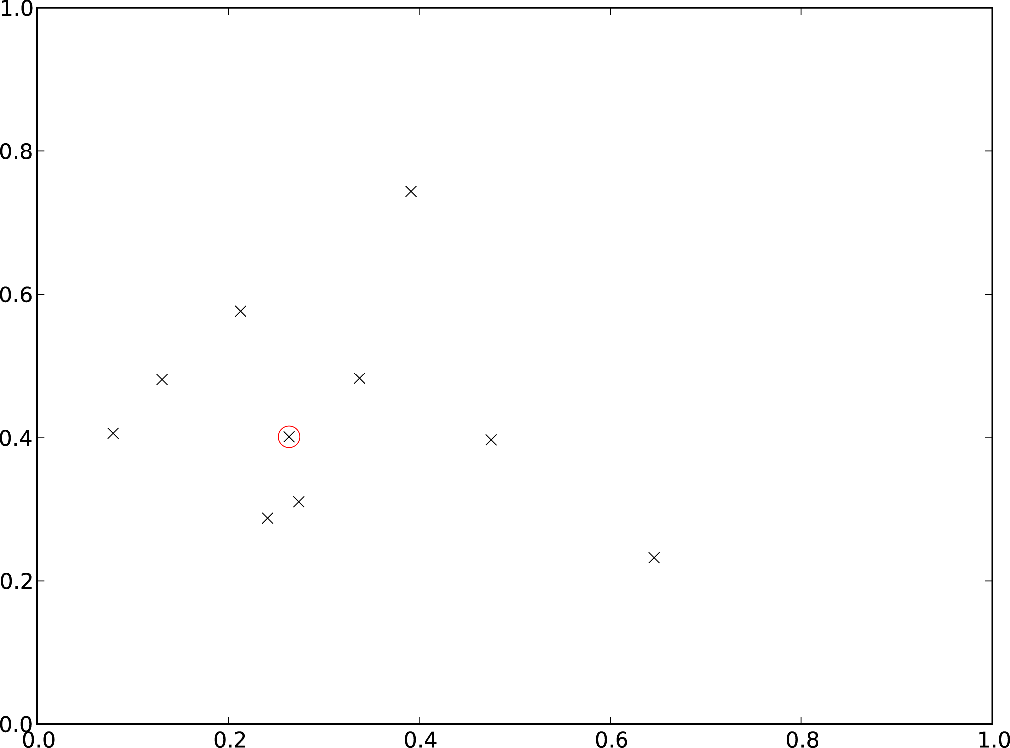
To illustrate the idea of the medoid,
Figure 1 shows the selection of a single medoid value from a set of 10 observations in a 2-dimensional space. The data is randomly generated, purely to give a visual representation of the concept. The point selected as the medoid, using
Equation (1), is circled in red. It shows how the selected point lies near the centre of the points in both dimensions.
The seasonal composites presented below are calculated using the medoid in the 6-dimensional space of reflectance values from the six Landsat reflective bands. However, other n-dimensional spaces could be used. For example, after processing reflectance data through the tasseled cap transformation [
16], one is presented with a 3-dimensional space of brightness, greenness and wetness, and one could apply the medoid in that space, to choose values which would be seasonally representative in terms of those three dimensions. Similarly, Scarth
et al. [
17] have defined a transformation from reflectance into fractional cover space, with three cover fractions representing the relative amount of cover of green vegetation, non-green vegetation, and bare soil. One could apply the medoid in this three-dimensional space, to obtain seasonally representative estimates of fractional cover. Another alternative would be to transform the reflectance values to alter the relative weight of different bands, or to leave out bands, which were felt to be irrelevant for a particular purpose. However, for the purposes of demonstrating the method, we have chosen to work with the untransformed surface reflectance in all six Landsat reflective bands. The applicability of this technique to other spaces would depend on the desired outcomes, and is beyond the scope of this article.
In estimating a value which is representative of the season, we choose to add a restriction on the number of input points. If a given pixel has less than three observations available for the season, after masking, we define the result as missing, on the principle that we do not have enough data to know how representative our choice might be. Neither the medoid nor the geometric median are robust against a single outlier in the case of less than three observations.
After a given date is selected for a given pixel, in a given season, the selected date is recorded, per pixel, and per season, so that the processing of every pixel can be tracked completely.
2.2. Quantifying “Representativeness”
Having used some method to select a point in multi-dimensional space which is to represent a group of such points, we need some way to quantify how representative the selected point is, in order to measure its performance against other methods. We have aimed for a measure which captures the intuitive notion that the seasonal value should follow the time series of single-date values, but should not be too readily influenced by outliers. Since the medoid is defined as minimizing a quantity of this sort in n-dimensional space, we have chosen to define a simpler measure, per band, in the interests of clarity. It is worth noting that to some extent this appears a little circular, since the medoid is more representative, in this sense, simply because of how it is defined. However, this test of “representativeness” provides a test of the extent to which the medoid, which is defined by choosing a point “in the middle” with respect to all dimensions simultaneously, results in values which are also ‘in the middle” in each dimension, independently of the other dimensions.
For each season, for each band, we calculate the seasonal average residual of the input data values after subtracting the selected representative value. If the selected point is representative in that band, then the individual residuals should be both positive and negative, and so the average should be close to zero. We present these seasonal residuals for the medoid and the MNC. We present example time series plots of these seasonal residuals, and also mean values across all pixels in the imagery. We also present the mean absolute value of the seasonal residuals, in order to check their absolute magnitude. Since the seasonal residuals can be both positive and negative, averaging over time and space could hide large residuals of both signs, whereas the mean absolute value will show these as large overall averages.
In formal terms, we define a seasonal residual
∊ in
Equation (2). For a given band, we have a set of
m single-date observations
yk for that band in a single season, and seasonal value
S which we have chosen as representative of that season for that band. We define the seasonal residual of
SWe calculate the mean seasonal residual
by averaging over all seasons, per pixel, and then averaging over all pixels. We calculate the mean absolute seasonal residual
by averaging |∊S| over all seasons, per pixel, and then averaging over all pixels.
The time series plots are given for both reflectance, and for NDVI calculated from the reflectance. The seasonal values for NDVI are calculated from the seasonal reflectance values.
An ideal choice for a value to represent the seasons should have small values for these averages, in all bands. This provides a basis for comparing methods of choosing the most representative value.
3. Data
All input Landsat TM/ETM+ imagery was downloaded from the USGS EarthExplorer website [
18] as level L1T imagery. Images which the EarthExplorer site rated as having greater than 80% cloud cover were not downloaded, on the assumption that they would contribute little, and would add extra noise in the form of undetected cloud, shadow, and mis-registration (which is a greater risk in very cloudy images). The imagery has been corrected for atmospheric effects, and bi-directional reflectance and topographic effects, using the methods detailed by Flood
et al. [
7]. The resulting imagery is expressed as surface reflectance. Cloud, cloud shadow and snow have been masked out using the Fmask automatic cloud mask algorithm [
10]. Topographic shadowing has been masked using the Shuttle Radar Topographic Mission DEM [
19,
20] at 30 m resolution, and the methods described by Robertson [
21].
Seasonal reflectance images are created for the combination of Landsat-5 TM and Landsat-7 ETM+ imagery, where both are available, on the assumption that the two instruments are sufficiently similar that the reflectance values can be treated as coming from a single population. Roy
et al. [
3] briefly discuss this possibility, and the radiometric details underlying this assumption are discussed a little further here in Section 5.
The examples shown are for the Landsat WRS-2 path/row 093/077, which is located in the Australian state of Queensland (see
Figure 2). This scene contains a mixture of vegetation cover types, with some eucalypt forest, some open pasture, and some cropping areas. Example time series graphs are given for two points within this image, one from a forested pixel and one from a grassland pixel. These two points are marked on the imagery in
Figure 3. Their locations are given in
Table 1. It should be emphasized that the time series graphs for these two points are presented purely as examples, to illustrate some of the behaviur which is possible over time. Quantitative analysis is performed on all pixels in the surrounding scene, over all dates. Other land types could show other characteristics, but an exhaustive global analysis is beyond the scope of the present demonstration article.
The chosen seasonal periods are September–November, December–February, March–May and June–August, corresponding to Spring, Summer, Autumn and Winter (in southern hemisphere terms). These are the same season boundaries as used by Roy
et al. [
3]. Trenberth [
22] gives a detailed discussion of what constitutes a season. Analysis is performed on all seasons for the period March 2000 to November 2012.
Also presented are seasonal mosaics of all scenes in the Australian state of Queensland, for the season March–May 2008, created using the medoid and the MNC.
4. Results
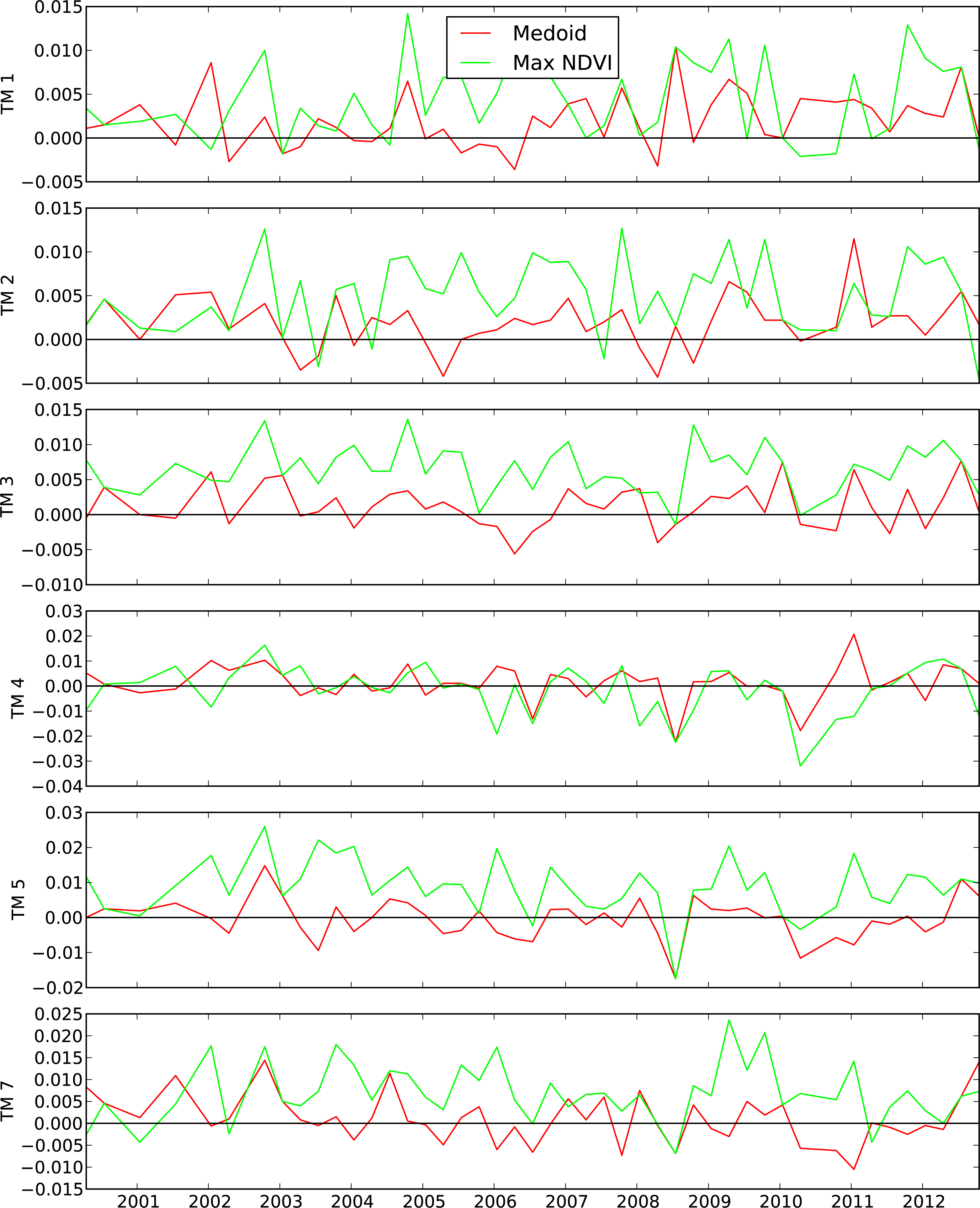
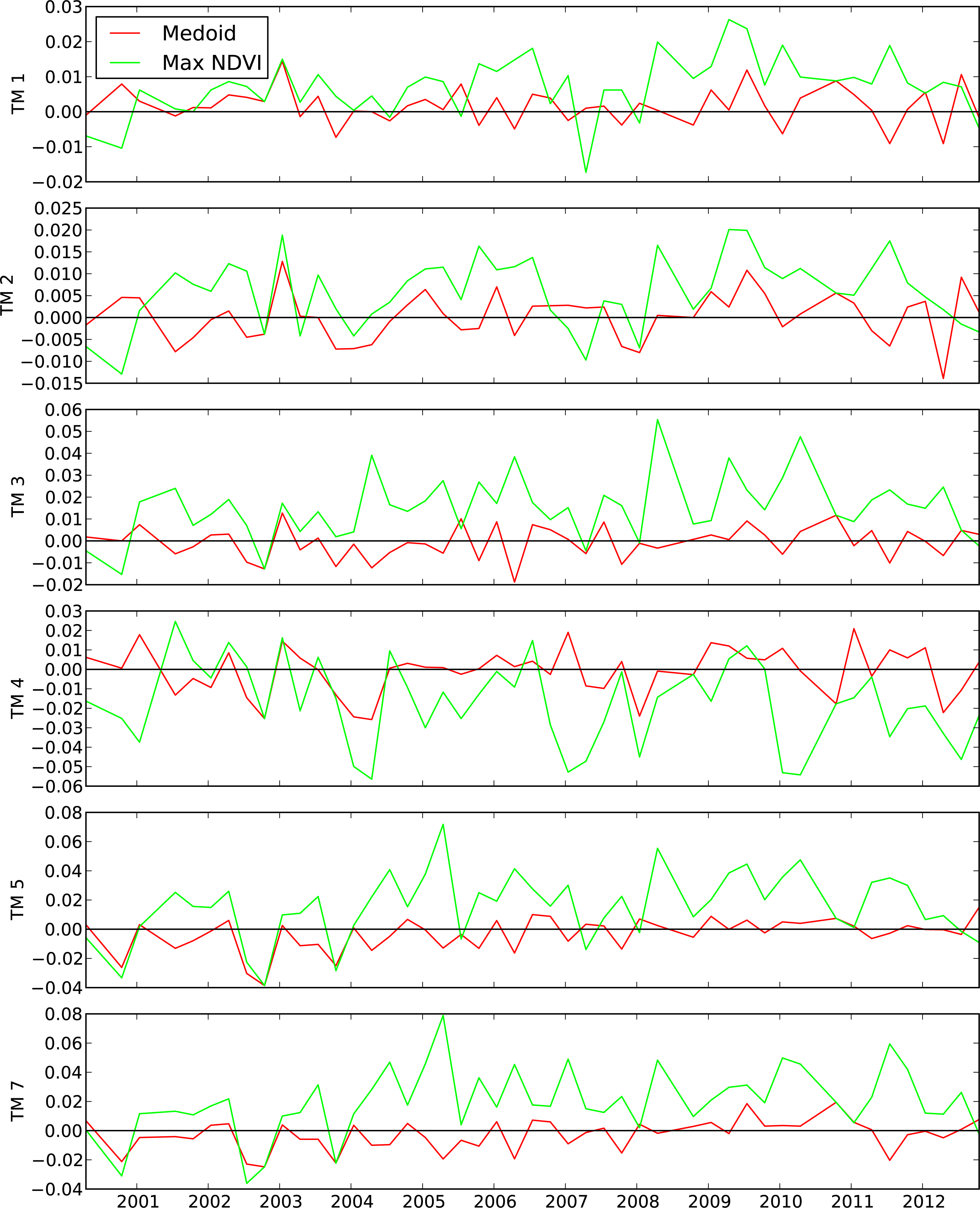
Figures 4 and
5 show the time series graphs of each reflectance band, for the two example points. The solid line shows the single-date values of reflectance. The marked points show the seasonally representative values, for medoid and MNC respectively. The seasonal values are positioned on the date for the centre of the relevant season.
Figure 6 shows the corresponding time series of NDVI values. The seasonal NDVI values are calculated from the corresponding seasonal reflectance values.
Figures 7 and
8 show the seasonal residuals for the reflectance values over time, on the two example pixels.
Table 2 gives average values for the residuals, averaged over time, and over all pixels in the WRS-2 path/row 093/077, for each Landsat TM/ETM+ band. The first two rows show the mean values of the residuals for the two different compositing methods. Since the seasonal residual values can be both positive and negative, and averaging such values can cancel out large residuals, we also show, in the next two rows, the mean absolute values of the residuals, for the two methods.
The final row attempts to quantify how often the medoid residual is larger than the MNC residual, by counting the percentage of seasons in which this occurs, averaged over all pixels.
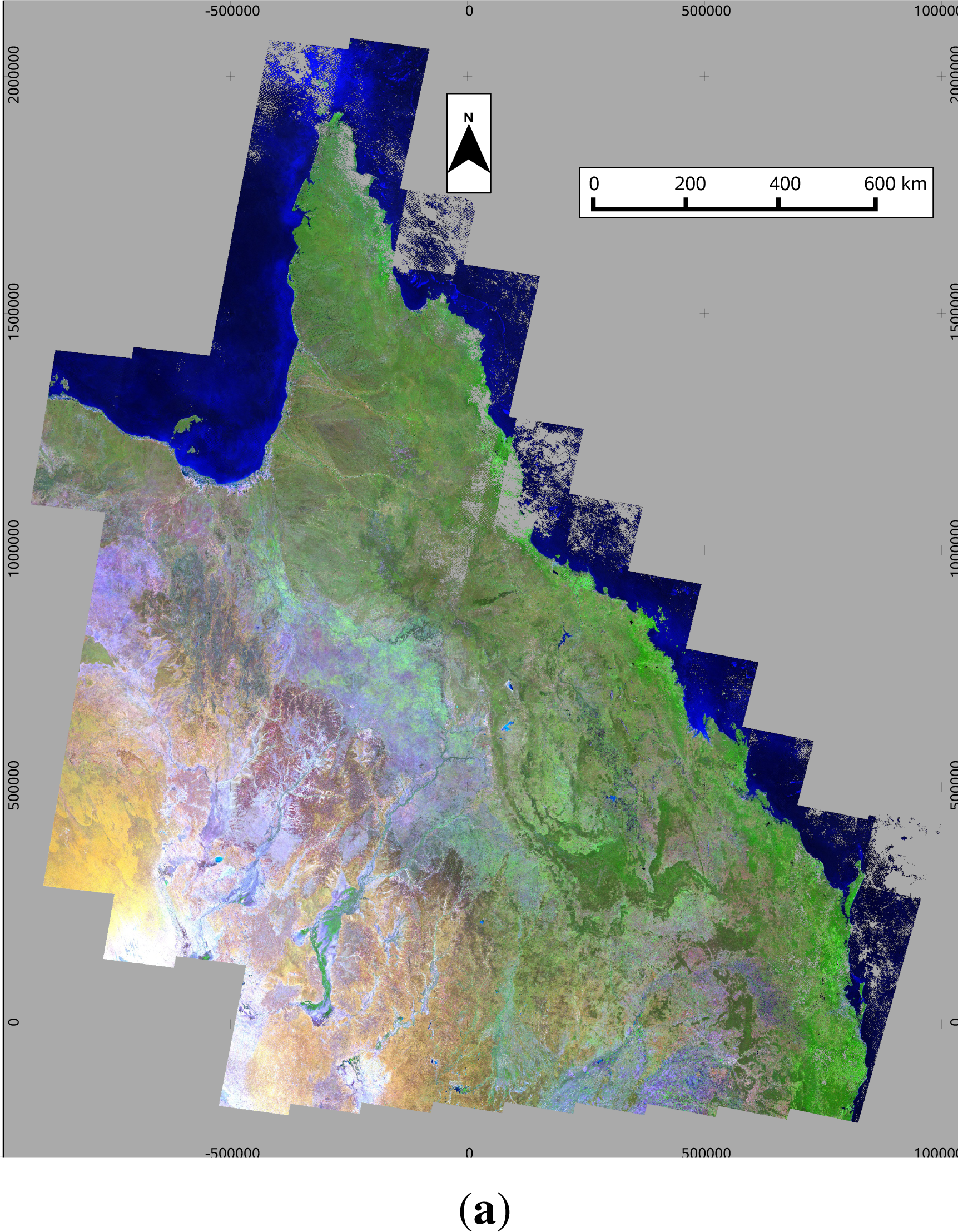
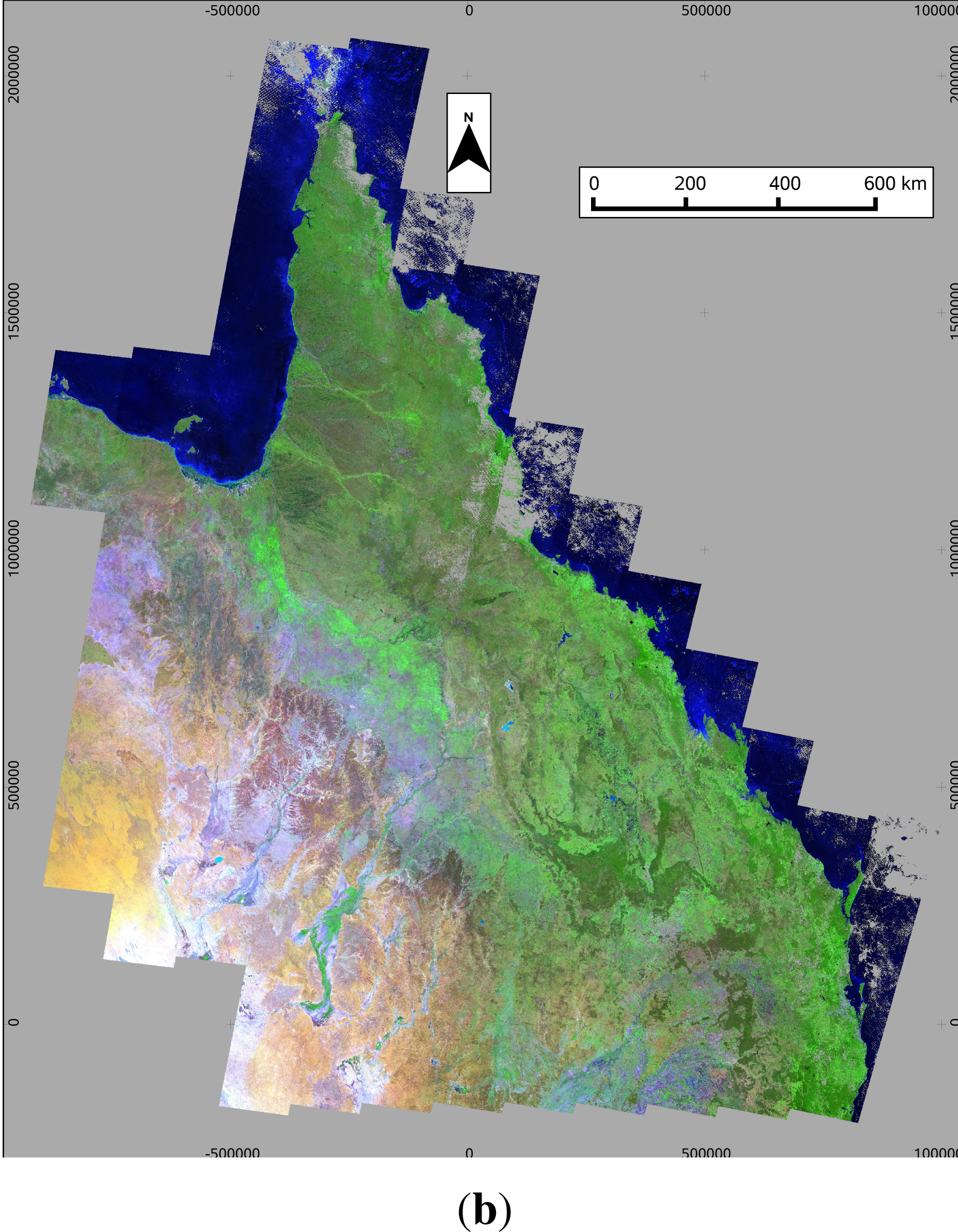
Figure 9 shows a seasonal mosaic of the Australian state of Queensland, for the season March–May 2008, produced using both methods under consideration. This covers a total of 102 WRS-2 path/rows.
Figure 9a was produced using the medoid, while
Figure 9b was produced using the maximum NDVI composite.
5. Discussion
Figures 4 and
5 illustrate the amount of variability in the individual images. However, they also illustrate that there also appears to be variability on longer time scales of seasons and years.
Figure 6 also shows this in the NDVI, with both locations showing clear evidence of annual cycles. In both the reflectance and the NDVI plots, visual inspection suggests that the medoid seasonal values follow the single-date values more closely than do the MNC values. In particular, as one would expect, the NDVI graphs illustrate the way the MNC favors the selection of higher NDVI, and misses much of the variation at the low-NDVI end.
Figures 4 and
5 also show that there are still outliers present in the data, even after the removal of cloud using automated masks, and correction for atmospheric and bi-directional reflectance effects. In most bands, the time series shows the presence of spikes in both directions, which would probably be caused by undetected cloud or cloud shadow, or imperfect correction for other effects. This should emphasize the importance of a measure which is robust against the presence of outliers.
The seasonal residuals shown in
Figures 7 and
8 show a little more clearly that the medoid follows the time series more closely. The medoid line (red) is generally closer to zero than the MNC line (green), although the graphs also illustrate that this is not so for every season.
The averages in
Table 2 summarize these effects over all pixels in all seasons for path/row 093/077. In order to conclude that the medoid provides a better estimate of the seasonal behavior, we would require that the average residuals have smaller magnitude, and that on average they should not be either consistently positive or negative. The averages given in
Table 2 show this to a marked degree, with the medoid residuals being up to an order of magnitude smaller than those for the MNC. We would also like to see that this is the case not just on average, but in at least the majority of seasons, and the final row of the table shows that it is true for the overwhelming majority of seasons (between 78% and 89%). This suggests quite strongly that the medoid seasonal values are, in general, a substantially better representation of the reflectance for the season than the MNC seasonal values.
Figure 9 shows two seasonal reflectance mosaics for the Australian state of Queensland, for the season March–May 2008 (autumn). The bands shown are TM bands 5, 4 and 1 as red, green and blue, respectively.
Figure 9a shows the seasonal values produced using the medoid, and for comparison,
Figure 9b shows the same mosaic produced using the MNC. The null value is shown as grey, indicating areas where fewer than three dates were available after masking for cloud and shadow. In both cases, the same three date minimum was used, which means the same areas are shown as missing in both (mostly due to persistent coastal cloud). Both mosaics are essentially seamless, showing that they have both captured a consistent pattern across scene boundaries, despite the fact that different paths are viewed on different dates. The main thing distinguishing them is the presence of higher levels of green vegetation in many areas in the MNC image, reflecting the bias towards higher NDVI. This would vary, depending on season and location.
Because we have required a minimum of three dates in a season before we will estimate a seasonal value, there are still some seasons when some pixels would have missing data. Given the occurrence of cloud in some areas, it can even be that case that there are no observations at all during a season, so any use made of the data must always be capable of dealing with missing data. However, the choice of a minimum of three dates was somewhat arbitrary, providing a balance between maintaining a robust estimate for the season, and not having too much missing data. In a season of 90–92 days, with a Landsat revisit interval of 16 days, one can expect to have either 5 or 6 observations from a single Landsat satellite (before losses due to cloud), and roughly double that when two satellites are combined. A minimum number of dates larger than three could be used, but this would result in more missing data in the result. It should be noted that if the minimum number of dates is less than three, then the result is no longer robust against the presence of a single outlier in the data.
As noted in Section 2.1, the medoid is robust against outliers until at least half of the points are to be considered as outliers. One obvious situation in which this would occur is when there is undetected cloud in more than half of the observations. This is in contrast to the behavior of the MNC, which is resistant to the presence of cloud so long as there is at least one cloud-free observation, because the MNC always selects against cloud (although the same is not necessarily true of other types of contamination, such as cloud shadow). This point highlights the need for at least the majority of cloud and other contamination to have been removed prior to application of the medoid.
Since May 2003, Landsat-7 has suffered from a failure of the Scan Line Corrector (SLC), which causes a loss some pixels from the image, predominantly near the edges of the path. The missing data is in the form of very long wedges running from the edges of the path towards the centre. The wedges are 14 pixels wide at the edge, and narrow to less than one pixel wide by around 11 km from the centre of the path. The nett loss of data is around 22% of the image [
23]. The 22 km wide strip in the centre is unaffected. This means that the edges of each path will have less data for the season than the centre. However, by including in the calculation the values from adjacent paths, we can double the amount of data available, and so these areas then become the most robust part of the seasonal image, with up to twice as much data as the rest of the scene. This rather fortuitously compensates for the SLC-off losses at the edges. However, missing data due to cloud is an issue across the whole scene, and there are cases in which a season has enough cloud during the season that most of the scene does not meet the three-date minimum, except in these overlap areas. The benefit of using the overlaps can be clearly seen in the mosaics in
Figure 9, in the area of persistent cloud on the north-east coast. Most of this area did not meet the three date minimum, but there is a strip of data from the overlap area running through the middle of it (easting, northing = 0, 1100000), which did meet the criterion. Because of the increased overlap between paths in higher latitudes, this effect will be of even greater benefit further from the equator.
During the period 2003–2011, imagery is available for both Landsat-5 TM and Landsat-7 ETM+. As noted in Section 3, we have chosen to mix these together as a single dataset, so that for a given pixel, either instrument can be selected. This notion has also been proposed by Roy
et al. [
3]. Whether this is appropriate would depend on the uses made of the resulting composite. If a user were performing a calculation which was sensitive to differences between the instruments, it may be necessary to record, per pixel, which instrument was selected, so that the appropriate form of calculation could be performed accordingly. The current work has kept such a record, as it would seem generally useful. There may also be cases when it is completely inappropriate to mix the sensors. However, in general terms the instruments are designed to be broadly compatible, and the composites created from the mixture of the two have the virtue of being derived from twice as many observations. Markham and Helder [
24] review the whole topic of creating consistency in calibration of the various Landsat sensors, and Teillet
et al. [
25] present a detailed analysis of the radiometric differences between Landsat-5 TM and Landsat-7 ETM+.
The quantitative analysis presented in
Table 2 is for all dates and pixels of a single path/row, in eastern Australia. However, given the definitions of the medoid and the MNC, it seems likely that the same relative behavior would be apparent in any other location. In particular, the MNC’s bias towards greener dates would be present, unless there was little variation in NDVI across the season, in which case the medoid and the MNC would generally give much the same result.
It should also be re-emphasized that the use of the medoid in this way does depend on the removal of most of the contamination from other sources. All of the various methods currently in use for doing so are imperfect, but only by reducing the incidence of significant contamination to a minority of dates can one reasonably expect the medoid to then select against what remains. The accuracy statistics quoted for cloud and shadow removal suggest that this is now possible for those contaminants. Ju
et al. [
26] suggest that the same may not be true for some methods of aerosol estimation. Tests by Gillingham
et al. [
27] suggest that the methods used in this study [
7] may be sufficient in the Australian context, however, this is largely due to the fact that Australia frequently has very low aerosol loadings (by global standards). Before applying these ideas in other locations, one should consider this issue carefully in the local context.
6. Conclusion
We have proposed an alternative approach to the creation of multi-temporal composites images, based around the medoid. Because of improvements in other aspects of image pre-processing, the need for the maximum NDVI composite method (MNC) to actively select against some types of data contamination is now reduced, and this has enabled the use of more representative estimates of seasonal values.
We define what we mean by a seasonal value being “representative” of the data for that season, in terms of the average residual value for the season. Analysis of these seasonal residuals suggests that the medoid-based seasonal values are more representative of the underlying time series than the seasonal values produced by the MNC algorithm. The medoid-based seasonal values also avoid the tendency of the MNC to bias in favor of high NDVI observations. This is just what one would expect, given the definition of the medoid and the MNC. While the quantitative analysis presented here is limited to the time series of images on a single path/row, there seems little to suggest that this would behave radically differently on any other path/row.
The resulting seasonal time series is on a regular time interval (4 seasons per year), and is very robust against contamination from a range of sources.
As discussed in the introduction, the main intention of creating such seasonal composites is a regular time series of reflectance imagery which captures the temporal variability on a seasonal time scale. The value of such a time series would depend on the application. Plainly, if one required information on variability at shorter time scales than this, one would not be able to use a seasonal composite. Indeed, the sampling theorem demonstrates that the highest temporal frequency which can be represented in a regularly sampled signal is half the sampling frequency [
28,
29]. Using the techniques outlined here for shorter time scales would be problematic because of the reduce number of dates in shorter periods, leading to increases in the frequency of insufficient dates to create a medoid.


