A Satellite-Based Surface Radiation Climatology Derived by Combining Climate Data Records and Near-Real-Time Data


Abstract
: This study presents a method for adjusting long-term climate data records (CDRs) for the integrated use with near-real-time data using the example of surface incoming solar irradiance (SIS). Recently, a 23-year long (1983–2005) continuous SIS CDR has been generated based on the visible channel (0.45–1 μm) of the MVIRI radiometers onboard the geostationary Meteosat First Generation Platform. The CDR is available from the EUMETSAT Satellite Application Facility on Climate Monitoring (CM SAF). Here, it is assessed whether a homogeneous extension of the SIS CDR to the present is possible with operationally generated surface radiation data provided by CM SAF using the SEVIRI and GERB instruments onboard the Meteosat Second Generation satellites. Three extended CM SAF SIS CDR versions consisting of MVIRI-derived SIS (1983–2005) and three different SIS products derived from the SEVIRI and GERB instruments onboard the MSG satellites (2006 onwards) were tested. A procedure to detect shift inhomogeneities in the extended data record (1983–present) was applied that combines the Standard Normal Homogeneity Test (SNHT) and a penalized maximal T-test with visual inspection. Shift detection was done by comparing the SIS time series with the ground stations mean, in accordance with statistical significance. Several stations of the Baseline Surface Radiation Network (BSRN) and about 50 stations of the Global Energy Balance Archive (GEBA) over Europe were used as the ground-based reference. The analysis indicates several breaks in the data record between 1987 and 1994 probably due to artefacts in the raw data and instrument failures. After 2005 the MVIRI radiometer was replaced by the narrow-band SEVIRI and the broadband GERB radiometers and a new retrieval algorithm was applied. This induces significant challenges for the homogenisation across the satellite generations. Homogenisation is performed by applying a mean-shift correction depending on the shift size of any segment between two break points to the last segment (2006–present). Corrections are applied to the most significant breaks that can be related to satellite changes. This study focuses on the European region, but the methods can be generalized to other regions. To account for seasonal dependence of the mean-shifts the correction was performed independently for each calendar month. In comparison to the ground-based reference the homogenised data record shows an improvement over the original data record in terms of anomaly correlation and bias. In general the method can also be applied for the adjustment of satellite datasets addressing other variables to bridge the gap between CDRs and near-real-time data.1. Introduction
In light of the growing need for long-term climate data sets to understand climate variability and change, substantial international efforts have been made in recent years. In 2008, a network of agencies and operators of environmental satellites, called “Sustained, Coordinated Processing of Environmental Satellite Data for Climate Monitoring” (SCOPE-CM) [1], was established for the coordination of the sustainable generation of long-term Climate Data Records (CDR). These records built upon Essential Climate Variables (ECV) as defined by the Global Climate Observing System (GCOS). SCOPE-CM interface with the WMO Integrated Global Observing System (WIGOS) and the Global Space-based Inter Calibration System (GSICS), building an end-to-end system for climate monitoring [2].
CDRs are time series of climate variables accounting for systematic errors and noise in the measurements (NRC 2004). They comprise homogeneous long-term data records of radiances or brightness temperatures (Fundamental Climate Data Records, FCDR) and their derived geophysical variables (Thematic Climate Data Records, TCDR). The mandatory requirements for CDRs are accurate calibration and high stability over time [3]. This calls for careful treatment of the data and sophisticated methodologies which is, in practice, time-consuming and demands high computational capacities. CDRs are generally results of long-lasting reprocessing activities and hence the latency of product releases or updates is several years.
A better timeliness of climate data is enabled by the provision of so called Environmental Data Records (EDR), which are constructed as instantaneous estimates of geophysical variables [4]. EDRs are generally provided in operational mode in near-real-time and do not meet the strict requirements made for CDRs. They generally lack stability, accuracy and sufficient length for climate studies. However, EDRs are built from the newest generation of satellite instruments and are per se capable of measuring the respective climate variable with the highest possible precision.
Climate research and climate monitoring can therefore not exclusively rely on satellite data not considering recent years but rather need data on an ongoing basis and hence require the generation of CDRs in near real-time. Trenberth et al. [5] point out the discrepancy between the release of IPCC assessments (every six or seven years) and the need for short term assessments of the current climate. The authors state that “near-real time information and attribution is increasingly in demand, especially when major events occur”.
Recently, some effort has been made to bridge the gap between long-term data sets and near-real time data. For instance, AghaKouchak and Nakhjiri [6] use Bayesian correction for the creation of a long-term CDR of drought using a method proposed by Tian et al. [7] for the real-time bias reduction of precipitation data.
Generally, the combination of different datasets addressing one single variable is subjected to several problems which are related to different instruments, algorithms and data providers. Liu et al. [8] describe the combination of various types of satellite instruments ranging from active to passive sensors for the retrieval of soil moisture estimates, with emphasis on preserving long term trends. Comiso and Nishio [9] describe the generation of a sea ice cover dataset using three different instruments.
The current paper presents a method for the adjustment of CDRs for the integrated use with near-real time data, using datasets for global radiation, provided by the EUMETSAT Satellite Application Facility on Climate Monitoring (CM SAF). Global radiation has been chosen due to its role as a crucial player in the global climate system and the large efforts that have been made particularly on the homogenization of surface radiation datasets in the past.
Moreover, surface radiation estimates from satellite-based sensors have become indispensible in a wide range of applications, such as the planning of photovoltaic systems (e.g., [10]), as an important input for climate models in hydrological and climatological applications (e.g., [11]), to derive climate variables such as evaporation (e.g., [12]) and to monitor the climate system (e.g., within the WMO Regional Climate Centre on Climate Monitoring for Europe and the Middle East [13]).
Recently, the Satellite Application Facility for Climate Monitoring (CM SAF) created a 23-year long CDR of surface solar radiation parameters including solar surface irradiance (SIS) and direct irradiance (SID) for the period 1983–2005 [14,15] based on measurements of the Meteosat Visible and Infrared Imager (MVIRI) radiometer onboard the geostationary Meteosat First Generation (MFG) satellites. This dataset has been created using a self calibration algorithm to automatically compensate for the degradation of satellite sensors and discontinuities in the SIS CDR due to changes between different satellite instruments. The satellite-derived SIS shows high anomaly correlations (r = 0.89) and a small positive bias of +4.4 W·m−2 compared with ground-based measurements by 12 stations of the Baseline Surface Radiation Network (BSRN) [14]. In addition, the SIS CDR was found to be homogeneous for the time period covered by observations from the BSRN stations (restricted to the period after 1990). An intercomparison with similar datasets including the International Satellite Cloud Climatology project (ISCCP; [16]), the Global Energy and Water Cycle Experiment (GEWEX; [17]), and the European Center for Medium-Range Weather Forecasts reanalysis dataset ERA-Interim [18] indicated lower bias and higher anomaly correlation of the CM SAF dataset with most of the BSRN stations.
Brinckmann et al. [19] performed an extensive homogeneity analysis of the SIS CDR for the period 1983–2005 using five BSRN stations and ECMWF’s ERA-Interim reanalysis as reference. They found particular inhomogeneities in comparison to ERA-Interim in a short period between 1988–1990, when the problematic Meteosat-3 satellite was in use for two short time intervals. Over Europe, further inhomogeneities were mainly found before 1994 and could be attributed to satellite changes. Sanchez-Lorenzo et al. [20] performed a comprehensive analysis of the CM SAF SIS CDR over Europe for the period 1983–2005 using 47 ground-based observations by the Global Energy Balance Archive (GEBA) as the reference and also found the SIS CDR to be inhomogeneous only before 1994.
The shift inhomogeneities before 1994 may be related to stripes in the raw satellite data, which are interpreted as cloudless areas by the retrieval algorithm and hence lead to an increase of SIS. The temporal stability of the SIS CDR after 1994, however, indicates that homogeneous data can be generated from satellite observations across instrumental changes, and it is a matter of the applied retrieval method and data filtering to generate a homogeneous time series.
The SEVIRI instrument onboard MSG does not provide broadband channel observations for the full disk. Hence, the full disk dataset derived from the MVIRI instrument on MFG cannot be directly homogeneously extended with SEVIRI observations. In order to examine the effect of using narrowband channels instead of broadband Posselt et al. [14] investigated the difference in the derived SIS using the overlapping period of Meteosat 7 (MFG) and Meteosat 8 (MSG; 2004–2005). Posselt et al. [14] showed that the use of one of the narrowband channels of Meteosat-8 induces significant differences in SIS and hence inhomogeneities in specific areas. Particularly over densely vegetated areas (South America, tropical Africa and Europe during the summer months) significant differences were found.
The current paper examines, in the first part, the temporal homogeneity of three extended versions of the CM SAF SIS CDR based on observations from MVIRI on the MFG platforms (1983–2005) and three slightly different SIS datasets derived from MSG measurements by the Geostationary Earth Radiation Budget (GERB) and/or the SEVIRI instruments (2006 onwards). Thereby, observations by the BSRN and the GEBA network serve as ground-based reference. In the second part, a procedure to detect the breakpoints was applied, which combines the Standard Normal Homogeneity Test (SNHT; [21]) and the penalized maximal T-test (in the following referred to as RH test; [22,23]) with visual inspection. Thereby, the extended SIS CDR was compared with individual stations and the station average of the ground-based reference network. Europe constitutes the world’s highest density of surface-based SIS observations [24], and was therefore selected to demonstrate the proposed methodology. Homogenisation was done by applying a mean-shift correction between any segment (e.g., the time series between two breakpoints) and the last segment (2006 onwards), which were determined using the difference series between CM SAF and the ground-based reference. The statistical relationship between the station-wise determined mean-shifts and the difference between MFG- and MSG-based SIS in the overlap period (April–December 2005) was used to correct the satellite estimates at locations where a ground-based reference was unavailable. The performance of the applied method is demonstrated comparing the adjusted satellite estimates to the ground-based reference and to the MSG-based SIS in the overlap period.
2. Data
2.1. The CM SAF datasets
The satellite-derived datasets used in the present study are based on data obtained from EUMETSAT’s geostationary Meteosat satellites of the First and Second Generation (MFG and MSG). The CM SAF provides a SIS CDR (1983–2005) based on observations from the Meteosat Visible and InfraRed Imager (MVIRI) instruments onboard the MFG satellites. The MVIRI radiometer senses the earth’s disc with a frequency of 30 min in three channels covering visible and near infrared radiances. The broadband visible channel (0.45–1 μm) used for the retrieval of SIS has a spatial resolution of 2.5 km at nadir.
Here, the MVIRI-derived SIS CDR (1983–2005) is temporally extended to the present with three different CM SAF MSG products, which are based on the Geostationary Earth Radiation Budget (GERB) and the Spinning Enhanced Visible and Infrared Imager (SEVIRI) onboard the MSG satellites. One dataset is the operational CM SAF product, provided in near-real-time on a monthly base (MSGG). The other two products are currently in a development stage (MSGGL and MSGS). Table 1 provides an overview over the different algorithms and satellite data used for the generation of the different SIS data sets.
Compared to the MVIRI sensor, the SEVIRI instrument has a higher frequency of observations (every 15 min) and more spectral channels (12). The narrow-band visible channels are centered at 0.6 μm and 0.8 μm, and have a slightly lower spatial resolution than the MVIRI instrument of 3 km at nadir. In addition, SEVIRI contains a broadband High-Resolution-Visible channel (HRV) that corresponds to the MVIRI broadband visible channel, yet with a higher resolution of 1 km at nadir. However, the HRV channel does not cover the full disc, and cannot be used to extend the SIS CDR.
The original Heliosat algorithm [25,26] uses the digital counts observed by the MVIRI sensor to determine the effective cloud albedo, which is combined with estimated clear-sky radiances using clear-sky model MAGIC (Mesoscale Atmospheric Global Irradiance Code; [27]) to calculate the satellite-derived SIS. For the generation of the CM SAF SIS CDR, the Heliosat algorithm was modified to include a self-calibration parameter to minimize the impacts of satellite changes and artificial trends due to degradation of satellite instruments. The self-calibration uses a cloudy target region in the southern part of the South Atlantic, the 95th percentile of the radiances observed in this region is used as basis for the self-calibration (see [28] for details). In addition, a seven-day running mean is applied to obtain the clear-sky background field instead of monthly mean values [29]. The MVIRI-derived SIS dataset is abbreviated as MFG in the following.
Posselt et al. [30] recently combined the two visible channels of SEVIRI following a linear combination proposed by Cros et al. [31] and applied the same Heliosat-approach as for the generation of the CM SAF SIS CDR to provide a SIS dataset covering 2004 to 2010.This SEVIRI-based SIS dataset is referred to as MSGS in the following.
The operationally generated MSG-based SIS dataset from CM SAF (MSGG) uses a look-up-table approach to relate the observed radiance at TOA with the surface radiation [27] using SEVIRI and GERB data. This data is continuously generated and provided on a regular basis. MSGG uses a new GADS [32]/OPAC [33] aerosol climatology, which is optically denser than the aerosol climatology used for MFG [34] and is a potential source for inhomogeneities across the satellite generations.
The third MSG-based SIS CDR used in this work (MSGGL) also applies a Heliosat approach, however, here a classical minima approach for clear sky reflection is used instead of fuzzy logic. GERB-like data are used to derive the SIS, which are calculated from SEVIRI and adjusted to GERB.
2.2. Validation Datasets
The satellite-derived SIS is evaluated using ground-based stations from the Baseline Surface Radiation Network (BSRN) and the Global Energy Balance Archive (GEBA), which are introduced in the following.
2.2.1. BSRN Data
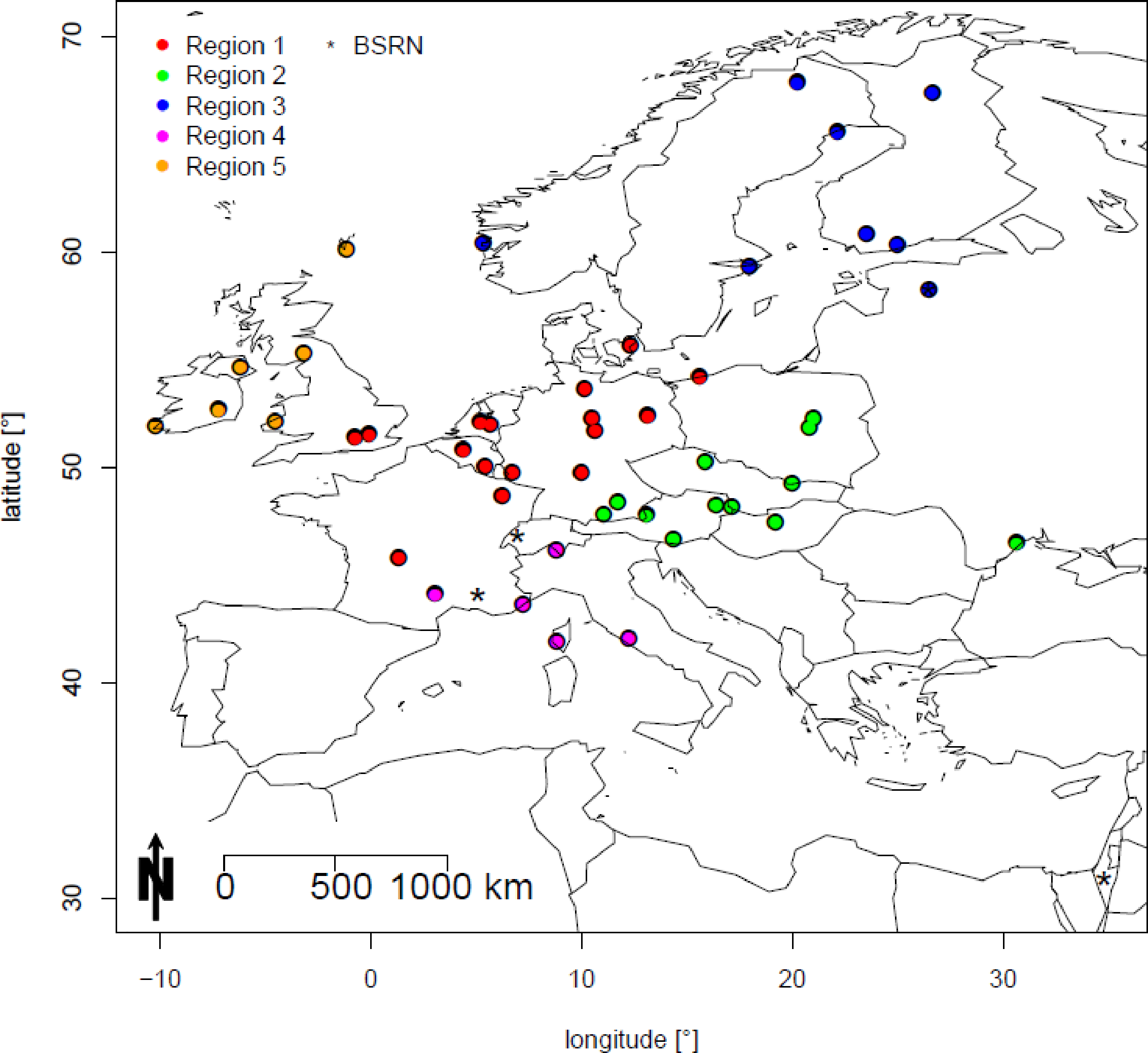
BSRN is a project of the Global Energy and Water Experiment (GEWEX) and the World Climate Research Program (WCRP) [35]. BSRN provides currently data from about 50 globally-distributed quality-controlled surface radiation measurements site of high consistency applying a defined set of sensors and measurement protocols. The accuracy of the SIS observations is estimated to be about 5 W·m−2. Here, we used SIS data of four stations with time series covering the period 1995–2010 (Payerne, Toravere, Carpentras and Sede Boquer; Figure 1). These data served as a reference to evaluate the quality of the satellite-derived SIS for the period around the instrumental change from MVIRI to GERB and SEVIRI.
2.2.2. GEBA Data
In addition to the BSRN stations SIS measurements obtained from the GEBA were used, as they provide a larger database often dating back to the 1960s. The GEBA database is maintained at the ETH Zurich, which collects worldwide monthly means of several surface energy flux measurements [36] with the highest station density over Europe. Sanchez-Lorenzo et al. [20] compiled a set of homogeneous, long-term SIS series over Europe. The final dataset consists of 56 station series, with the highest station density over Central Europe. The datasets have been quality checked using a method by Aguilar et al. [37] to remove outliers and unrealistic values from the SIS series. In addition the SIS series have been tested for temporal homogeneity using the Standard Normal Homogeneity Test (SNHT; [21]), with monthly adjustments being applied to the most significant breaks only. As the GEBA stations cover a large fraction of the observing period of the diverse Meteosat satellites, they are an ideal reference to check the satellite-derived SIS for temporal consistency.
Following Sanchez-Lorenzo et al. [20], the validation of the CM SAF dataset was based on a subset of 47 homogenised and filled GEBA stations over Europe over the period 1983–2007 (Figure 1). In addition, the validation was performed for regional mean series and multisite means. The use of the mean series improves the detection of weak signals as it enhances the signal-to-noise ratio and reduces the impact of possible inhomogeneities in the reference series. The regionalisation of the 47 GEBA stations was adopted from Sanchez-Lorenzo et al. [20] and bases on Principle Components Analysis that clusters the stations into regions with similar temporal variability.
3. Methods
A procedure to detect shift inhomogeneities in the extended CM SAF data record (1983–present) was applied that combines the Standard Normal Homogeneity Test (SNHT) and a penalized maximal T-test with visual inspection. The calculation of the adjustments is based on the mean-shifts of the difference series (CM SAF minus BSRN/GEBA) at a breakpoint to the reference segment (the segment after 2006). Correction at every grid point was performed by relating the station-wise determined mean-shifts to the difference field (e.g., MSG-minus MFG-based SIS) in the overlap period of both datasets (April to December 2005) and the geographical coordinates. Section 3.1 introduces the applied homogeneity tests for the detection of breakpoints and Section 3.2 the mean-shift adjustment applied to the CM SAF SIS CDR.
3.1. Homogeneity Tests
Several studies recently assessed the quality of the CM SAF SIS CDR against ground-based reference datasets [19,20,29]. In these studies the CM SAF SIS CDR was found to be homogeneous in Europe over the period 1994 to 2005, while some shifts and artificial trends were detected before 1994.
Here, the extended datasets (see Section 2.1) consisting of both the MFG- and the MSG-based SIS was assessed for possible shift inhomogeneities over the European region. For this purpose, the Standard Normal Homogeneity Test (SNHT; [21]) and the penalized maximal T-test [22] were applied to the difference series between the CM SAF and the GEBA SIS anomalies. The homogeneity analysis was performed using monthly SIS anomalies to remove seasonal variability. The tests were applied to the difference series of individual stations and of the station average. The use of the mean series improves the detection of weak signals as it enhances the signal-to-noise ratio, and it reduces the impact of possible inhomogeneities in the reference series. In addition, we assumed that inhomogeneities due to changes in satellite instrumentation and in the applied retrieval algorithms occur over the whole Meteosat disc. Table 2 provides an overview over major events that may have affected the stability of the CM SAF SIS CDR. Switches between satellites for only a few days are not listed (see details in [38]).
3.1.1. Standard Normal Homogeneity Test
The SNHT test detects shifts and artificial short-term and long-term trends in a time series. The test value T(k) is calculated for each time step k of the investigated time series.
and are determined using the mean Ȳ and the standard deviation s of the tested time series:
Large dissimilarities of and indicate a mean-shift at k, which leads to high values of T(k). In the case T(k) exceeds a certain level Tc, which depends on the chosen significance level and the length of the considered time series, a break point is detected at T0 = max(T(k)). Here, the Tc values for the 95%-significance level are adopted from Brinckmann et al. [19].
3.1.2. RH Test
Besides the SNHT test, also the RH test [22] was applied to the time series for the detection of multiple breakpoints, in order to enhance the confidence in the detected breaks. A major shortcoming of the SNHT test is its uneven distribution of false alarm and detection power depending on the position in the time series, which is alleviated by using an empirical penalty function. In addition, the RH test accounts for first order autocorrelation in the tested time series [22], which enables the detection of multiple break points in a series. The most probable position of the break point is derived by maximizing T(k):
3.2. Mean-Shift Adjustment
After the identification of the significant breakpoints, a mean-shift based adjustment was applied to the time series to remove the artificial shifts. The correction was applied to time series between two breakpoints (in the following referred to as segments) that were significant on the 95% level for a large fraction of individual difference series and for the mean difference series, and that could be related to changes in satellite instrumentation or retrieval algorithm.
3.2.1. Calculation of the Mean-Shift Adjustments
A correction was applied to the identified breaks based on the mean-shifts that were calculated from the difference series (CM SAF minus GEBA). The mean-shifts correspond to the fitted mean response of the difference series (CM SAF minus GEBA) at a breakpoint to the reference segment (the segment after 2006). Due to the observed strong seasonal dependency of the difference between MFG- and MSG-based SIS [14], the mean-shift adjustment varies for each month. Time series for each calendar month (covering the period 1983–2007) were generated, and the shift sizes were determined separately for each month.
3.2.2. Application of the Mean-Shift Adjustments to the European Region
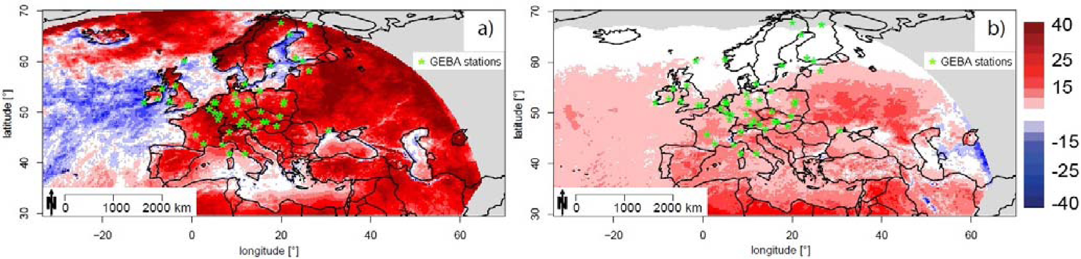
The overlap period (April to December 2005) of the operationally derived MSGG from Meteosat 8 and the SIS derived from Meteosat 7 (MVIRI) was used to determine the shifts in the CM SAF dataset that result from changes in the satellite instrumentation and the retrieval algorithm. The SIS difference between the two datasets (e.g., MSG- minus MFG-based SIS; henceforth referred to as the difference field) is characterized by a distinct pattern over Europe (Figure 2), which is mainly governed by the seasonal variation of the solar zenith angle and the land-sea distribution. To remove fluctuations in the annual cycles of both the station-wise derived mean-shifts and the difference field due to measurement uncertainties in both datasets a smoothing spline function with six degrees of freedom was applied.
We found good correlations between the station-wise determined mean-shifts and the difference field at the grid points closest to the ground-based stations in the overlap period. The similarity of the station-wise detected mean-shifts and the difference field was used to transfer the mean-shifts derived for each station to every grid point within the European region. Thereby, for each calendar month separately, the station-wise determined mean-shifts were linearly regressed using the difference field (in the overlap period) and the geographical coordinates as predictors.
4. Results and Discussion
This section starts with the validation of the three extended CM SAF SIS CDR versions consisting of MVIRI-derived SIS (1983–2005) and three different SIS products derived from the SEVIRI and GERB instruments onboard the MSG satellites (2006 onwards) (see Section 2.1). The CM SAF SIS dataset that compares best with the ground-based reference measurements was selected for further investigations. In a next step, the homogeneity tests described in the previous section were applied to 47 difference series (CM SAF minus GEBA) to inspect the temporal stability of the extended CM SAF SIS CDR from 1983 to 2007. The performance of the applied adjustments was assessed in comparison with the 47 GEBA series. Finally, the impact of the proposed correction scheme on every grid-point was demonstrated by examining the corrected CM SAF SIS CDR.
4.1. Validation of the Extended CM SAF SIS CDRs
The validation was performed using 47 GEBA stations for the period 1983–2007 and four BSRN stations for the period 1990–2010 as ground-based reference over Europe. The validation was conducted for each time series individually; in addition a multisite mean was calculated by averaging the station-wise derived values. Several statistical measures were calculated such as the bias, the mean absolute error (MAE), the standard deviation of differences (SDD), and the anomaly correlation (AC). The applied quality measures are defined in the Appendix.
Tables 3 and 4 summarize the validation results for the monthly means of the CM SAF SIS at the BSRN and the GEBA station, respectively. The MAE of MFG is well below the targeted accuracy threshold of 15 W·m−2. The requested accuracy was exceeded for only 11.4% of the monthly data if compared to BSRN (Table 3) and in 15.6% of all cases if compared to GEBA (Table 4). The high anomaly correlation of 0.84 with BSRN and 0.87 with GEBA as reference demonstrates the excellent agreement at the monthly scale of the CM SAF data and the surface measurements. The slightly different results obtained using either BSRN or GEBA as ground-based reference highlight the impact of the selected reference stations in terms of station locations and measurement uncertainty. This also explains slightly differing validation results found in previous studies (see [20,29]).
Also included in these tables are the corresponding values for sub-periods of the MFG and the three MSG datasets. All CM SAF datasets have a high quality as documented in MAE well below 10 W·m−2. MSGS was most consistent with MFG for most of the applied quality measures, which can be explained by the use of consistent input satellite data and retrieval algorithm. MSGG yielded the smallest bias and mean absolute error (−1.28 W·m−2 and 8.68 W·m−2 compared to GEBA, respectively) of all datasets. The difference between the MSG data sets are due to differences in the used satellite data and applied retrieval methods, see Table 1 for details about the difference.
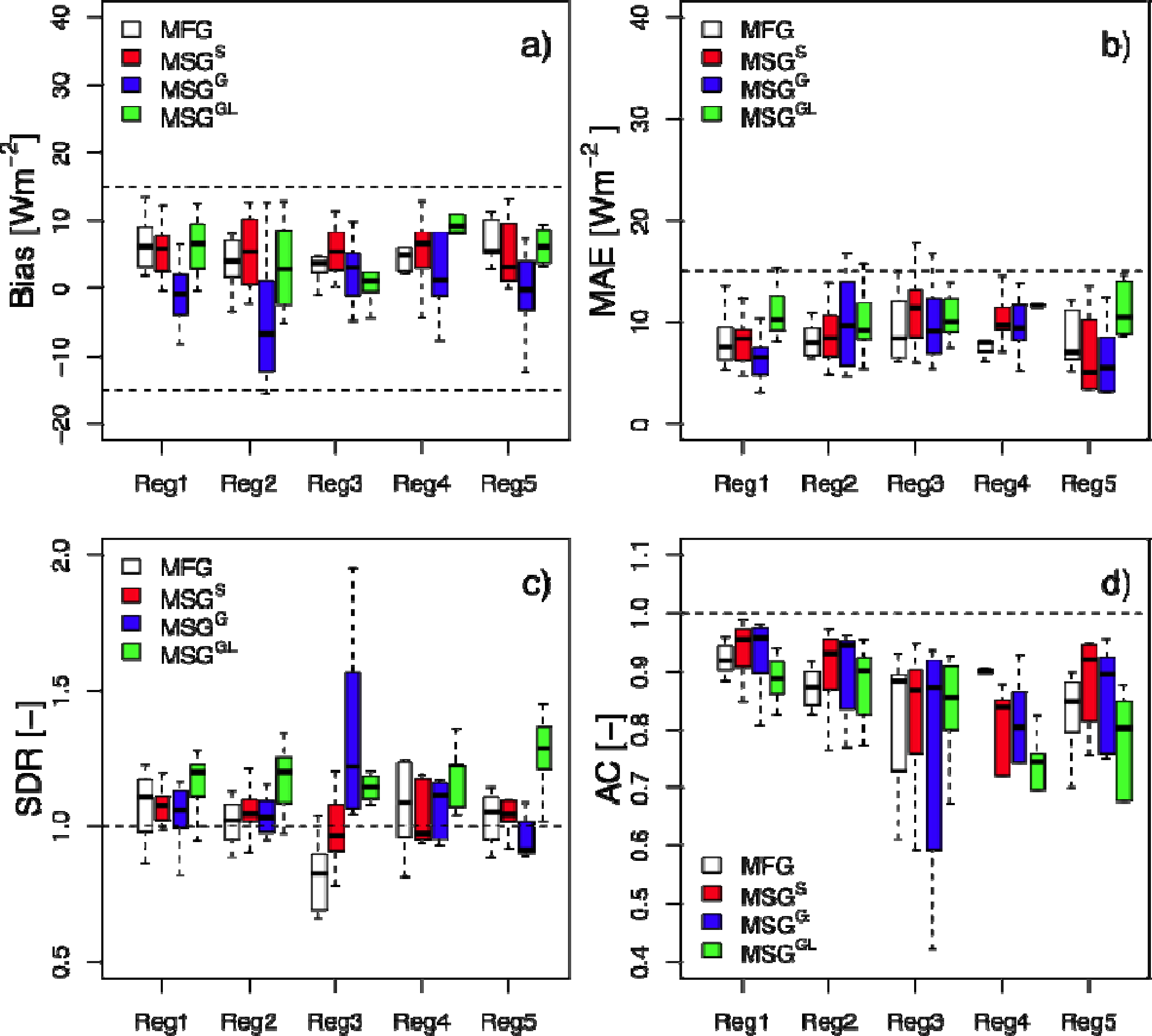
Figure 3 provides a detailed illustration of the statistics of the comparison with the GEBA stations in five regions (see Figure 1). In general, the spread of the corresponding statistics was low in the five regions for MFG. MSGS showed the highest consistency with MFG in terms of both the mean and the spread of the corresponding statistics. MSGG yielded the smallest mean bias, with values close to zero, except for region 2. However, MSGG showed considerable spread in the bias and for the remaining statistics it was slightly outperformed by MFG. In terms of the mean bias MSGGL performed similarly to MFG, except for region 4. Yet, MSGGL was outperformed by MFG and the two other MSG datasets in terms of SDR and anomaly correlation. This might be, at least partly, induced by a bug in the processing.
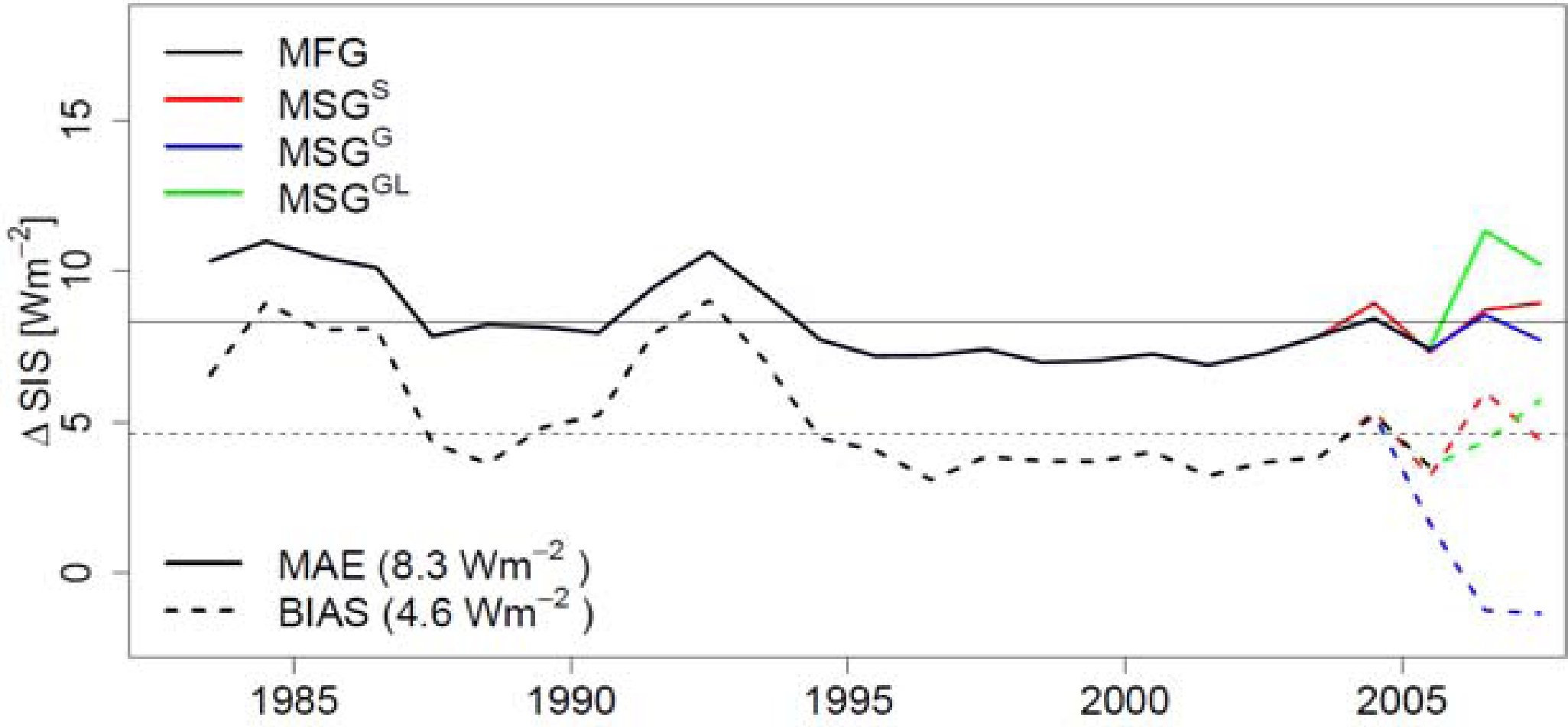
Figure 4 shows the temporal variation of mean annual bias and MAE over the period 1983–2007. Both statistics indicate inhomogeneities during the study period, particularly before 1994. The most prominent features are the two maxima around 1985 and 1992 and the reduced mean bias and MAE during the intermediate period (1987–1991) with values that are close to those obtained after 1994. The decrease in the bias and the MAE after 1987 may be related to the gain shift of the maximal reflectance in May 1987 [39]. The second maximum (1991–1994) may be related to an aerosol effect following the Pinatubo volcanic eruption in 1992. While the additional stratospheric aerosol loading reduced the SIS as observed by the surface measurements due to scattering of incident solar radiation, this effect is not considered in the satellite-derived SIS CDR (see [20]). In addition, in the period before 1994 the MVIRI data contained stripes and other artefacts that may also impact the temporal stability of the CM SAF SIS CDR before 1994.
While both MSGS and MSGG performed comparably to MFG in terms of annual mean bias, MAE, MSGG showed considerably lower annual mean bias values (but similar MAE). MSGG uses a new GADS [32]/OPAC [33] aerosol climatology, which is optically denser than the aerosol climatology used for MFG [34] and is likely to help constrain the mean SIS.
Section 4.1 and Figure 4 show that MSGS provides consistent SIS values compared to MFG and thus represents a homogeneous extension of the CM SAF SIS CDR based on MFG. However, as stated in previous works (see [19,20]) and as indicated by Figure 4, the CM SAF SIS CDR is not completely homogeneous before 1994. The lack of temporal homogeneity in the satellite-derived SIS CDR might result in incorrect conclusions and misleading results, especially if temporal changes and trends are assessed that are in the same range as the artificial inhomogeneities in the dataset [20]. Thus, correcting the inhomogeneities in the CM SAF SIS CDR will enhance its suitability for climate studies over the complete observation period. For near-real time climate monitoring of anomalies and extremes, an operational dataset is required. The latter motivates the use of MSGG to extend the CM SAF SIS CDR. Moreover MSGG shows the lowest bias, which is an advantage for the operational detection of anomalies.
In the following we assess in detail the homogeneity of the combined SIS data set based on MFG and MSGG, and present and apply a methodology to remove detected inhomogeneities in the CM SAF SIS data using surface observations.
4.2. Homogeneity
The homogeneity of the extended CM SAF SIS CDR was assessed for the period 1983–2007. Special attention was paid to the times when the satellite instruments or the retrieval algorithm changed (see Table 2).
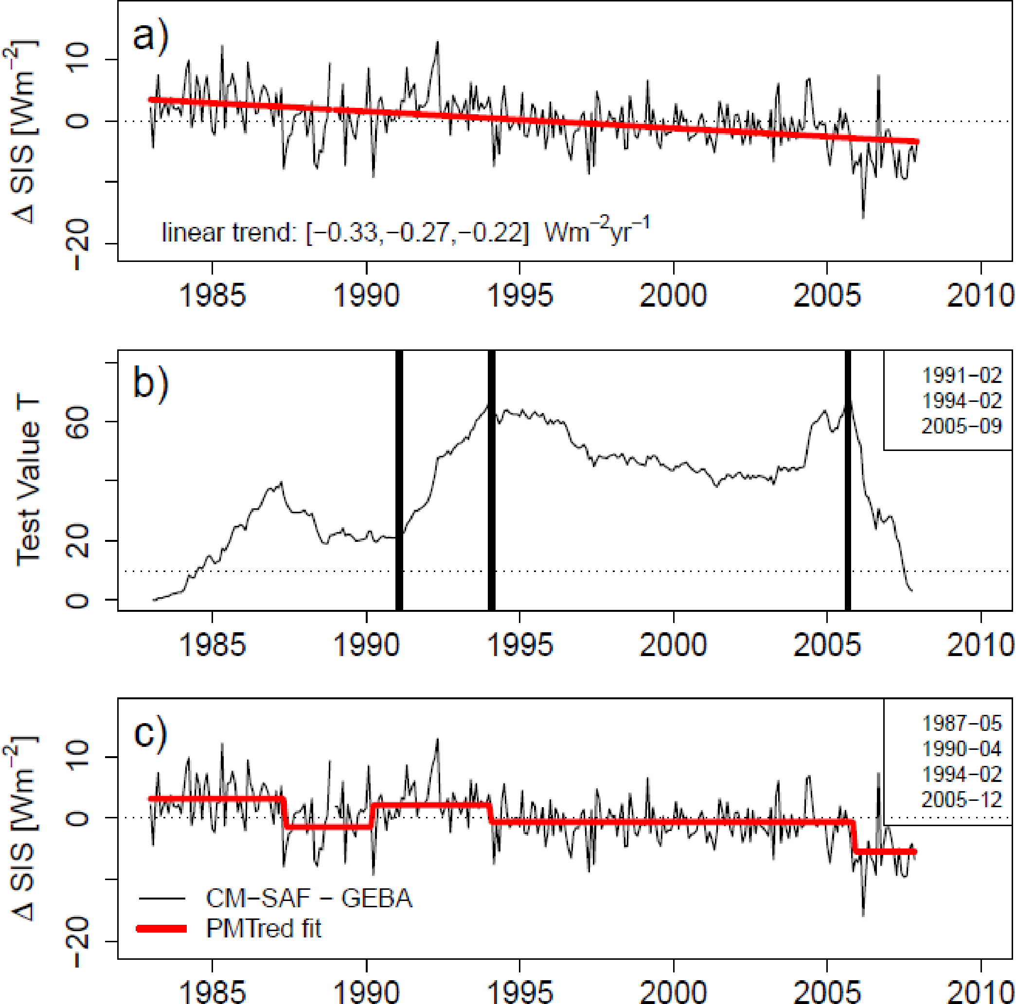
The mean difference series (CM SAF minus GEBA) of the SIS anomalies to the period 1983–2007 provided in Figure 5a shows a significant decrease of −2.7 W·m−2 per decade over the study period, suggesting that there is a lack of temporal stability in the CM SAF data as compared to the surface stations.
The result of the SNHT test is displayed in Figure 5b. The T-statistic of the SNHT test applied to the mean difference series detected major breaks (clearly significant on the 95% confidence level) in the years 1991, 1994 and 2005 (here, indicated by vertical black lines). Further possible breaks indicated by sudden changes in the slope of the T-statistic occurred in 1987, 1992, 1997 and 2003 (not shown).
Figure 5c provides the mean difference series and the PMTred fit (red line) determined using the RH test. The RH test identified several major breaks in the in the years 1987, 1990, 1994 and 2005 (the vertical offset indicates the mean shift at the breaks). Interestingly, the dates of the detected shifts agree well with the variations in the mean annual bias and MAE depicted in Figure 4.
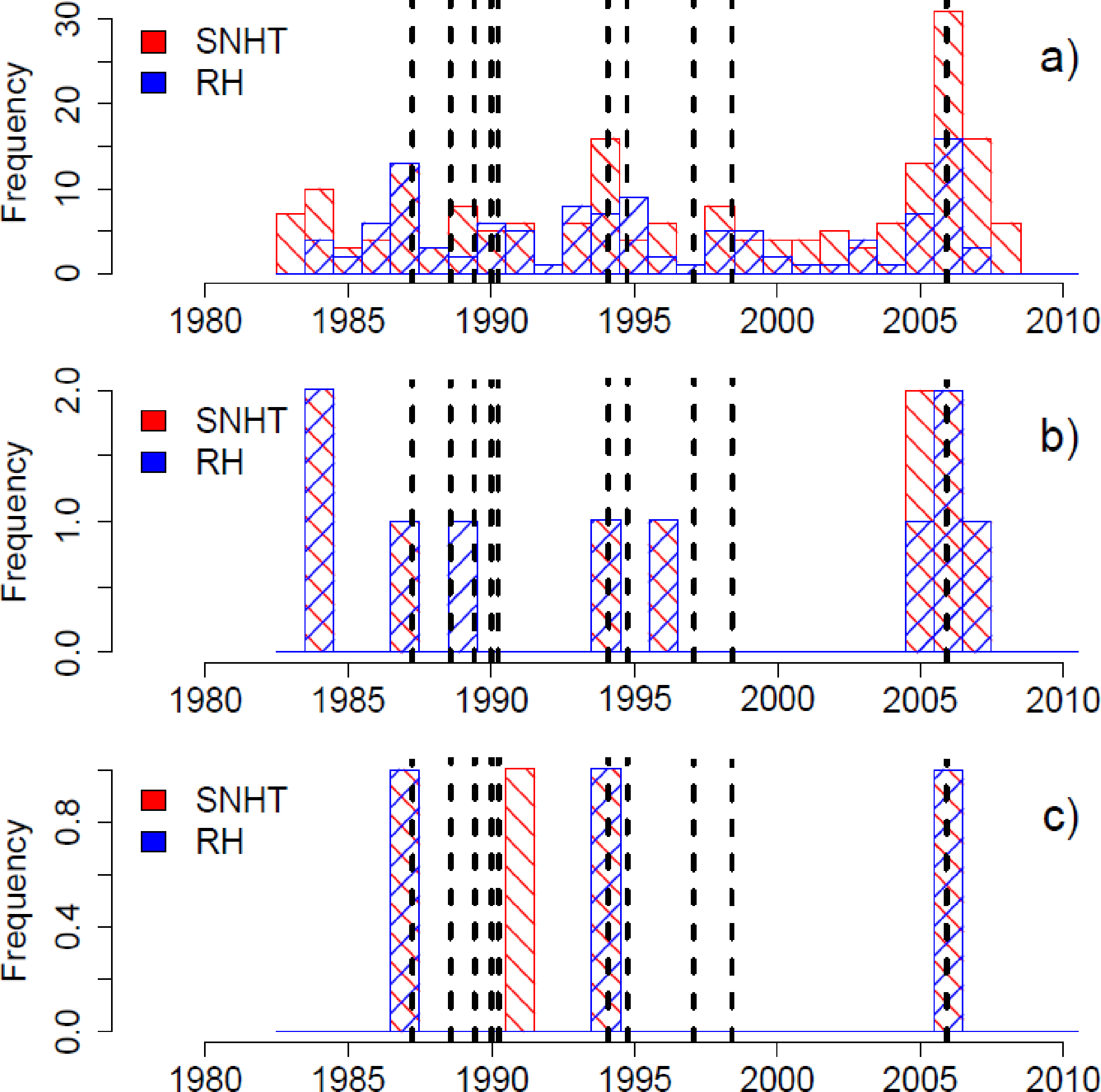
Figure 6 shows the frequency distributions of the detected shift inhomogeneities with respect to the date of their appearances using both the SNHT test (red) and the RH test (blue). The tests were applied to the series of mean monthly differences (CM SAF minus GEBA) of SIS anomalies to the period 1983–2007, for the 47 station series (panel a), regional means (panel b) and the multisite mean (panel c).
The histograms for the 47 difference series (panel a) indicate the presence of breaks associated with instrument changes (dashed lines) for a large fraction of stations. The largest impact is evidenced for the change in 2005/06, and further breaks around 1987, and 1994. Equally, both tests detected a major break in 2005/2006 for the regional mean difference series (panel b). A further break around 1984 was detected for two regional mean difference series (regions 2 and 5) that, however, could not be related to metadata information and may be due to strong anomalies (high signal-to-noise ratio) in the early observing period in the respective regions. The tests applied to the difference series of the multisite mean (Figure 6c) identified possible breaks in 1987 (only RH test), 1990 (only SNHT), 1994 and 2005/06. The four breaks (1987, 1990, 1994 and 2005/06) detected in the multisite mean series also stick out in the histograms for the individual difference series, indicating the presence of breaks on a European scale. The identified times of the breaks in the multisite mean series (1987, 1990, 1994 and 2005/06) were in good agreement with the times of change indicated in the related metadata.
4.3. Adjustment of the 47 CM SAF Series
After the identification of the significant breakpoints (times of the identified changes were modified to match the times of change indicated by metadata information), a mean-shift based adjustment was applied to the time series to remove the artificial shifts. To allow the mean-shift adjustment to vary with season, the shift sizes were determined for each calendar month separately. The performance assessment was based on a comparison with 47 GEBA stations for the period 1983–2007.
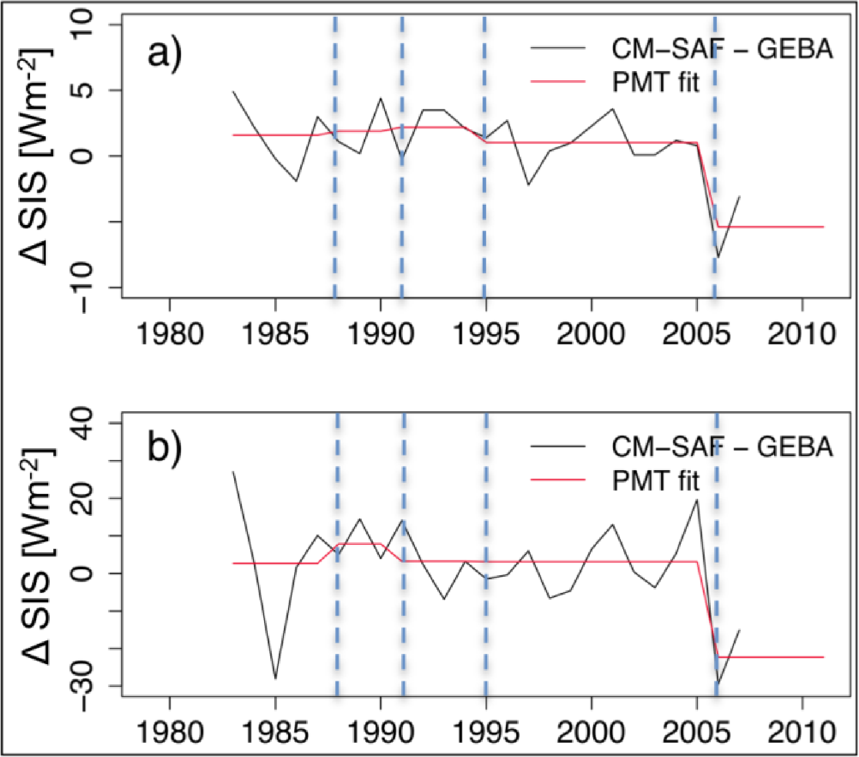
Figure 7 illustrates the shift sizes as estimated by the RH test for the January (panel a) and the July (panel b) difference series of Aberporth. Both difference series exhibited rather small shifts before 2006 and a strong shift in 2005/2006 when the MSGG dataset extends the MFG dataset. The shift sizes were stronger in the July series, which was due to the considerably higher solar radiation in summer. These results also highlight the importance of consistent satellite input data and retrieval algorithms.
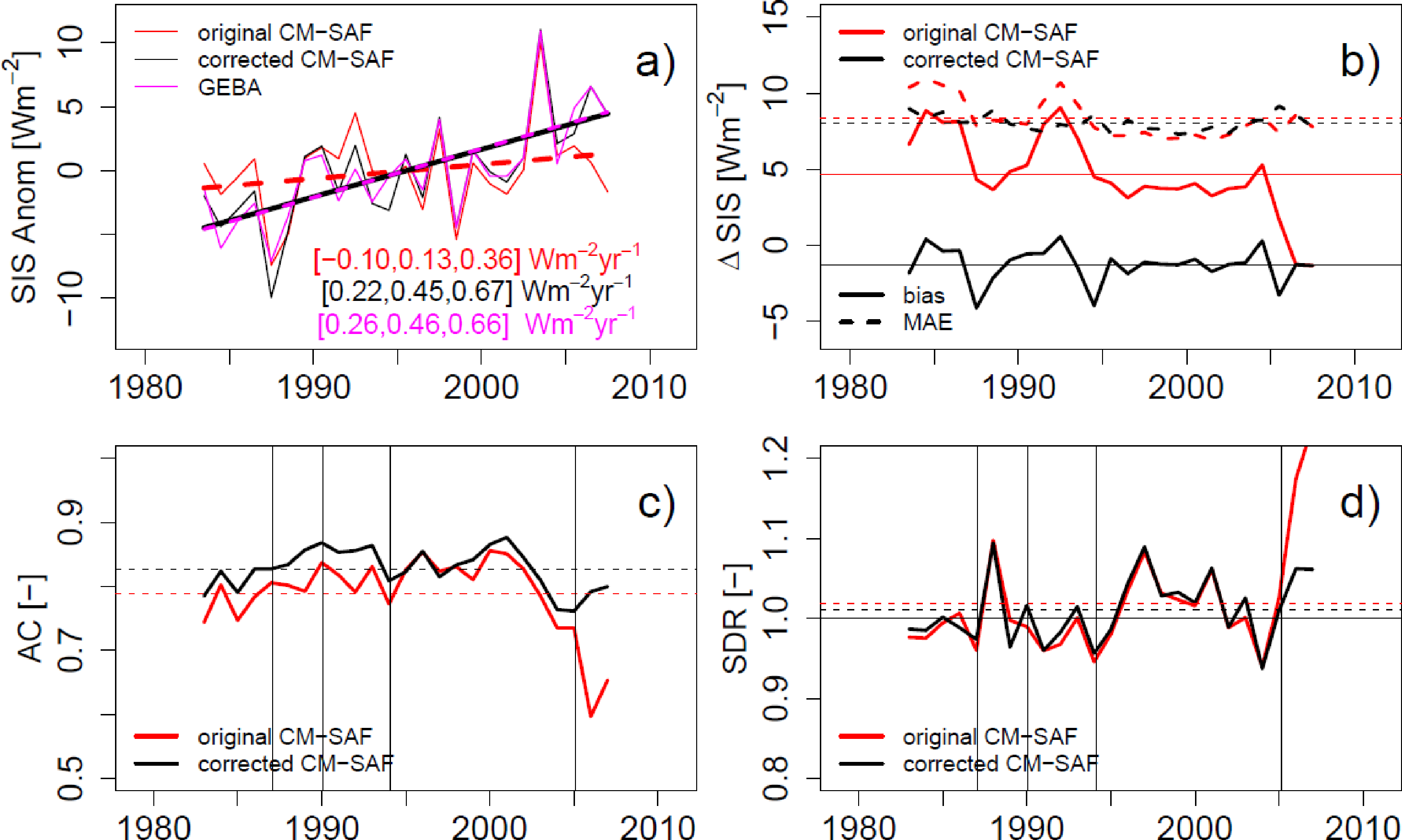
The impact of the mean-shift correction applied to the extended CM SAF series is shown in Figure 8, which depicts the temporal evolution of the mean annual anomalies (panel a), the mean annual bias and MAE (panel b), the mean annual AC (panel c) and the mean annual SDR (panel d) over the period 1983–2007.
The mean anomaly series of both the adjusted CM SAF series and the GEBA series showed very similar time evolutions and exhibited significant increases (panel a), which was also depicted by the high anomaly correlation (∼0.85) of both time series (see Table 4). While the original CM SAF series (+1.34 W·m−2 per decade) shows a considerably weaker SIS increase than the mean GEBA series (+4.59 W·m−2 per decade), the trend depicted by the corrected CM SAF series is much more consistent with the mean GEBA series (+4.47 W·m−2 per decade) over the study period.
Both the mean annual bias and the MAE of the corrected CM SAF series show a higher temporal stability over the study period compared to that of the original series (panel b). In addition, the corrected series are substantially improved over the original series in terms of mean bias (reduction from 4.65 to −1.28 W·m−2) and MAE (reduction from 8.33 to 8.00 W·m−2). Overall, the bias decreases for 79% and the MAE even for 92% of the 47 difference series (not shown).
The corrected CM SAF series show consistently higher anomaly correlations than the original series (panel c), particularly before 1994 and after 2005. The reduction in the anomaly correlation around 2004 refers to the stronger mean annual bias (see panel b) that may be due to a degradation of the MVIRI instrument on the Meteosat 7 satellite.
Panel d shows the temporal evolution of mean annual SDR of the SIS anomalies between the CM SAF series and the GEBA series (anomalies from the 1983–2007 mean). The annual mean SDR of the original CM SAF series was temporally relatively stable until 2005, however, it increased significantly after 2006. This can be explained by the overall higher SDD of the MSGG dataset (see Tables 3 and 4) due to an overall worse anomaly correlation between CM SAF and GEBA during the winter months since 2006 (Figure 8c). The mean-shift corrected CM SAF series shows no clear improvement over the original series in terms of SDR, except for the time period after 2006 when the ratio dropped from 1.3 to ∼1.
4.4. Adjustment of the CM SAF Series over the European Region
As indicated in Section 3, the grid-point-wise adjustment of the CM SAF SIS data was done using linear regression that relates the station-wise derived mean-shifts to the difference field (e.g., MSGG minus MFG, see Figure 2) in the overlap period (April to December 2005) and to the geographical coordinates.
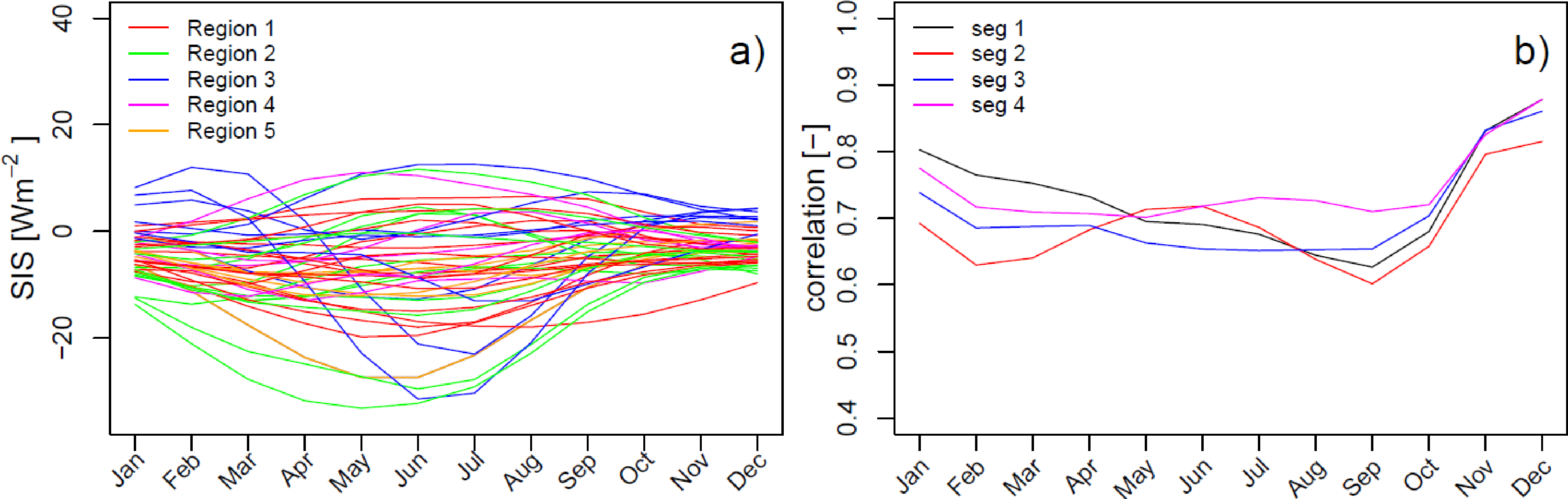
Figure 9a shows the smoothed annual cycles of the mean-shifts obtained for the 47 difference series between segment four (1994–2005) and the reference segment (2006 onwards). Figure 9b shows for each calendar month the correlations between the station-wise obtained mean-shifts at the significant breakpoints (e.g., between each segment and the last segment) and the difference field at the station locations. The station-wise derived mean-shifts depict a seasonal dependency with smaller shifts during winter and considerably larger shifts during summer (panel a). Also the pattern in the difference fields (Figure 2) of the two CM SAF datasets shows strong seasonal variations. The seasonality of the shift sizes is thereby mainly governed by the seasonally varying solar zenith angle and the land-sea distribution. A smoothing spline function with six degrees of freedom was applied to the annual cycles of both the station-wise derived mean-shifts and the difference field (not shown), to remove fluctuations in the annual cycles due to measuring uncertainties and the rather short last segment (2006–2007). The high correlations between the mean-shifts derived for the 47 difference series and the difference field shown in panel b highlight the similarity of the obtained shifts.
The performance of the correction method was assessed using cross-validation. Here, we estimated the mean-shifts using the regression-based approach (Section 3.2.1) by leaving-out each difference series once in turn. Subsequently the estimated mean-shifts were applied to correct the 47 CM SAF series. Table 5 provides the validation results for the corrected CM SAF SIS CDR (uncorrected in brackets) at the 47 GEBA series for the period 1983–2007. The biases in the corrected CM SAF series decreased substantially in all months, resulting in negative biases in autumn and winter and biases close to zero in spring and summer. The average bias decreased from 4.7 W·m−2 to −1.4 W·m−2, thus the average bias of the corrected CM SAF series corresponds with the mean bias of the operationally derived SIS since 2006 (see Table 3) and is more stable in time. The higher stability of the corrected CM SAF series was confirmed by the anomaly-based statistics. The mean anomaly correlation increased from 0.75 to 0.79, with the strongest improvement in winter. Additionally, the mean-shift correction was able to decrease the spread (SDD) and to increase the fraction of monthly data meeting the target accuracy. The higher improvement during winter (especially for AC) can be explained by the larger relative bias in the uncorrected datasets in that season.
These findings demonstrate that regression-based interpolation of the mean-shifts using the difference field as predictor properly accounts for regional differences in the shift sizes, and thus is useful to adjust the extended CM SAF dataset over the European region.
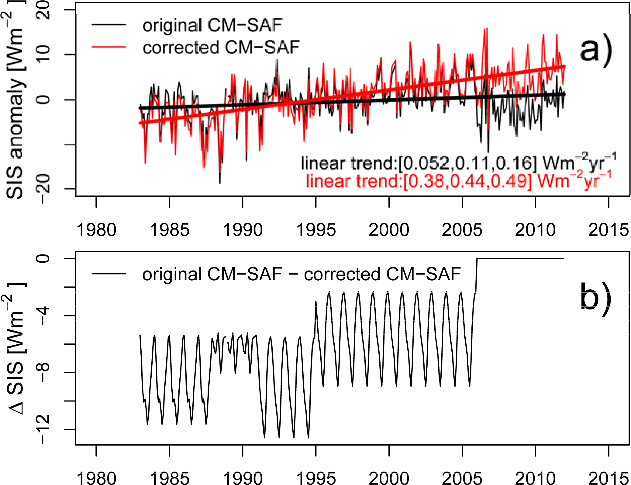
Figure 10 shows the temporal evolution of the monthly mean SIS anomaly series (relative to 1983–2007) from the original and the corrected CM SAF dataset (panel a), and the mean difference series between the original and the corrected CM SAF anomalies (panel b) over the European region (e.g., the area evaluated in Figure 10) for the period 1983–2007. Both time series (panel a) showed a very similar temporal evolution on monthly time scales with significantly positive trends, particularly from 1994 to 2005. However, the rate of increase was clearly stronger for the corrected series (+4.3 W·m−2 per decade) than for the original series (+1.1 W·m−2 per decade) over the study period. The time series of the difference between the corrected and the original CM SAF anomalies exhibited a strong seasonal cycle (panel b), due to the seasonal dependency of the mean-shifts (see Figure 9a). In general, the mean adjustment over all grid points was negative before 2006, although closer to zero in winter, resulting in an intensification of the positive trend of SIS anomalies in the corrected CM SAF series. Largest adjustments were applied in the summer months, with mean-shifts of up to 12 W·m−2. In winter the adjustments stayed within the range of −6 to −3 W·m−2.
4.5. Error Sources
In comparison to the ground-based reference, the homogenised data record shows an improvement over the original data record in terms of anomaly correlation and bias. Some undesirable but explainable effects resulted from the applied correction procedure, such as underestimated shift sizes during summer. Several reasons have been found that help to understand the draw-backs in the corrected data, including the limited number of reference stations available and uncertainties inherent in both the reference and the satellite data.
(a) Limited number of reference stations: Errors are introduced through the assumption that station-wise detected mean-shifts for any date are correlated with the differences obtained between MVIRI- and GERB-derived SIS. However, currently there are not sufficient ground-based stations available for a direct mean-shift calculation from the difference series at every grid point. We expect that all the MVIRI instruments before 2005 have similar spectral sensitivities and therefore the pattern of differences of the MVIRI instrument to the GERB instrument will be similar for all MVIRI instruments. These relationships were used to correct the satellite-based estimates at locations where ground-based reference data was unavailable.
Uncertainties accompanying the mean-shift determination were reduced by applying a smoothing spline to the annual cycle of the station-wise derived mean-shifts and the difference field. A comprehensive analysis using the mean-shift corrected time series showed a significant reduction in the bias and an increase in anomaly correlation in comparison to the GEBA reference observations.
(b) Uncertainties inherent in the observational datasets: Figure 11 shows the spatial distribution of the differences between the monthly SIS data from the original MFG and the MSGG data sets (top row) and the differences between the SIS data from the corrected MFG and the MSGG data sets (bottom row), for April, July, September and December 2005. The differences, which were particularly high during the vegetation period over North Africa, are mainly attributed to the spectral properties of the broadband channel of the MVIRI instrument and the GERB visible channel. However, also different aerosol climatologies and retrieval algorithms contribute to the observed differences between MFG and MSG based SIS.
The correction method worked particularly well over Europe in autumn and winter, reducing the overestimates in MFG from up to 40 W·m−2 in some regions to below 15 W·m−2 (Figure 11, bottom row). Also the large differences in the regions north of 60°N (Figure 10, top row) are reduced. Yet, the very strong differences between MFG and MSGG in April do not completely disappear. This can be explained by uncertainties inherent in the station-wise determined mean-shifts, due to limitations in the accuracy of the satellite and the ground-based observations and due to the short last segment (2006–2007). While the SIS observations by the ground-based GEBA stations have an estimated accuracy of about 5 W·m−2 [20], the requirement for solar surface irradiance retrieved from satellites is 10 W·m−2 [29]. As indicated in Section 3, a smoothing spline with six degrees of freedom has been applied to remove outliers in the annual cycles of the mean-shifts. As a consequence the applied mean-shifts are reduced compared to the true shift sizes (not shown). While this smoothing might be non-ideal, the application of unsmoothed mean-shifts may introduce additional uncertainties in the corrected dataset. It should be noted that this method is designed only to reduce the systematic errors, not the random errors. The latter are difficult to quantify or correct, especially when the ground reference data themselves are not error-free (e.g., [28,29]).
(c) Additional error sources: While the above mentioned limited station coverage and the uncertainties inherent in both datasets are mainly responsible for the draw-backs in the corrected data, another factor might also contribute to this. In the period before 1994 the MVIRI data contained stripes and other artefacts that may also impact the temporal stability of the CM SAF SIS CDR before 1994.
5. Summary and Conclusions
Large efforts have been made in recent years for the generation of homogeneous and consistent long-term climate data records (CDRs). While their high quality generally enables the assessment of climate variability and climate change they suffer, however, from a reduced timeliness. CDRs are generally not sustained in near-real-time but rather reprocessed with delays of several years. This reduces their usefulness in particular for near real-time climate monitoring and for the assessments of current trends or recent climate extremes. While environmental data records (EDRs) provided in near real-time compensate for this shortcoming, they suffer from reduced record length. We follow the argumentation by other authors (e.g., AghaKouchak and Nakhjiri, 2012) that practices for monitoring and analysis of essential climate variables (ECVs) should combine the advantages of CDRs (i.e., length, homogeneity) with those of EDRs (i.e., timeliness).
In this study, we propose a method to bridge the gap between long-term climate data records and near real-time data. We test this new approach for the homogenisation of satellite-based monthly mean surface incoming solar radiation (SIS) estimates provided by the EUMETSAT Satellite Application Facility on Climate Monitoring (CM SAF). A preliminary inter-comparison of three extended CM SAF SIS climate data record (CDR) versions identified the operationally generated SIS dataset (MSGG) as the most suitable to extend the CM SAF SIS CDR, due to its low bias.
The method consists of break detection using ground-based reference station observations, break visualization and finally break adjustment. Adjustments were based on the mean-shift in the difference series between the satellite dataset and the surface reference observation between any segment and the reference segment. To allow for seasonal variations in the adjustment, the mean-shifts were calculated for each calendar month separately.
There were spatially and temporally varying statistical relationships between the station-wise determined mean-shifts and the difference between Meteosat First Generation (MFG) and MSGG SIS. These relationships were used to correct the satellite-based estimates at locations where ground-based reference data was unavailable. Uncertainties accompanying the mean-shift determination were reduced by applying a smoothing spline to the annual cycle of the station-wise derived mean-shifts and the difference field. The method has been tested for the CM SAF datasets over the European region for the overlap-period when both MFG and MSGG data were available. The method worked particularly well over Europe in autumn and winter, reducing the overestimates in MFG from up to 40 W·m−2 in some regions to below 15 W·m−2. The application of the method to other regions than Europe will generally depend on the density of surface-based SIS observations.
The performance of the proposed method is encouraging for the feasibility of extending CDRs into near real-time and future research is warranted. The mean-shift corrected time series of combined CDR and EDR showed a significant reduction in the bias and an increase in anomaly correlation, providing a more homogeneous near-real-time climate data record.
We argue that the generation of climate data records in near real-time would offer unique opportunities for climate monitoring and research. Multiple applications would benefit from a near real-time SIS dataset, e.g., studies of global dimming and brightening, analysis of climate extremes (e.g., heat waves) or solar energy applications. Thus, we would be motivated for the application of the proposed method for the operational generation of near-real-time climate data records in order to facilitate a better analysis of the current state of the climate and to provide better climate services.
Although our proposed method has been developed for SIS datasets it is applicable for the adjustment of CDRs addressing other ECVs as well, provided that appropriate ground-based measurements and a priori knowledge about changes of algorithm, instrumentation or satellites are available. Nevertheless, the applicability of the method for the adjustment of satellite datasets addressing other variables needs to be assessed in future studies. Moreover, additional work is required when the method is used with other geostationary satellites to build a homogeneous global SIS climate data record.
Acknowledgments
Meteosat data were provided by EUMETSAT’s Satellite Application Facility on Climate Monitoring (CM SAF). The contribution of surface radiation data from the GEBA network kindly provided by the ETH Zurich and the various field sited to the BSRN archive and its maintenance at the AWI is greatly appreciated. S.K. and B.A. acknowledge funding from the Deutscher Wetterdienst (DWD), Offenbach and from the Hessian initiative for development of scientific and economic excellence (LOEWE) at the Biodiversity and Climate Research Centre (BiK-F), Frankfurt/Main. We also thank the three reviewers for their constructive comments and helpful suggestions on the manuscript.
Conflicts of Interest
The authors declare no conflict of interest.
References
- SCOPE-CM. Implementation Plan for the Sustained and Coordinated Processing of Environmental Satellite Data for Climate Monitoring (SCOPE-CM), Version 1.3; SCOPE-CM Report; Geneva, Switzerland, 2009. [Google Scholar]
- Lattanzio, A.; Schulz, J.; Matthews, J.; Okuyama, A.; Theodore, B.; Bates, J.J.; Knapp, K.R.; Kosaka, Y.; Schüller, L. Land Surface Albedo from Geostationary Satelites: A Multiagency Collaboration within SCOPE-CM. Bull. Amer. Meteorol. Soc 2013, 94, 205–214. [Google Scholar]
- Ohring, G.; Wielicki, B.A.; Spencer, R.; Emery, B.; Datla, R. Satellite instrument calibration for measuring global climate change: Report of a workshop. Bull. Am. Meteorol. Soc 2005, 86, 1303–1313. [Google Scholar]
- Schulz, J.; Albert, P.; Behr, H.-D.; Caprion, D.; Deneke, H.; Dewitte, S.; Dürr, B.; Fuchs, P.; Gratzki, A.; Hechler, P.; et al. Operational climate monitoring from space: the EUMETSAAT Satellite Application Facility on Climate Monitoring (CM-SAF). Atmos. Chem. Phys 2009, 9, 1687–1709. [Google Scholar]
- Trenberth, K. E.; Anthes, R. A.; Belward, A.; Brown, O.; Haberman, E.; Karl, T. R.; Running, S.; Ryan, B.; Tanner, M.; Wielicki, B. Challenges of a Sustained Climate Observing System. In Climate Science for Serving Society: Research, Modelling and Prediction Priorities; Hurrell, J.W., Asrar, G., Eds.; Springer: Berlin, Germany, 2013. [Google Scholar]
- AghaKouchak, A.; Nakhjiri, N. A near real-time satellite-based global drought climate data record. Environ. Res. Lett 2012, 7, 044037. [Google Scholar]
- Tian, Y.; Peters-Lidard, C.D.; Eylander, J.B. Real-time bias reduction for satellite-based precipitation estimates. J. Hydrometeorol 2010, 11, 1275–1285. [Google Scholar]
- Liu, Y.Y.; Dorigo, W.A.; Parinussa, R.M.; de Jeu, R.A.M.; Wagner, W.; McCabe, M.F.; Evans, J.P.; van Dijk, A.I.J.M. Trend-preserving blending of passive and active microwave soil moisture retrievals. Remote Sens. Environ 2012, 123, 280–297. [Google Scholar]
- Comiso, J.C.; Nishio, F. Trends in the Sea Ice Cover Using Enhanced and Compatible AMSR-E, SSM/I, and SMMR Data. J. Geophys. Res. 2008, 113. [Google Scholar] [CrossRef]
- Huld, T.; Müller, R.; Gambardella, A. A new solar radiation database for estimating PV performance in Europe and Africa. Solar Energy 2012, 86, 1803–1815. [Google Scholar]
- Kothe, S.; Dobler, A.; Beck, A.; Ahrens, B. The radiation budget in a regional climate model. Clim. Dyn 2011, 36, 1023–1036. [Google Scholar]
- Dobler, A.; Müller, R.; Ahrens, B. Development and evaluation of a simple method to estimate evaportation from satellite data. Meteorol. Z 2011, 20, 615–623. [Google Scholar]
- WMO Regional Climate Centre on Climate Monitoring for Europe and the Middle East. Available online: www.dwd.de/rcc-cm(accessed on 17 September 2013).
- Posselt, R.; Mueller, R.; Trentmann, J. Spatial and temporal homogeneity of solar surface irradiance across satellite generations. Remote Sens 2011, 3, 1029–1046. [Google Scholar]
- 23-year long CDR of surface solar radiation parameters including solar surface irradiance (SIS) and direct irradiance (SID) for the period 1983–2005. Available online: www.cmsaf.eu (accessed on 17 September 2013). [CrossRef]
- Rossow, W.; Dueñas, E. The international satellite cloud climatology project (ISCCP) web site: An online resource for research. Bull. Am. Meteorol. Soc 2004, 85, 167–172. [Google Scholar]
- Gupta, S.; Stackhouse, P., Jr.; Cox, S.; Mikovitz, J.; Zhang, T. Surface radiation budget project completes 22-year data set. GEWEX News 2006, 16, 12–13. [Google Scholar]
- Berrisford, P.; Dee, D.; Fielding, K.; Fuentes, M.; Kallberg, P.; Kobayashi, S.; Uppala, S. The ERA-Interim Archive. In ERA Report Series; ECMWF: Shinfield Park: Reading, UK, 2009; pp. 16–17. [Google Scholar]
- Brinckmann, S.; Trentmann, J.; Ahrens, B. Homogeneity analysis of the CM SAF solar surface irradiance data set derived from geostationary satellite observations. Remote Sens. 2013. submitted.. [Google Scholar]
- Sanchez-Lorenzo, A.; Wild, M.; Trentmann, J. Validation of the means and temporal stability in the CM SAF high-resolution surface solar radiation product over Europe against a homogenized surface dataset (1983–2005). Remote Sens. Environ 2013, 134, 355–366. [Google Scholar]
- Alexandersson, H.; Moberg, A. Homogenization of Swedish temperature data. Part I: Homogeneity test for linear trends. Int. J. Climatol 1997, 17, 25–34. [Google Scholar]
- Wang, X. Accounting for autocorrelation in detecting mean shifts in climate data series using the penalised maximal t or F test. J. Appl. Meteor. Climatol 2008, 47, 2423–2444. [Google Scholar]
- Wang, X. Penalized maximal F test for detecting undocumented mean shift without trend change. J. Atmos. Oceanic Technol 2008, 25, 368–384. [Google Scholar]
- Wild, M. Global dimming and brightening: A review. J. Geophys. Res. 2009, 114. [Google Scholar] [CrossRef]
- Cano, D.; Monget, J.M.; Albuisson, M.; Guillard, H.; Regas, N.; Wald, L. A method for the determination of the global solar-radiation from meteorological satellite data. Solar Energy 1986, 37, 31–39. [Google Scholar]
- Beyer, H.G.; Costanzo, C.; Heinemann, D. Modifications of the heliosat procedure for irradiance estimates from satellite images. Solar Energy 1996, 56, 207–212. [Google Scholar]
- Mueller, R.; Matsoukas, C.; Gratzki, A.; Behr, H.; Hollmann, R. The CM-SAF operational scheme for the satellite based retrieval of solar surface irradiance—A LUT based eigenvector hybrid approach. Remote Sens. Environ 2009, 113, 1012–1024. [Google Scholar]
- Mueller, R.; Trentmann, J.; Träger-Chatterjee, C.; Posselt, R.; Stöckli, R. The role of the effective cloud albedo for climate monitoring and analysis. Remote Sens 2011, 3, 2305–2320. [Google Scholar]
- Posselt, R.; Mueller, R.; Stöckli, R; Trentmann, J. Remote sensing of solar radiation for climate monitoring—The CM-SAF retrieval in international comparison. Remote Sens. of Environ 2012, 188, 186–198. [Google Scholar]
- Posselt, R.; Mueller, R.; Trentmann, J.; Stöckli, R.; Liniger, M. A surface radiation climatology across two Meteosat satellite generations. J. Geophys. Res 2013, 15. EGU2013-7129. [Google Scholar]
- Cros, S.; Albuisson, M.; Wald, L. Simulating Meteosat-7 broadband radiances using two visible channels of Meteosat-8. Solar Energy 2006, 80, 361–367. [Google Scholar]
- Koepke, P.; Hess, M.; Schult, I.; Shettle, E.P. Global Aerosol Dataset; Report N 243; Max-Plank-Institut für Meteorologie: Hamburg, German, 1997; p. 44. [Google Scholar]
- Hess, M.; Koepke, P.; Schult, I. Optical Properties of Aerosols and Clouds: The software package OPAC. Bull. Amer. Meteorol. Soc 1998, 79, 831–844. [Google Scholar]
- Kinne, S.; O’Donnel, D.; Stier, P.; Kloster, S.; Zhang, K.; Schmidt, H.; Rast, S.; Giorgetta, M.; Eck, T.; Stevens, B. A new global aerosol climatology for climate studies. J. Adv. Model. Earth Syst. 2013. [Google Scholar] [CrossRef]
- Ohmura, A.; Gilgen, H.; Hegener, H.; Müller, G.; Wild, M.; Dutton, E.G.; Forgan, B.; Fröhlich, C.; Philipona, R.; Heimo, A.; et al. Baseline Surface Radiation Network (BSRN/WCRP): New precision radiometry for climate research. Bull. Am. Meteorol. Soc 1998, 79, 2115–2136. [Google Scholar]
- Gilgen, H.; Wild, M.; Ohmura, A. Means and trends of shortwave irradiance at the surface estimated from GEBA. J. Clim 1998, 11, 2042–2061. [Google Scholar]
- Aguilar, E.; Auer, I.; Brunet, M.; Peterson, T.C.; Wierina, J. Guidelines on Climate Metadata and Homogenization; WMO-TD No. 1186; World Meteorological Organisation: Geneva, Switzerland, 2003; p. 52. [Google Scholar]
- Rigollier, C.; Lefevre, M.; Blanc, P.; Wald, L. The operational calibration of images taken in the visible channel of the meteosat series of satellites. J. Atmos. Oceanic Technol 2002, 19, 1285–1293. [Google Scholar]
- Posselt, R. MeteoSwiss, Personal Communication,. 2012.
Appendix: Statistics Used to Evaluate the CM SIS CDR
The bias is the average difference between two datasets over n time steps. It depicts whether the considered dataset, on average, over- or under-estimates the reference dataset:
The mean absolute error (MAE) measures the deviation from the reference dataset, and is based on absolute values.
The standard deviation of the differences (SDD) measures the spread around the mean value of the distribution formed by the differences between two time series.
The anomaly correlation (AC) depicts the correlation between the anomalies of two time series without consideration of the influence of the bias.
The standard deviation ratio (SDR) describes to which extent the standard deviations of the anomalies of the two considered time series correspond to each other ignoring the influence of a possibly existing bias.
The annual cycle ȳ and ō were determined separately for each station of the satellite and the reference dataset. The monthly anomalies were then calculated by subtracting the corresponding annual cycle.
The fraction of values above the accuracy threshold (Frac) is calculated as following


| SIS Dataset | Cloudy Sky Method | Clear Sky Method | Satellite Images | Aerosols |
|---|---|---|---|---|
| MFG 1983–2005 | Heliosat method [25,26] modified with self-calibration [28] and fuzzy logic approach for clear sky reflection [14,29] | MAGIC [27] | MFG MVIRI HRV visible channel | MPI Hamburg/Kinne [34] |
| MSGS 2005–2011 | Identical to SIS MFG | MAGIC [27] | VHRV: Virtual HRV broadband channel derived from SEVIRI VIS006 and VIS008 channels [31] | MPI Hamburg/Kinne [34] |
| MSGG operational 2006–today | MAGIC [27] | MAGIC [27] | MSG GERB visible broadband measurements, spatial down-scaling with SEVIRI data | GADS [30]/OPAC [33] aerosols |
| MSGGL 2006–2011 | Identical to SIS MFG but with classical minima approach for clear sky reflection instead of fuzzy logic. | MAGIC [27] | MSG GERB-like data: VIS broadband data calculated from SEVIRI and adjusted to GERB. | MPI Hamburg/Kinne [34] |
| Event | Date |
|---|---|
| Meteosat 2 | 16.8.1981–11.8.1988 |
| Gain shift | May 1987 (Rebekka Posselt, pers.com.) |
| Meteosat 3 | 11.8.1988–19.6.1989 |
| Meteosat 4 | 19.6.1989–24.1.1990 |
| Meteosat 3 | 24.1.1990–19.4.1990 |
| Meteosat 4 | 19.4.1990–4.2.1994 |
| Meteosat 5 | 4.2.1994–13.2.1997 |
| Meteosat 6 | 13.2.1997–3.6.1998 |
| Meteosat 7 | 3.6.1998–31.12.2005 |
| Meteosat 8 | 31.12.2005–11.4.2007 |
| Meteosat 9 | 11.4.2007–21.1.2013 |
| SIS (Monthly Mean) | nmon | Bias [W·m−2] | MAE [W·m−2] | SDD [W·m−2] | AC | Fracmon [%] Bias > 15 W·m−2 |
|---|---|---|---|---|---|---|
| 1990–2005 (MFG) | 377 | 7.2 | 8.1 | 6.0 | 0.84 | 11.4 |
| 2001–2005 (MFG) | 205 | 7.0 | 7.9 | 5.7 | 0.83 | 8.3 |
| 2006–2009 (MSGS) | 184 | 7.9 | 8.7 | 7.1 | 0.87 | 13.6 |
| 2006–2010 (MSGG) | 221 | −3.7 | 7.4 | 8.0 | 0.83 | 12.7 |
| 2006–2010 (MSGGL) | 227 | 5.7 | 9.2 | 8.5 | 0.81 | 18.1 |
| SIS (Monthly Mean) | nmon | Bias [W·m−2] | MAE [W·m−2] | SDD [W·m−2] | AC | Fracmon [%] Bias > 15 W·m−2 |
|---|---|---|---|---|---|---|
| 1983–2005 (MFG) | 12,925 | 5.23 | 8.86 | 6.7 | 0.87 | 15.6 |
| 2004–2005 (MFG) | 1,128 | 4.4 | 9.25 | 8.7 | 0.84 | 13.2 |
| 2006–2007 (MSGS) | 1,075 | 5.25 | 9.88 | 5.3 | 0.88 | 18 |
| 2006–2007 (MSGG) | 1,114 | −1.28 | 8.68 | 11.2 | 0.87 | 14.9 |
| 2006–2007 (MSGGL) | 1,080 | 5.06 | 10.02 | 8.8 | 0.83 | 25 |
| Mon | n | BIAS | MAE | SDD | AC | Frac [%] > 15 W·m−2 | SDR |
|---|---|---|---|---|---|---|---|
| Jan | 1,175 | −2.8 [2.1] | 4.6 [4.5] | 3.9 [4.3] | 0.60 [0.53] | 3 [1] | 1.08 [1.10] |
| Feb | 1,175 | −4.7 [1.5] | 7.4 [6.8] | 6.5 [6.8] | 0.68 [0.68] | 12 [8] | 1.08 [1.13] |
| Mar | 1,175 | −2.5 [5.1] | 9.0 [10.4] | 8.3 [9.3] | 0.82 [0.77] | 19 [24] | 1.05 [1.02] |
| Apr | 1,175 | 0.3 [8.2] | 10.0 [12.2] | 9.3 [10.3] | 0.87 [0.83] | 22 [33] | 1.07 [1.00] |
| May | 1,175 | −0.5 [7.1] | 11.8 [11.2] | 10.3 [10.8] | 0.89 [0.88] | 30 [27] | 1.06 [1.05] |
| Jun | 1,175 | −0.7 [6.7] | 11.5 [11.6] | 10.4 [11.0] | 0.89 [0.88] | 27 [26] | 1.04 [1.02] |
| Jul | 1,175 | 0.6 [7.7] | 10.5 [11.4] | 9.9 [10.6] | 0.90 [0.88] | 25 [27] | 0.97 [0.97] |
| Aug | 1,150 | 0.6 [6.7] | 9.1 [10.0] | 8.5 [9.1] | 0.89 [0.88] | 18 [21] | 1.10 [1.13] |
| Sep | 1,175 | −1.5 [3.1] | 6.9 [6.7] | 7.2 [7.4] | 0.88 [0.87] | 10 [9] | 1.04 [1.02] |
| Oct | 1,175 | −2.7 [1.6] | 5.4 [5.5] | 5.2 [5.9] | 0.84 [0.80] | 4 [4] | 1.08 [1.10] |
| Nov | 1,172 | −0.4 [3.8] | 4.2 [5.8] | 4.6 [5.5] | 0.64 [0.58] | 2 [5] | 1.15 [1.27] |
| Dec | 1,073 | −2.2 [2.2] | 3.5 [3.9] | 3.1 [3.7] | 0.58 [0.46] | 1 [0] | 1.04 [1.16] |
| Annual | 13,995 | −1.4 [4.7] | 7.9 [8.3] | 7.3 [7.9] | 0.79 [0.75] | 15 [16] | 1.06 [1.08] |
© 2013 by the authors; licensee MDPI, Basel, Switzerland This article is an open access article distributed under the terms and conditions of the Creative Commons Attribution license ( http://creativecommons.org/licenses/by/3.0/).
Share and Cite
Krähenmann, S.; Obregon, A.; Müller, R.; Trentmann, J.; Ahrens, B. A Satellite-Based Surface Radiation Climatology Derived by Combining Climate Data Records and Near-Real-Time Data. Remote Sens. 2013, 5, 4693-4718. https://doi.org/10.3390/rs5094693
Krähenmann S, Obregon A, Müller R, Trentmann J, Ahrens B. A Satellite-Based Surface Radiation Climatology Derived by Combining Climate Data Records and Near-Real-Time Data. Remote Sensing. 2013; 5(9):4693-4718. https://doi.org/10.3390/rs5094693
Chicago/Turabian StyleKrähenmann, Stefan, Andre Obregon, Richard Müller, Jörg Trentmann, and Bodo Ahrens. 2013. "A Satellite-Based Surface Radiation Climatology Derived by Combining Climate Data Records and Near-Real-Time Data" Remote Sensing 5, no. 9: 4693-4718. https://doi.org/10.3390/rs5094693