A Comparative Study of Three Land Surface Broadband Emissivity Datasets from Satellite Data

Abstract

This study compared three broadband emissivity (BBE) datasets from satellite observations. The first is a new global land surface BBE dataset known as the Global Land Surface Satellite (GLASS) BBE. The other two are the North American ASTER Land Surface Emissivity Database (NAALSED) BBE and University of Wisconsin Global Infrared Land Surface Emissivity Database (UWIREMIS) BBE, which were derived from two independent narrowband emissivity products. Firstly, NAALSED BBE was taken as the reference to evaluate the GLASS BBE and UWIREMIS BBE. The GLASS BBE was more close to NAALSED BBE with a bias and root mean square error (RMSE) of −0.001 and 0.007 for the summer season, −0.001 and 0.008 for the winter season, respectively. Then, the spatial distribution and seasonal pattern of global GLASS BBE and UWIREMIS BBE for six dominant land cover types were compared. The BBE difference between vegetated areas and non-vegetated areas can be easily seen from two BBEs. The seasonal variation of GLASS BBE was more reasonable than that of UWIREMIS BBE. Finally, the time series were calculated from GLASS BBE and UWIREMIS BBE using the data from 2003 through 2010. The periodic variations of GLASS BBE were stronger than those of UWIREMIS BBE. The long time series high quality GLASS BBE can be incorporated in land surface models for improving their simulation results.

1. Introduction

Land surface broadband emissivity (BBE) is a key parameter in the estimation of surface energy budget and is a common input required for a variety of radiative transfer models [1–8]. Because of limited temporal and spectral information on land surface emissivity, a constant BBE assumption or simple parameterization schemes are adopted in land surface models and climate models [9–11]. Satellite remote sensing is the only means for providing global land surface BBE with certain spatial-temporal resolutions. Furthermore, the satellite-derived realistic BBE has demonstrated its capability in improving the simulation results of global climate models [10,12].

Several BBE datasets have been produced from remote sensing data by using different methods. For example, Wilber et al., produced a global BBE (5–100 μm) with 10′ × 10′ spatial resolution for satellite retrievals of longwave radiation by assigning constant emissivity values to International Geosphere-Biosphere Program (IGBP) land cover types [13]; Ogawa et al., mapped the global monthly BBE (8–13.5 μm) by converting the Moderate-resolution Imaging Spectroradiometer (MODIS) narrowband emissivity product (approximately 5 km) and a North African BBE (8–13.5 μm) using the Advanced Spaceborne Thermal Emission and Reflectance Radiometer (ASTER) narrowband emissivity product (90 m) [14,15]. Peres et al., produced a global BBE (3–14 μm) map at a 3 km spatial resolution by converting the narrowband emissivities retrieved from the Spinning Enhanced Visible and Infrared Imager (SEVIRI) onboard METEOSAT Second Generation (MSG) using Vegetation Cover Method (VCM) [16].

Recently, some researchers have produced a few narrowband emissivity products from which the BBE could be obtained by converting it to BBE via a linear regression function [17,18], including the North American ASTER Land Surface Emissivity Database (NAALSED) composited from the ASTER narrowband emissivity product [19], the University of Wisconsin Global Infrared Land Surface Emissivity Database (UWIREMIS) retrieved by adjusting MODIS narrowband emissivity product (MOD11) with the proposed baseline fit method [20], and those derived from hyperspectral resolution thermal infrared (TIR) data [2,21–24].

These BBE and narrowband emissivity products share at least two common characteristics: (1) either the spatial or temporal resolutions of these products are limited. A few are just a BBE map at global or regional scales. There are two narrowband emissivities (summer season and winter season) in the NAALSED for the entire nine years (2000–2008). The spatial resolution of MOD11 emissivity product is 0.05°, and the spatial resolution of single nadir view of current hyperspectral resolution TIR sensors is larger than 10 km [25]. (2) Most of them are not well validated. For example, the BBE derived from ASTER, MODIS and SEVIRI narrowband emissivity are not validated [15,26]. Long time series of high spatial-temporal global land surface BBE will benefit the studies of surface energy budget. Cheng et al., [27,28] proposed the algorithms for retrieving global land surface BBE from the Advanced Very High-Resolution Radiometer (AVHRR) and MODIS optical data, and produced the global eight-day 1 km and 0.05° land surface BBE from 1981 through 2010. This product was known as the Global Land Surface Satellite (GLASS) BBE and released to public in November 2012 [29], and can be ordered from the BNU Center for Global Change Data Processing and Analysis ( http://www.bnu-datacenter.com) and Global Land Cover Facility ( http://glcf.umd.edu). GLASS emissivity has been validated by limited ground measurements obtained from several field experiments [30], and also by comparison with the BBE derived from the ASTER and MODIS narrowband emissivity products at regional scales. The objective of this study is to compare GLASS BBE, the BBE calculated from NAALSED emissivity and UWIREMIS emissivity at both the global and regional scales, and to provide a guideline for the potential users. The rest of this paper is arranged as follows. Section 2 introduces the used datasets; Section 3 describes the method of comparing three BBE datasets; the results and discussion are presented in Section 4; a brief conclusion is provided in Section 5.

2. Data

2.1. GLASS BBE

The Global Land Surface Satellite (GLASS) BBE is a BBE (8–13.5 μm) product that was derived from AVHRR and MODIS optical data with our newly developed algorithms [27,28,31,32]. GLASS BBE was composed of two parts: the first is the global eight-day 1 km land surface BBE retrieved from MODIS seven black-sky albedos ranging from 2000 through 2010; and the second is the global eight-day 0.05° land surface BBE retrieved from the AVHRR visible and near infrared (VNIR) reflectance during 1981–1999. In the algorithm used to generate GLASS BBE from MODIS albedos, the land surface was classified by five types: water, snow/ice, bare soils, vegetated areas and transition zones. Water and snow/ice were determined by the flag in the input data. The latter three types were determined by the Normalized Difference Vegetation Index (NDVI) threshold values, i.e., bare soils (0 < NDVI ≤ 0.156), vegetated areas (NDVI > 0.156), and transition zones (0.1 < NDVI < 0.2). Note there are overlapped areas between bare soils and transition zones, transition zones and vegetated areas. The BBE of water and snow/ice was assigned as 0.985 by combining BBE calculated from the emissivity spectrum in the spectral library (the ASTER spectral library [33] ( http://spclib.jpl.nasa.gov) and the MODIS UCSB spectral library ( http://www.icess.ucsb.edu/modis/EMIS/html/em.html)) and BBE calculated from the emissivity spectra simulated by radiative transfer models [34]. The BBE of bare soils, vegetated areas and transition zones were formulated as the linear function of seven MODIS narrowband black-sky albedos individually. When the NDVI was less than 0.1 or larger than 0.2, we used the formula for bare soils or vegetated areas to calculate their BBE respectively. In the overlapped areas between bare soils and transition zones (0.1 < NDVI ≤ 0.156), BBE was the average of those calculated by the formulae for bare soils and transition zones, whereas BBE for overlapped areas for transition zones and vegetated areas (0.156 < NDVI < 0.2) was the average of those calculated by the formulae for transition zones and vegetated areas. The BBE derived from the MODIS albedos was validated by the field measurements conducted over desert areas in the United States and China, and the absolute difference was found to be 0.02 [27,30]. The method of estimating BBE from AVHRR VNIR reflectance data was similar to that used for MODIS optical data. The differences lies in (1) the threshold values for identifying three land surface types. A pixel with 0 < NDVI ≤ 0.2 was identified as bare soils, a pixel with 0.145 < NDVI ≤ 0.243 was identified as transition zones and a pixel with NDVI > 0.2 was identified as vegetated areas. (2) The input of the algorithms. The inputs of the algorithm developed for AVHRR was the reflectance of Channels 1 and 2, whereas the input for the algorithm designed for MODIS was seven narrowband black-sky albedos. The BBE derived from the AVHRR was consistent with that derived from MODIS data. Comparing the BBE derived from AVHRR and MODIS data in 2000, the mean bias and RMS of the difference were 0.001 and 0.01, respectively [28].

2.2. NAALSED Emissivity

The North American ASTER Land Surface Emissivity Database (NAALSED) is a mean seasonal gridded 100 m emissivity database that composed from ASTER 90 m standard land surface temperature and emissivity (LST&E) products over North America [19]. NAALSED includes two seasons, the summer season (July–September) and winter season (Jane–March). In the generation of NAALSED, the cloud contaminated ASTER pixels are screened out [35]. For each location, NAALSED emissivity is the average emissivity of all-clear sky pixels from all the ASTER scenes acquired in the summer and winter seasons of 2000–2008. NAALSED also produced the gridded emissivity products on spatial resolutions of 1 km, 5 km and 50 km by aggregating 100 m emissivity product. NAALSED V2.0 product consists of 18 bands; the mean and standard deviation for the five bands surface narrowband emissivity, surface temperature, NDVI, a land-water map, the total yield (number of ASTER observations collected at each pixel), and geodetic latitude and longitude. NAALSED was validated by the laboratory-measured sand emissivity collected at nine pseudo-invariant sand sites in the western United States [36]. The mean difference for all nine sites and all five ASTER thermal-infrared (TIR) channels was found to be 0.016, which represents approximately a 1 K error in LST retrieval.

2.3. UWIREMIS Emissivity

The University of Wisconsin Global Infrared Land Surface Emissivity Database (UWIREMIS) is a monthly data set derived from the MODIS composited monthly 0.05° narrowband emissivity product (MODIS level 3 operational land surface emissivity product MYD11) by the baseline fit (BF) method [19]. The BF method derived global land surface emissivity at ten hinge points (3.6, 4.3, 5.0, 5.8, 7.6, 8.3, 9.3 10.8, 12.1 and 14.3 μm) by adjusting a baseline emissivity spectrum based on MOD11 land surface narrowband emissivity product according to a conceptual model of land surface emissivity. Testing by the 123 emissivity spectra in the MODIS UCSB emissivity library indicated that the BF-derived emissivity generally agrees well with the laboratory-measured emissivity in shape and magnitude. The UWIREMIS emissivity could be interpolated between the hinge points and also could be used to derive a high spectral resolution emissivity spectrum by virtue of the principal component regression and eigenvector from laboratory-measured emissivity spectra.

3. Methodology

3.1. Broadband Emissivity Calculation

The hemispherical emissivity is defined as follows [36],

$$\epsilon (h,\hspace{0.17em}\lambda )=2\pi {\int }_0^1\epsilon (\mu ,\hspace{0.17em}\lambda )\mu d\hspace{0.17em}\mu$$

(1)

where μ is the cosine of view angle, λ is the wavelength, and ε(μ, λ) is the directional emissivity. The broadband emissivity can be represented as

$${\epsilon }_{\mathit{bb}}=\frac{{\int }_{{\lambda }_1}^{{\lambda }_2}\epsilon (h,\hspace{0.17em}\lambda )B(\lambda ,\hspace{0.17em}{T}_s)d\lambda }{{\int }_{{\lambda }_1}^{{\lambda }_2}B(\lambda ,\hspace{0.17em}{T}_s)d\lambda }$$

(2)

where T_s is the surface temperature. Both the satellite emissivity products and field measured emissivity are derived from the observations at a certain view angle. Thus, the derived emissivity has the directionality. Under the framework of current satellite emissivity retrieval, it is impractical to obtain emissivity at enough view angles to calculate hemispherical emissivity. The satellite retrieved directional emissivity is usually used in Equation (2), and the emissivity directionality is ignored. The directionality was also ignored in the BBE that derived from the existing satellite narrowband emissivity products [15,27]. This ignorance will certainly incur some errors in the broadband emissivity and surface longwave net radiation estimation [37–39].

The NAALSED emissivity and UWIREMIS emissivity are narrowband emissivity products. We converted them to BBE at 8–13.5 μm by using the linear functions before the comparison. The NAALSED emissivity was converted to BBE by the formula given below [28]

$${\epsilon }_{\mathit{NAALSED}}=0.197+0.025{\epsilon }_{10}+0.057{\epsilon }_{11}+0.237{\epsilon }_{12}+0.333{\epsilon }_{13}+0.146{\epsilon }_{14}$$

(3)

where ε_NAALSED is the NAALSED BBE, ε₁₀ – ε₁₄ are the five ASTER narrowband emissivities. The R-square and root mean square error (RMSE) for Equation (2) are 0.983 and 0.005, respectively. Regarding the UWIREMIS emissivity, we developed the conversion formula using the 89 spectra from the ASTER spectral library and 109 emissivity spectra from MODIS UCSB emissivity by linear fitting. The surface feature types include soil, vegetation, rock, water body and ice/snow. As data selected from the ASTER spectral library are directional-hemispheric reflectance, they should be converted into emissivity according to Kirchhoff’s law. That is, under thermal equilibrium, the relationship between emissivity and reflectance can be expressed as ε_λ = 1 − ρ_λ. Based on the above spectral data, we calculated the emissivity at ε₆ – ε₉ by interpolation and calculated the broadband emissivity at 8–13.5 μm. The regression analysis is then conducted to obtain the linear relationship between the BBE and emissivity at ε₆ – ε₉. The formula is expressed as follows

$${\epsilon }_{\text{UMIREMIS}}=0.068+0.045{\epsilon }_6+0.297{\epsilon }_7+0.215{\epsilon }_8+0.372{\epsilon }_9$$

(4)

where ε_UMIREMIS is the UWIREMIS BBE, ε₆ – ε₉ are the UWIREMIS emissivity at 8.3, 9.3 10.8 and 12.1 μm. The R-square and RMSE for the fitting formula are 0.983 and 0.005, respectively.

3.2. Compare to NAALSED BBE

The primary objective of the ASTER temperature and emissivity separation (TES) algorithm is to provide high accuracy narrowband emissivity for large spectral contrast surface types such as soils and rocks [40,41]. Some validation work indicated the ASTER narrowband emissivity can achieve high accuracy over arid and semi-arid areas [36,42–44]. Therefore, the accuracy of emissivity retrieval for soils and rocks is guaranteed. Regarding surface types with small spectral contrast such as water bodies and vegetated areas, the accuracy of emissivity inversion cannot meet the design goal as reported by several authors [41,45]. The TES algorithm has been modified several times to accommodate low emissivity spectral contrast and error in the measured data and the accuracy has been improved over the first version [46]. The ASTER emissivity product is well recognized by the remote sensing community and the most accurate emissivity product currently available. The RMSE of the converting formula for ASTER is 0.005, which is equal to the RMSE of the converting formula for UWIREMIS emissivity and less than that for MODIS. Theoretically, the accuracy of BBE derived by converting ASTER emissivity is better than that derived by converting UWIREMIS emissivity and MODIS emissivity. Thus, the NAALSED BBE was used as reference to evaluate the GLASS BBE and UWIREMIS BBE. The eight-day 1 km sinusoidal projection GLASS BBE was projected to the 0.05° Climate Model Grids (CMG). The summer and winter seasons GLASS BBE were composited by averaging the data of January–March and July–September from years 2000 through 2008. As large year-to-year variability in UWIREMIS emissivity was observed in its early evaluation [3], the summer and winter UWIREMIS BBE were composited from the data ranging from the year 2003 through to 2006. The spatial coregistration was performed by finding the nearest pixel in GLASS and UWIREMIS according to the geolocation of each NAALSED pixel. The spatial-temporal matched GLASS BBE and UWIREMIS BBE were compared to NAALSED BBE.

3.3. Comparison between UWIREMIS BBE and GLASS BBE

To match the spatial resolution of the UWIREMIS BBE, we designed the code that can mosaic the eight-day 1 km sinusoidal projection GLASS BBE into the eight-day 0.05° CMG BBE. Then the monthly mean GLASS BBE was calculated by averaging the mosaic BBE within the entire month to match the temporal resolution of the UWIREMIS BBE. The spatial distribution patterns of GLASS BBE and UWIREMIS BBE in January, April, July and October 2003 for the dominant land cover types were analyzed. The seasonal pattern of GLASS BBE and UWIREMIS BBE was analyzed with the data from 2003 through 2006. Time series for GLASS BBE and UWIREMIS BBE was compared to each other with the data from 2003 through 2010.

4. Results and Discussion

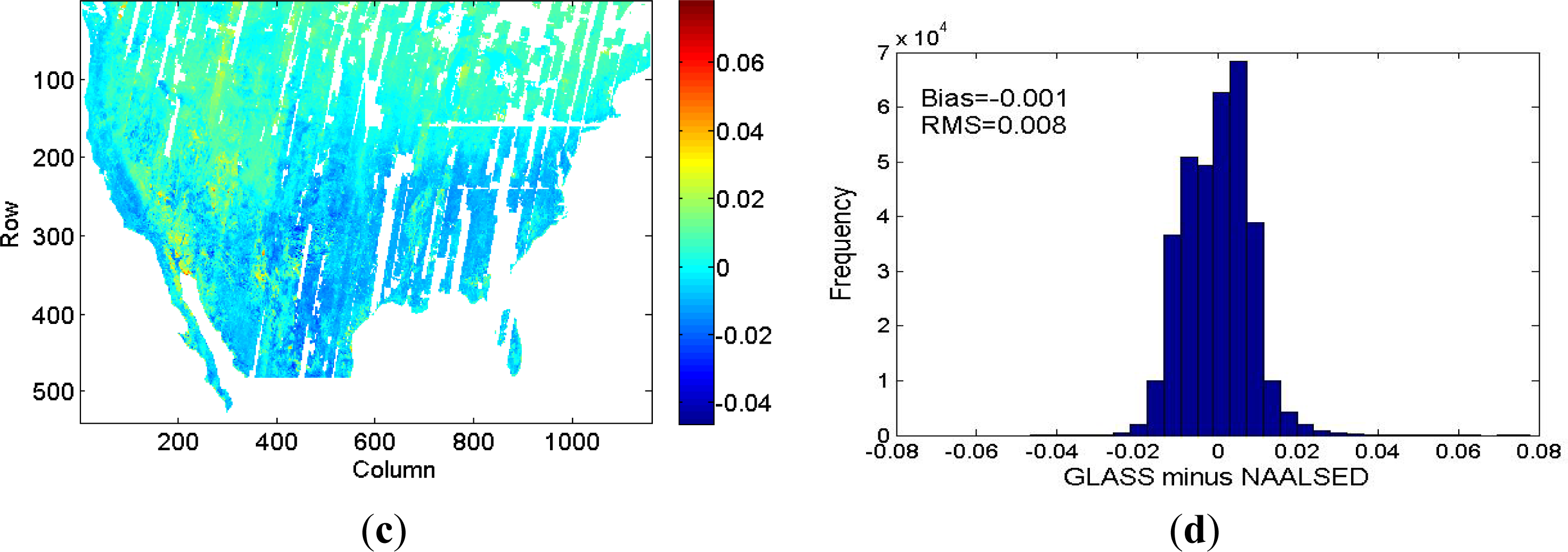
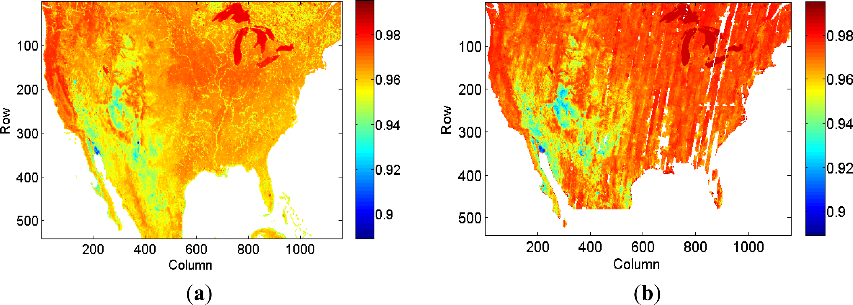
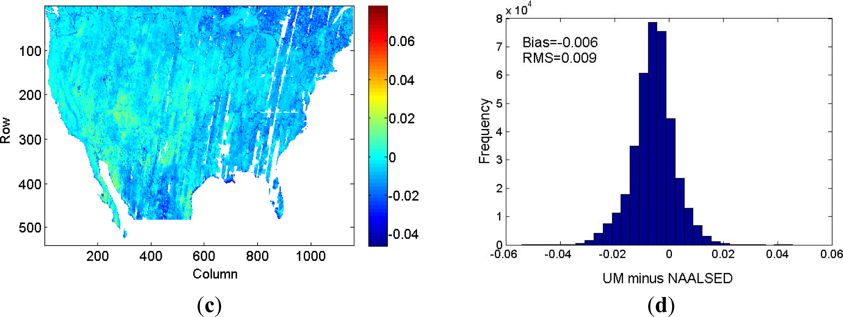
4.1. Compare to NAALSED BBE

Figures 1 and 2 show the comparison results between NAALSED BBE and GLASS BBE for the summer season and winter season, respectively. Note that the display difference in the Great Lakes was attributed to the use of different water/land masks. The BBE difference was calculated only at the pixel with both NAALSED BBE and GLASS BBE. Visually, GLASS BBE was more complete than NAALSED BBE, especially for the winter season. There was almost no missing data in the GLASS BBE while there were many gaps in the NAALSED BBE. The spatial pattern of NAALSED BBE and GLASS BBE were very similar. The BBE was relatively low in western semi-arid areas of the US, for example over the quartz-rich deserts of southeastern California, the Colorado Plateau, and the Grand Desierto in Mexico. The BBE was relatively high in the eastern agriculture areas of the US. In the western US, the GLASS BBE was larger than NAALSED BBE in summer season. In the northern US, the GLASS BBE was larger than NAALSED BBE in winter season. In general, GLASS BBE and NAALSED BBE were in good agreement. The bias and RMSE were −0.001 and 0.007 for the summer season, −0.001 and 0.008 for the winter season, respectively.

The comparison results between NAALSED BBE and UWIREMIS BBE are presented in Figures 3 and 4. Visually, UWIREMIS BBE was more complete than NAALSED BBE, especially for the winter season. The spatial pattern of UWIREMIS BBE and NAALSED BBE were very similar in the western US. The BBE was relatively low in the western semi-arid area. The UWIREMIS BBE was larger than NAALSED BBE in the western US. The UWIREMIS BBE and NAALSED BBE were quite different in the northeastern US. The UWIREMIS BBE was much lower than NAALSED BBE. The difference between UWIREMIS BBE and NAALSED BBE was smaller than that between GLASS BBE and NAALSED BBE in the western US, where the difference between UWIREMIS BBE and NAALSED BBE was larger than that between GLASS BBE and NAALSED BBE in the northeastern US. The bias and RMSE were −0.006 and 0.009 for the summer season, −0.008 and 0.011 for the winter season, respectively. It is evident that the GLASS BBE was closer to NAALSED BBE than UWIREMIS BBE. As described in Section 3.2, the BBE derived by converting ASTER emissivity has the highest accuracy in theory. So, the composited NAALSED BBE has the highest accuracy accordingly. Thus, the GLASS BBE was accurate than UWIREMIS BBE. Moreover, the validation studies indicated that the accuracy of 1 km GLASS BBE is 0.02 [30] whereas the UWIREMIS emissivity and UWIREMIS BBE are not validated.

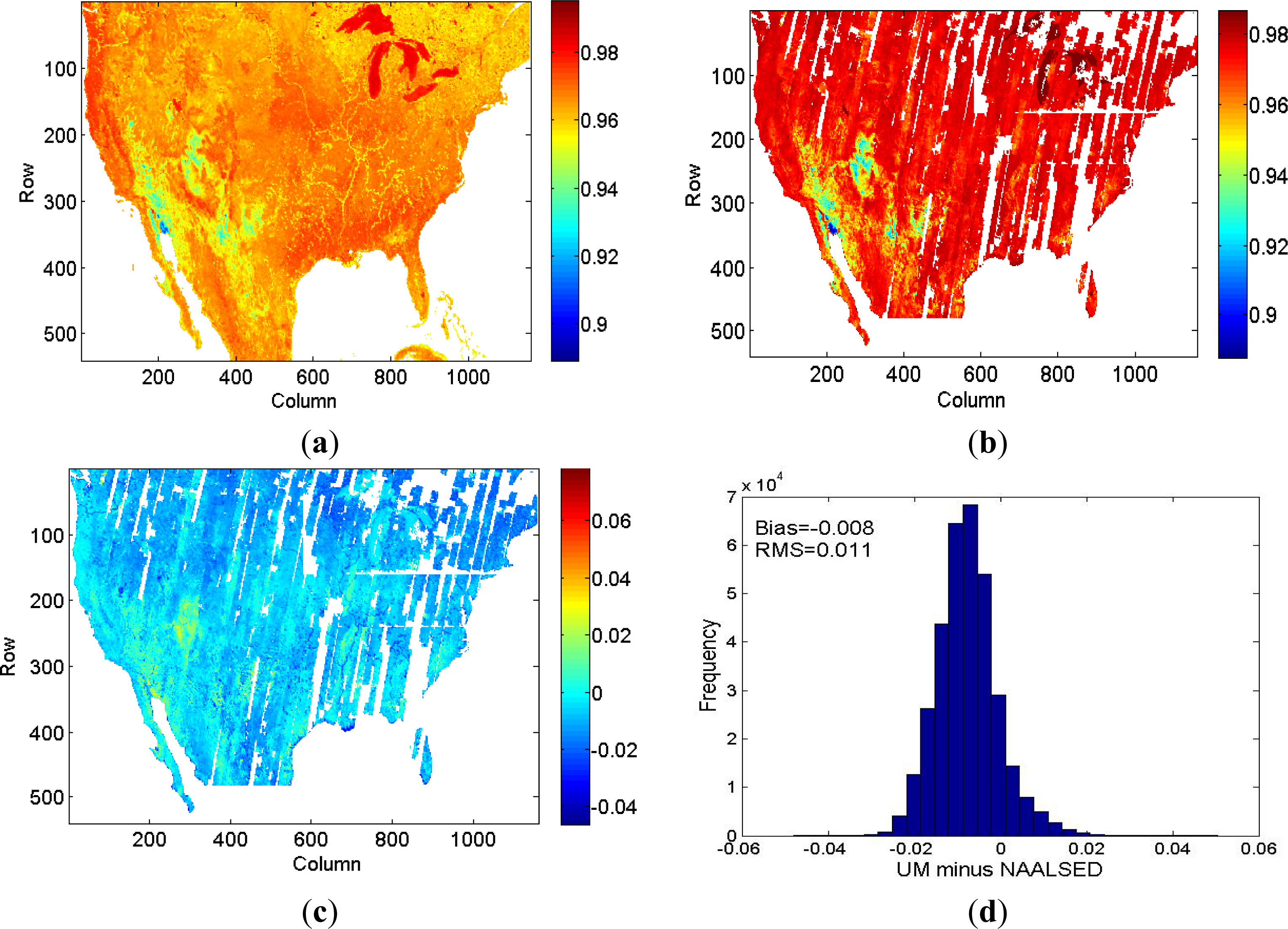
4.2. Comparison between UWIREMIS BBE and GLASS BBE

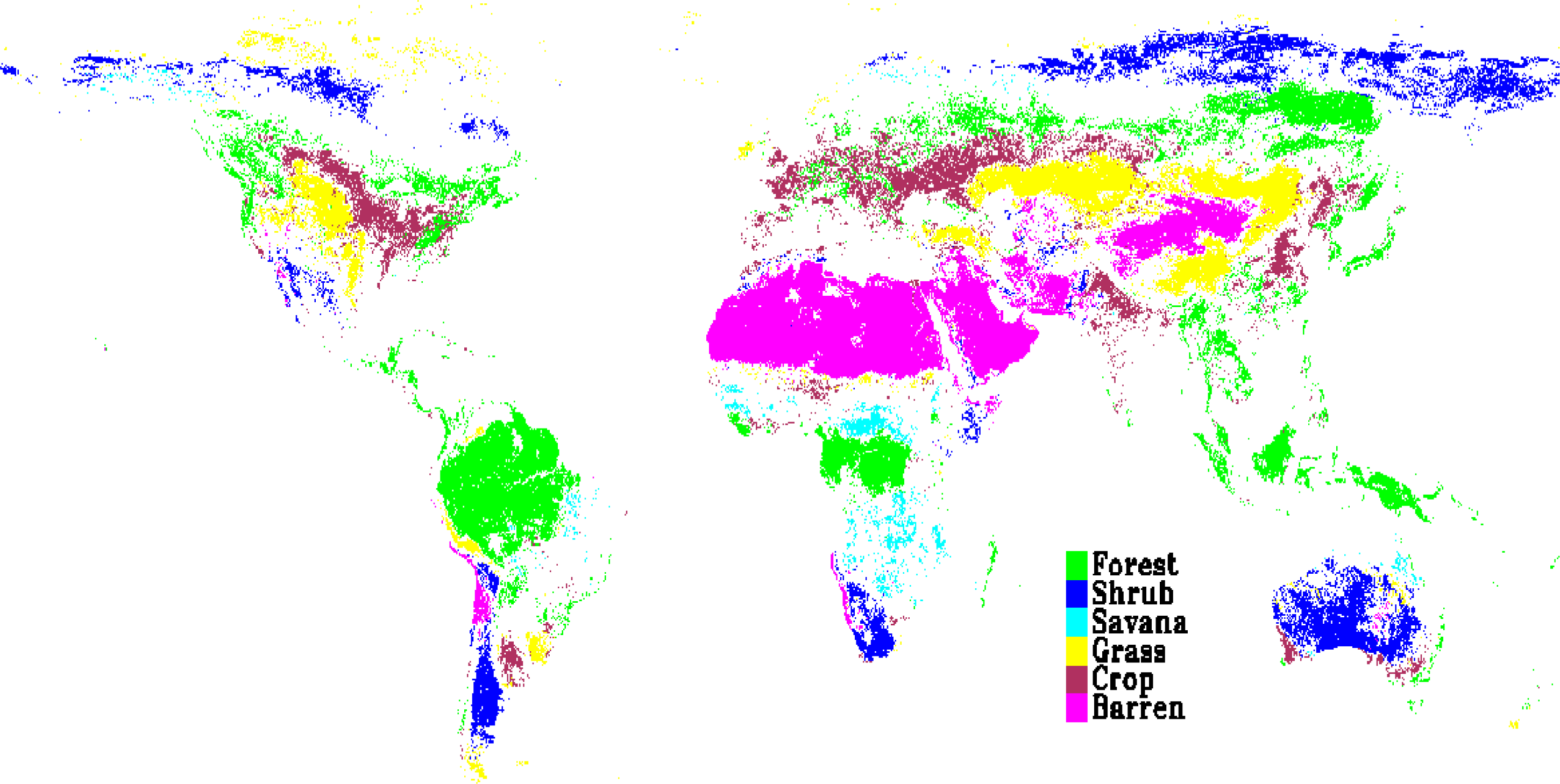
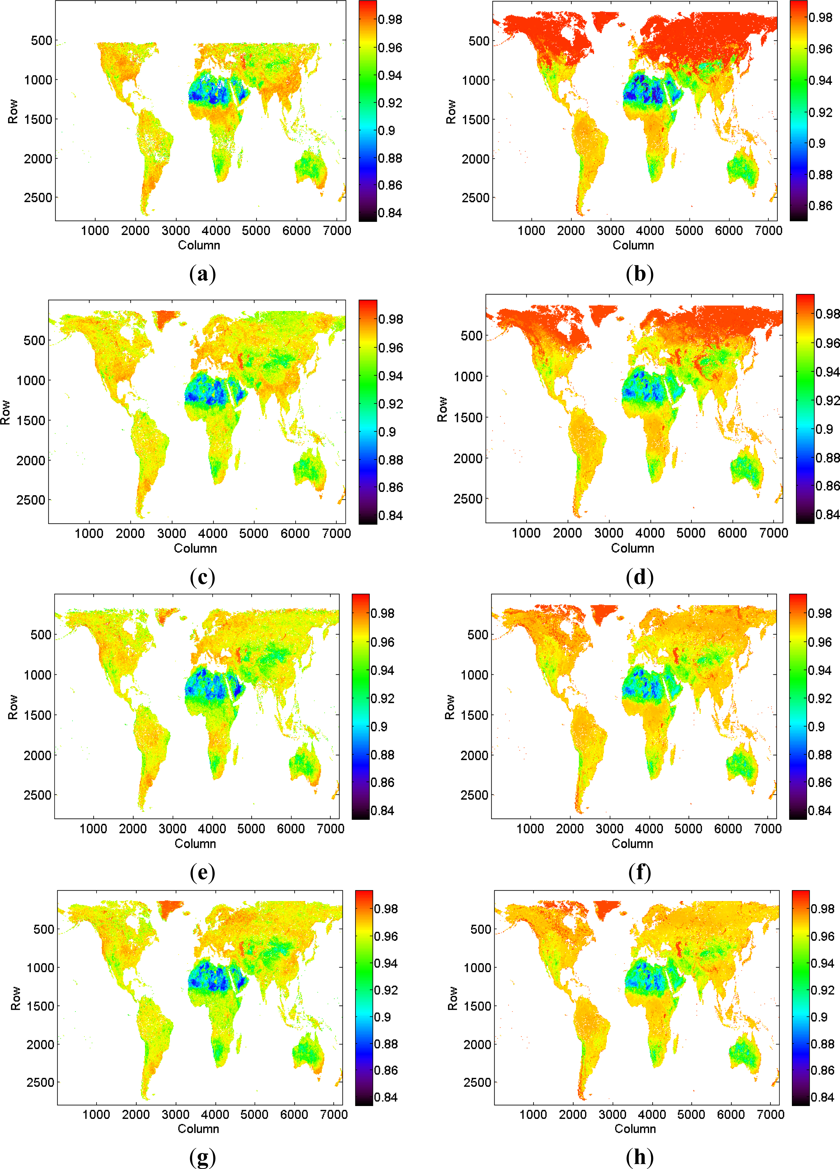
4.2.1. Spatial Distribution Pattern

Figure 5 presents the distribution of six dominant land cover types, combined from the 2003 MODIS Land cover product (MCD12C1). The global distribution of UWIREMIS BBE and GLASS BBE for four seasons (January, April, July and October) in 2003 is presented in Figure 6. In general, the BBE was very low over arid and semi-arid areas, for example, the Sahara Desert, northwest China, and the western United States. Shrub also had a lower BBE. The vegetated areas had relatively high BBE. The BBE for vegetated areas usually increases with the increasing of fractional vegetation cover, but the seasonal variation of BBE over vegetated areas cannot be seen from Figure 6 visually. In the algorithm for producing GLASS BBE, the BBE for snow/ice was assigned as 0.985. The UWIREMIS snow/ice BBE was calculated from emissivity at the four hinge points derived from the MODIS snow emissivity, which was retrieved by use of a physical-based day/night algorithm. The UWIREMIS snow/ice BBE was variable and does not exactly equal 0.985 at most conditions. The colors that represent snow/ice BBE were different in Figure 6. From the color of UWIREMIS BBE at Greenland, we can see the seasonal variation of snow cover. Most areas of Greenland were covered by snow in January and April, and most snow had melted in July. The UWIREMIS BBE was low in April and October in the northern part of Europe. This was unreasonable as both the snow and forest had relatively high BBE. The snow/ice flag was extracted from the MODIS reflectance product (MOD09A1) in the GLASS BBE algorithm. The snow cover variation for four seasons could be reflected from the GLASS BBE variations. The high latitude area was covered by snow in January, and the snow began to melt with the passage of time. There was almost no snow cover in July except in Greenland. By October, snow fall was present at high latitudes.

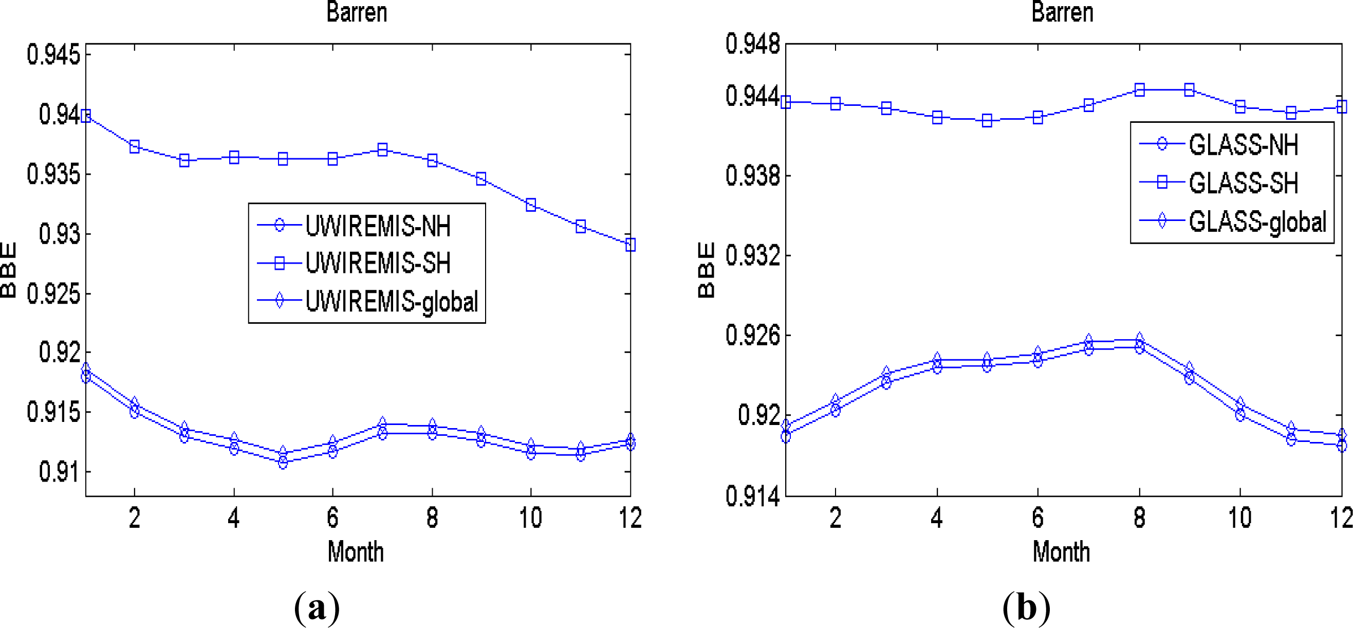
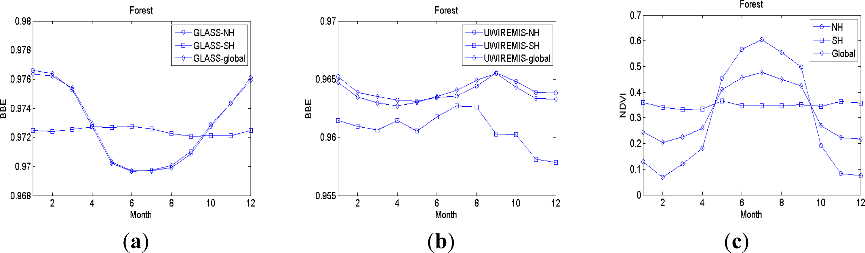
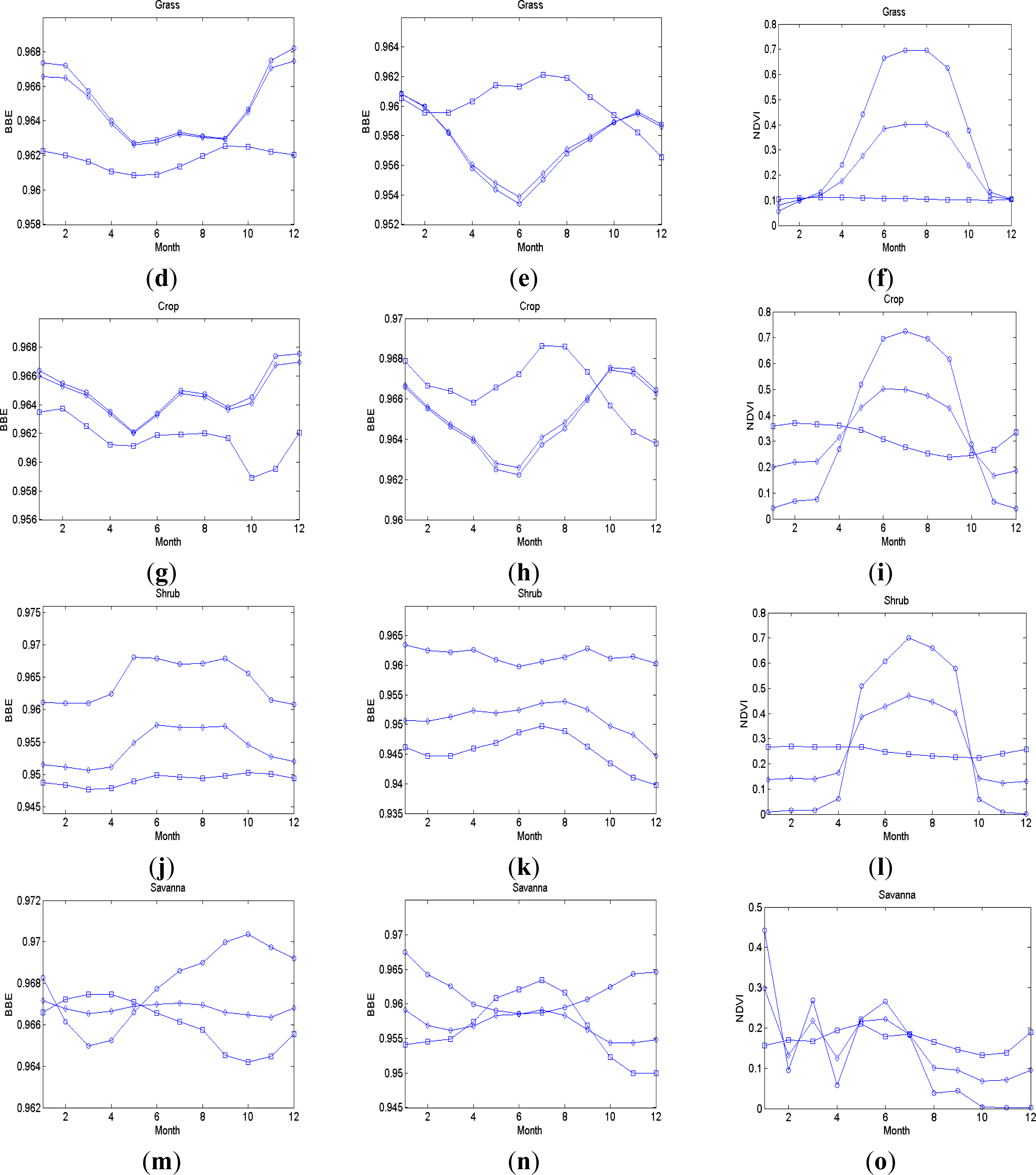
4.2.2. Seasonal Pattern

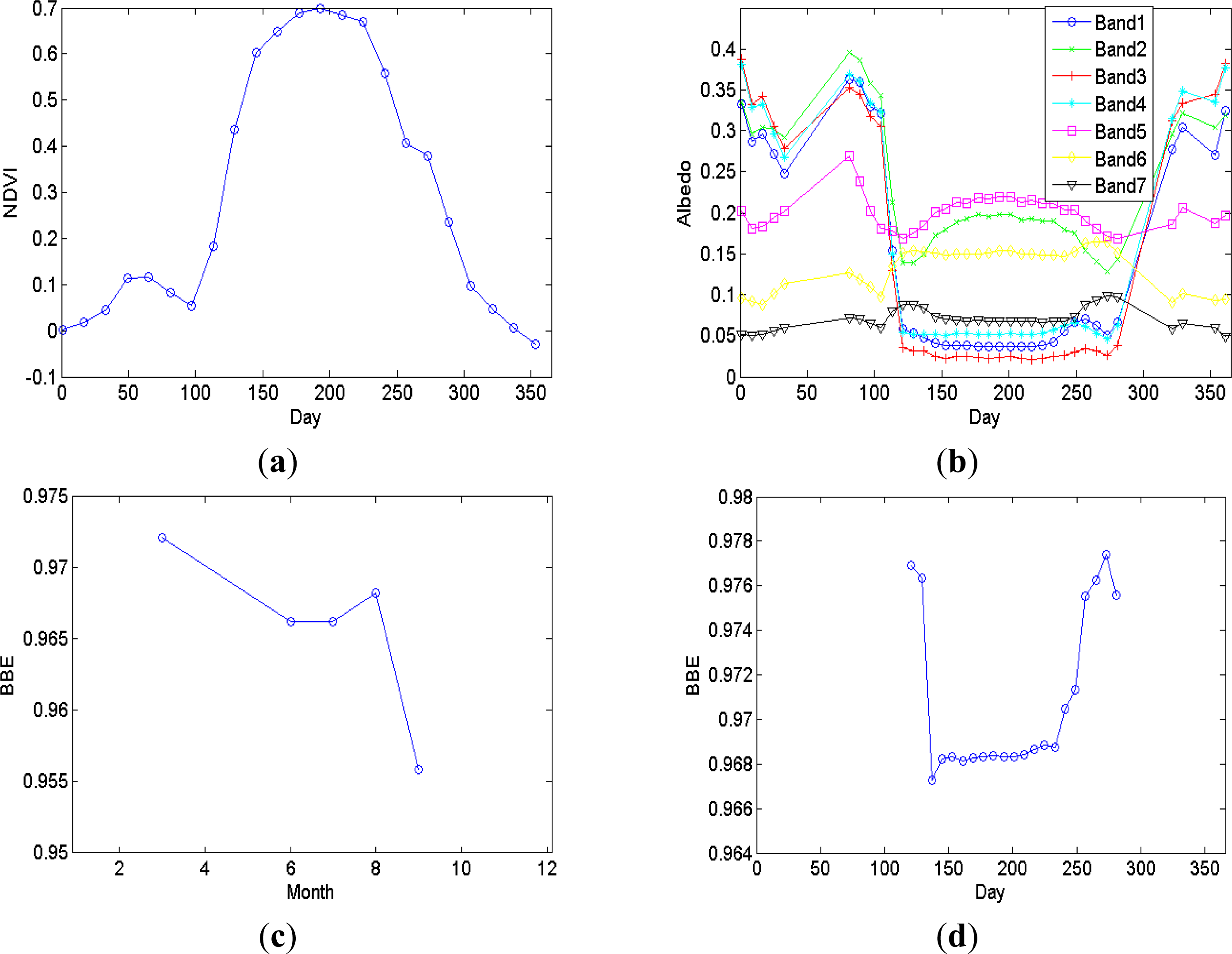
The monthly average BBE for barren is presented in Figure 7. The Northern Hemisphere (NH) GLASS BBE in summer was larger than that in winter and almost constant in the Southern Hemisphere (SH). The UWIREMIS BBE exhibited a decline trend from January to December in the NH and SH. The variation of both global GLASS BBE and UWIREMIS BBE were similar to variation in NH. The soil moisture is the main factor that influenced its emissivity. The soil emissivity increase with the increasing of water content before it is Saturation. The soil moisture in summer is higher than that in winter in the NH. The soil moisture is not a predictor in the GLASS BBE algorithm. The seasonal variation of GLASS BBE over barren is consistent with that of the soil moisture in the NH. Thus, the variation of GLASS BBE over barren in the NH seems more reasonable than that of UWIREMIS BBE.

The monthly average BBE for five vegetated land cover types calculated from UWIREMIS BBE and GLASS BBE respectively is presented in Figure 8. In order to better analyze the seasonal variation of vegetated land cover types, we also calculated the monthly average NDVI using the MODIS vegetation index product (MOD13C2) from 2003 through 2006. As shown in Figure 8, the variation of NDVI was coincided with the growth season of vegetation in NH (from May to September). The NDVI started from a lower value in winter, increased gradually from spring season until July when the NDVI achieved the maximum. Then, NDVI decreased gradually and reached a lower value again in winter season. In SH, the variation of NDVI is quite small. Generally, the emissivity of vegetation canopy is higher than that of bare soil. The emissivity of mixed pixel composed of vegetation canopy and bare soil increases with an increase of fractional vegetation cover [47–49]. The fractional vegetation cover can be represented by the NDVI. Thus, the seasonal variation of BBE should coincide with the seasonal variation of NDVI. However, this is not the case for both GLASS BBE and UWIREMIS BBE.

The seasonal variation of SH GLASS BBE was very small, while the seasonal variation of NH GLASS BBE was opposite to that of NDVI, except for savanna. According to the NDVI of savanna, we can judge that savanna belongs to a sparsely vegetated pixel whose emissivity was controlled mainly by the emissivity of bare soil. The seasonal variation of NH GLASS BBE resembled a cosine curve and the BBE of the growth season is lower than that of the non-growth season in NH for forest, grass, and crop. The seasonal variation of GLASS BBE for shrub agreed well with the variation of NDVI. The seasonal variation of global GLASS BBE was similar to that of NH GLASS BBE except for that for savanna. By contrast, the seasonal variation of UWIREMIS BBE in global and NH was similar to that of GLASS BBE for grass and crop. The seasonal variation of global and NH UWIREMIS BBE was very small for forest. The seasonal variation of UWIREMIS BBE in SH is larger than that of GLASS BBE in SH, and exhibits a peak value in summer for forest, grass, crop and savanna. The seasonal variation of UWIREMIS BBE was very small for shrub. In conclusion, the seasonal variation of GLASS BBE is more reasonable that that of UWIREMIS BBE and even GLASS BBE cannot reflect the seasonal variation of fractional vegetation cover for most vegetated land cover types.

According to the studies of Wang and Liang [50], the seasonal variation of monthly BBE derived by converting MODIS narrowband emissivity product during 2002 and 2006 was very small, and the monthly BBE derived by converting ASTER narrowband emissivity during 2000 and 2007 in summer was lower than that in winter over six surface radiation budget observing network (SURFRAD) sites (Bondville, Boulder, Fort Peck, Goodwin Creek, Penn State and Sioux Falls). We can deduce that MODIS narrowband emissivity lack seasonal variation because the used coefficients for converting narrowband emissivity to broadband are all positive. Furthermore, the temporal information was not considered in the baseline fit method [20]. So, it is not difficult to understand why UWIREMIS BBE lacks seasonal variation. As the ASTER BBE in summer is lower than that in winter, GLASS BBE in summer is likely to be lower than that in winter for the reason that the algorithm for retrieving GLASS BBE established the linear relationship between ASTER BBE and MODIS black-sky albedos.

We first calculated the average NAALSED BBE, GLASS BBE and UWIREMIS BBE for summer and winter seasons with data used in Section 3.2. The results are presented in

Table 1. Seasonal average BBE for six land cover types calculated from the data used in Section 3.2.

Data Set	Forest	Grass	Crop	Shrub	Savanna	Barren
Summer Season
NAALSED	0.975±0.003	0.966±0.007	0.972±0.005	0.952±0.010	0.972±0.005	0.938±0.017
GLASS	0. 971±0.003	0. 965±0.005	0. 967±0.004	0. 959±0.007	0. 968±0.002	0. 951±0.017
UWIREMIS	0.965±0.008	0.962±0.007	0.967±0.006	0.951±0.010	0.959±0.006	0.940±0.015
Winter Season
NAALSED	0.977±0.003	0.974±0.005	0.974±0.005	0.960±0.010	0.974±0.002	0.939±0.021
GLASS	0.977±0.006	0.969±0.009	0.969±0.005	0.957±0.003	0.966±0.002	0.946±0.018
UWIREMIS	0.963±0.007	0.964±0.006	0.966±0.006	0.956±0.008	0.968±0.005	0.941±0.015

. NAALSED BBE in summer was lower than that in winter for all the six land cover types. GLASS BBE in summer was lower than that in winter for forest, grass and crop, and GLASS BBE in summer was higher than that in winter for shrub, savanna and barren. UWIREMIS BBE in summer was lower than that in winter for grass, shrub, savanna and barren, and UMIREMIS BBE in summer was higher than that in winter for forest and crop. These results indicated that seasonal variation is incorrectly characterized in North America by all three BBE datasets. For NAALSED BBE and UWIREMIS BBE, this poor seasonal characterization can be ascribed to poor seasonal variation of the ASTER and MODIS narrowband emissivity. Regarding the GLASS BBE, its seasonal variation was influenced by both ASTER narrowband emissivity and MODIS spectral albedos. Taking deciduous needle leaf forest land cover as an example, we selected a homogeneous site (the land cover remained unchanged from 2001 through 2010; the central location: 59.8°N, 128.7°E) from MODIS land cover product, and downloaded the ASTER narrowband emissivity product, MODIS vegetation index product and MODIS albedo product. The MODIS and ASTER data were spatial matched. We averaged the NDVI and spectral albedos for 3 × 3 MODIS pixels, and averaged ASTER narrowband emissivity from 33 × 33 ASTER pixels. The ASTER BBE was calculated from averaged ASTER narrowband emissivities. We also calculated the corresponding BBE using GLASS BBE algorithm for vegetation with MODIS spectral albedos. The result is shown in Figure 9. As seen from Figure 9a, the NDVI increased gradually from spring and achieved the maximum in summer, then begun to decrease and achieved the minimum in winter; Figure 9b shows the corresponding MODIS spectral albedos. In growth season, the variation of first four albedos was contrary to the variation of NDVI, as the albedos tend to decrease with the increasing amount of vegetation. The seasonal variation of last three albedos was very small, as they did not reflect the growth of vegetation. Figure 9c presents the calculated ASTER BBE. The maximum occurred in March and the minimum appeared in September. Overall, the ASTER BBE did not exhibit seasonal variation. The derived GLASS BBE is provided in Figure 9d. Its seasonal variation resembled that of MODIS first four albedos. By comparing Figures 9b and 9d, we can see clearly that the variation of GLASS BBE is mainly determined by the seasonal variation of MODIS spectral albedos. In order to better characterize land surface [51,52], both the ASTER narrowband emissivity and MODIS narrowband emissivity products should be improved to consider the seasonal variation for vegetated areas. We are improving the GLASS BBE algorithm for vegetation to incorporate the seasonal variation of vegetation.

4.2.3. Time Series

The spatial-temporal matched GLASS BBE and UWIREMIS BBE were used to calculate the time series from 2003 through 2010. For GLASS BBE, there were regular periodic variations globally for crop, forest, grass, shrub and barren. The change trend for savanna was not significant. Regarding UWIREMIS BBE, there were regular periodic variations globally for crop. For forest, grass and shrub, the times series did not show periodic variations. The change trend of time series for savanna was similar to that derived from the GLASS BBE. The regular periodic variations for barren were quite weak. The periodic variations of GLASS BBE were stronger than that of UWIREMIS BBE, as we can clearly see from Figure 9. Figure 10 displays the temporal variations of GLASS BBE globally for a few major land cover types randomly selected from areas with relatively homogeneous land cover. There were some minor disagreements of BBE from AVHRR and MODIS data, but overall the long-term values were stable and consistent. In comparison, the UWIREMIS BBE values had much larger variations for most land cover types.

5. Conclusions

In this study, we compared three land surface BBE datasets. The first is a new global land surface BBE dataset known as GLASS BBE. The left two are NAALSED BBE and UWIREMIS BBE, which were calculated from two independent narrowband emissivity products, respectively. NAALSED BBE was taken as the reference for the good validation performance of ASTER narrowband emissivity product to evaluate the GLASS BBE and UWIREMIS BBE. These two BBE were more complete than NAALSED BBE, especially during the winter season. There were almost no gaps in these two BBE whereas the gaps in the NAALSED BBE can be easily seen elsewhere. The GLASS BBE was in good agreement with the NAALSED BBE for both the summer season and winter season. The bias and RMSE were −0.001 and 0.007 for the summer season, −0.001 and 0.008 for the winter season, respectively. The difference between UWIREMIS BBE and NAALSED BBE was larger than that between GLASS BBE and NAALSED BBE. The bias and RMSE were −0.006 and 0.009 for summer season, −0.008 and 0.011 for winter season, respectively. GLASS BBE was more accurate than UWIREMIS BBE.

The spatial distributions of GLASS BBE and UWIREMIS BBE in 2003 for six land cover types were compared. The BBE difference between vegetated areas (e.g., crop, forest, savanna, grass and shrub) and non-vegetated (barren) can be easily seen. However, the seasonal variation of BBE for vegetated areas was hard to find. The snow cover variation for four seasons could be reflected from the BBE variations. The monthly average BBE for six land cover types were calculated from UWIREMIS BBE and GLASS BBE ranging from 2003 through 2006, based on which we analyzed the seasonal pattern of two BBE datasets. For barren, GLASS BBE can reflect its seasonal variation while UWIREMIS BBE failed. Regarding vegetated areas, the seasonal variation of GLASS BBE was more reasonable that that of UWIREMIS BBE even GLASS BBE cannot reflect the seasonal variation of fractional vegetation cover for most vegetated land cover types. The time series were calculated from GLASS BBE and UWIREMIS BBE using the data from 2003 through 2010. The periodic variations of GLASS BBE were stronger than those of UWIREMIS BBE. The temporal variations of GLASS BBE globally for a few major land cover types randomly selected from areas with relatively homogeneous land cover. There were some minor disagreements of BBE from AVHRR and MODIS data, but overall the long-term values were stable and consistent. In comparison, the UWIREMIS BBE values had much larger variations for most land cover types.

In conclusion, GLASS BBE is the first global long time series land surface BBE dataset of high quality, and can be used in calculating surface longwave net radiation and incorporated in land surface models for improving model simulation results. We are improving the algorithm to better characterize the seasonal variation of vegetated land cover types.

References

1. Liang, S.; Wang, K.; Zhang, X.; Wild, M. Review of estimation of land surface radiation and energy budgets from ground measurements, remote sensing and model simulation. IEEE J. Sel. Top. Appl. Earth Obs. Remote Sens 2010, 3, 225–240. [Google Scholar]
2. Zhou, L.; Goldberg, M.; Barnet, C.; Cheng, Z.; Sun, F.; Wolf, W.; King, T.; Liu, X.; Sun, H.; Divakarla, M. Regression of surface spectral emissivity from hyperspectral instruments. IEEE Trans. Geosci. Remote Sens 2008, 46, 328–333. [Google Scholar]
3. Vogel, R.L.; Liu, Q.-H.; Han, Y.; Wend, F.-Z. Evaluating a satellite-derived global infrared land surface emissivity data set for use in radiative transfer modeling. J. Geophys. Res 2011, 116. [Google Scholar] [CrossRef]
4. Dickinson, R.E. Land Processes in climate models. Remote Sens. Environ 1995, 51, 27–38. [Google Scholar]
5. Yu, Y.; Tarpley, D.; Privette, J.L.; Flynn, L.E.; Xu, H.; Chen, M.; Vinnikov, K.Y.; Sun, D.; Tian, Y. Validation of GOES-R satellite land surface temperature algorithm using SURFRAD ground measurements and statistical estimates of error properties. IEEE Trans. Geosci. Remote Sens 2012, 50, 704–713. [Google Scholar]
6. Cheng, J.; Liang, S.; Liu, Q.; Li, X. Temperature and emissivity separation from ground-based MIR hyperspectral data. IEEE Trans. Geosci. Remote Sens 2011, 49, 1473–1484. [Google Scholar]
7. Xue, Y.; Lawrence, S.P.; Llewellyn-Jones, D.T.; Mutlow, C.T. On the Earth’s surface energy exchange determination from ERS satellite ATSR data. Part I: Long-wave radiation. Int. J. Remote Sens 1998, 19, 2561–2583. [Google Scholar]
8. Zhou, J.; Chen, Y.; Zhang, X.; Zhan, W. Modelling the diurnal variations of urban heat islands with multi-source satellite data. Int. J. Remote Sens 2013, 34, 7568–7588. [Google Scholar]
9. Bonan, G.B.; Oleson, K.W.; Vertenstein, M.; Levis, S.; Zeng, X.; Dai, Y.; Dickinson, R.E.; Yang, Z. The land surface climatology of the community land model coupled to the NCAR community climate model. J. Clim 2002, 15, 3123–3149. [Google Scholar]
10. Jin, M.; Liang, S. An improved land surface emissivity parameter for land surface models using global remote sensing observations. J. Clim 2006, 19, 2867–2881. [Google Scholar]
11. Sellers, P.J.; Mintz, Y.; Sud, Y.C.; Dalcher, A. A simple biosphere model (SiB) for use within general circulation models. J. Atmos. Sci 1986, 43, 505–531. [Google Scholar]
12. Zhou, L.; Dickinson, R.E.; Tian, Y.; Jin, M.; Ogawa, K.; Yu, H.; Schmugge, T. A sensitivity study of climate and energy blance simulations with use of satellite-based emissivity data over northern africa and the arabian peninsula. J. Geophys. Res 2003, 108. [Google Scholar] [CrossRef]
13. Wilber, A.C.; Kratz, D.P.; Gupta, S.K. Surface Emissivity Maps for Use in Satellite Retrievals of Longwave Radiation; NASA/TP-1999-209362; NASA Langley Research Center: Hampton, VA, USA, 1999; Available online: http://techreports.larc.nasa.gov/1trs (accessed on 13 December 2013).
14. Ogawa, K.; Schmugge, T. Mapping surface broadband emissivity of the sahara desert using ASTER and MODIS data. Earth Interact 2004, 8, 1–14. [Google Scholar]
15. Ogawa, K.; Schmugge, T.; Rokugawa, S. Estimating broadband emissivity of arid regions and its seasonal variations using thermal infrared remote sensing. IEEE Trans. Geosci. Remote Sens 2008, 46, 334–343. [Google Scholar]
16. Peres, L.F.; DaCamara, C.C. Emissivity maps to retrieve land-surface temperature from MSG/SEVIRI. IEEE Trans. Geosci. Remote Sens 2005, 43, 1834–1844. [Google Scholar]
17. Cheng, J.; Liang, S.; Yao, Y.; Zhang, X. Estimating the optimal broadband emissivity spectral range for calculating surface longwave net radiation. IEEE Geosci. Remote Sens. Lett 2013, 10, 401–405. [Google Scholar]
18. Liang, S. Quantitative Remote Sensing of Land Surface; John Wiley and Sons, Inc: Hoboken, NJ, USA, 2004. [Google Scholar]
19. Hulley, G.C.; Hook, S.J. The North American ASTER Land Surface Emissivity Database (NAALSED) Version 2.0. Remote Sens. Environ 2009, 113, 1967–1975. [Google Scholar]
20. Seemann, S.W.; Borbas, E.E.; knuteson, R.O.; Stephenson, G.R.; Huang, H.-L. Development of a global infrared land surface emissivity database for application to clear sky sounding retrieval from multispectral satellite radiance measurements. J. Appl. Meteorol. Climatol 2008, 47, 108–123. [Google Scholar]
21. Capelle, V.; Chedin, A.; Pequignot, E.; Schlussel, P.; Newman, S.M.; Scott, S.A. Infrared continental surface emissivity spectra and skin temperature retrieved from IASI observations over the tropics. J. Appl. Meteorol. Climatol 2012, 51, 1164–1179. [Google Scholar]
22. Zhou, D.K.; Larar, A.M.; Liu, X.; Smith, W.L.; Strow, L.L.; Yang, P.; Schlussel, P.; Calbet, X. Global land surface emissivity retrieved from satellite ultraspectral IR measurements. IEEE Trans. Geosci. Remote Sens 2011, 49, 1227–1290. [Google Scholar]
23. Li, J.; Li, J.-L. Derivation of a global hyperspectral resolution surface emissivity spectra from advanced infrared sounder radiance measurements. Geophys. Res. Lett 2008, 35, L15807. [Google Scholar] [CrossRef]
24. susskind, J.; Blaisdell, J. Improved surface parameter retrievals using AIRS/AMSU data. Proc. SPIE 2008, 6966. [Google Scholar] [CrossRef]
25. Aumann, H.; Chanhine, M.T.; Gautier, C. AIRS/AMSU/HSB on the AQUA mission: Design, science objectives, data products, and processing systems. IEEE Trans. Geosci. Remote Sens 2003, 41, 253–264. [Google Scholar]
26. Trigo, I.F.; Peres, L.F.; DaCamara, C.C.; Freitas, S.C. Thermal land surface emissivity retrieved from SEVIRI/Meteosat. IEEE Trans. Geosci. Remote Sens 2008, 46, 307–315. [Google Scholar]
27. Cheng, J.; Liang, S. Estimating the broadband longwave emissivity of global bare soil from the MODIS shortwave albedo product. J. Geophys. Res.: Atmos 2013. [Google Scholar] [CrossRef]
28. Cheng, J.; Liang, S. Estimating global land surface broadband thermal-infrared emissivity from the advanced very high resolution radiometer optical data. Int. J. Digit. Earth 2013. [Google Scholar] [CrossRef]
29. Liang, S.; Zhao, X.; Liu, S.; Yuan, W.; Cheng, X.; Xiao, Z.; Zhang, X.; Liu, Q.; Cheng, J.; Tang, H.; et al. A long-term Global LAnd Surface Satellite (GLASS) data-set for environmental studies. Int. J. Digit. Earth 2013. [Google Scholar] [CrossRef]
30. Dong, L.X.; Hu, J.Y.; Tang, S.H.; Min, M. Field validation of GLASS land surface broadband emissivity database using pseudo-invariant sand dunes sites in northern China. Int. J. Digit. Earth 2013. [Google Scholar] [CrossRef]
31. Liang, S.; Zhang, X.; Xiao, Z.; Cheng, J.; Liu, Q.; Zhao, X. Global LAnd Surface Satellite (GLASS) Products: Algorithm, Validation and Analysis; Springer: Berlin, Germany, 2013. [Google Scholar]
32. Ren, H.; Liang, S.; Yan, G.; Cheng, J. Empirical algorithms to map global broadband emissivities over vegetated surfaces. IEEE Trans. Geosci. Remote Sens 2013, 51, 2619–2631. [Google Scholar]
33. Baldridge, A.M.; Hook, S.J.; Grove, C.I.; Rivera, G. The ASTER spectral library version 2.0. Remote Sens. Environ 2009, 113, 711–715. [Google Scholar]
34. Cheng, J.; Liang, S.; Weng, F.; Wang, J.; Li, X. Comparison of radiative transfer models for simulating snow surface thermal infrared emissivity. IEEE J. Sel. Top. Appl. Earth Obs. Remote Sens 2010, 3, 323–336. [Google Scholar]
35. Hulley, G.C.; Hook, S.J. A new methodology for cloud detection and calssification with ASTER data. Geophys. Res. Lett 2008, 35. [Google Scholar] [CrossRef]
36. Hulley, G.C.; Hook, S.J.; Baldridge, A.M. Validation of the North American ASTER Land Surface Emissivity Database (NAALSED) version 2.0 using pseudo-invariant sand dune sites. Remote Sens. Environ 2009, 113, 2224–2233. [Google Scholar]
37. Hapke, B. Theory of Reflectance and Emittance Spectroscopy; Cambridge Unviersity Press: New York, NY, USA, 1993. [Google Scholar]
38. Cheng, J.; Liang, S. Effects of thermal-infrared emissivity directionality on surface broadband emissivity and longwave net radiation estimation. IEEE Geosci. Remote Sens. Lett 2014, 11, 499–503. [Google Scholar]
39. Du, Y.; Liu, Q.-H.; Chen, L.-F.; Liu, Q.; Yu, T. Modeling directional brightness temperature of the winter wheat canopy at the ear stage. IEEE Trans. Geosci. Remote Sens 2007, 45, 3721–3739. [Google Scholar]
40. Gillespie, A.R.; Rokugawa, S.; Matsunaga, T.; Cothern, J.S.; Hook, S.J.; Kahle, A.B. A temperature and emissivity separation algorithm for Advanced Spaceborne Thermal Emission and Reflection Radiometer (ASTER) images. IEEE Trans. Geosci. Remote Sens 1998, 36, 1113–1126. [Google Scholar]
41. Gillespie, A.R.; Abbott, E.A.; Gilson, L.; Hulley, G.; Jimenez-Munoz, J.-C.; Sobrino, J.A. Residual errors in ASTER temperature and emissivity products AST08 and AST05. Remote Sens. Environ 2011, 115, 3681–3694. [Google Scholar]
42. Sabol, D.E., Jr.; Gillespie, A.R.; Abbott, E.; Yamada, G. Field validation of the ASTER Temperature-Emissivity Separation Algorithm. Remote Sens. Environ 2009, 113, 2328–2344. [Google Scholar]
43. Mira, M.; Schmugge, T.J.; Valor, E.; Caselles, V.; Coll, C. Analysis of ASTER emissivity product over an arid area in southern New Mexico, USA. IEEE Trans. Geosci. Remote Sens 2011, 49, 1316–1324. [Google Scholar]
44. Matsunaga, T.; Sawabe, Y.; Rokugawa, S.; Tonooka, H.; Moriyama, M. Early evaluation of ASTER emissivity products and its application to environmental and geologic studies. Proc. SPIE 2001, 4486. [Google Scholar] [CrossRef]
45. Jimenez-Munoz, J.C.; Sobrino, J.A.; Gillespie, A.; Sabol, D.; Gustafson, W.T. Improved land surface emissivities over agricultural areas using ASTER NDVI. Remote Sens. Environ 2006, 103, 474–487. [Google Scholar]
46. Gustafson, W.T.; Gillespie, A.R.; Yamada, G.J. Revisions to the ASTER Temperature/Emissivity Separation Algorithm. In Second Recent Advances in Quantitative Remote Sensing; Sobrino, J.A., Ed.; Universitat de Valencia: Valencia, Spain, 2006; pp. 770–775. [Google Scholar]
47. Griend, A.A.V.D.; Owe, M. On the relationship between thermal emissivity and the normalized difference vegetation index for natural surfaces. Int. J. Remote Sens 1993, 14, 1119–1131. [Google Scholar]
48. Valor, E.; Caselles, V. Mapping land surface emissivity from NDVI: Application to European, African, and South American areas. Remote Sens. Environ 1996, 57, 167–184. [Google Scholar]
49. Snyder, W.C.; Wan, Z. BRDF modles to predict spectral reflectance and emissivity in the thermal infrared. IEEE Trans. Geosci. Remote Sens 1998, 36, 214–225. [Google Scholar]
50. Wang, K.; Liang, S. Evaluation of ASTER and MODIS land surface temperature and emissivity products usning long-term surface longwave radiation observations at SURFRAD sites. Remote Sens. Environ 2009, 113, 1556–1565. [Google Scholar]
51. French, A.N.; Schmugge, T.J.; Ritchie, J.C.; Hsu, A.; Jacob, F.; Ogawa, K. Detecting land cover change at the Jornada Experimental Rang, New Mexico with ASTER emissivities. Remote Sens. Environ 2008, 112, 1730–1748. [Google Scholar]
52. French, A.N.; Inamdar, A. Land cover characterization for hydrological modelling using thermal infrared emissivities. Int. J. Remote Sens 2010, 31, 3867–3883. [Google Scholar]
Figure 1. Comparison between NAALSED BBE and GLASS BBE for summer season. (a) GLASS BBE; (b) NAALSED BBE; (c) the difference between GLASS BBE and NAALSED BBE; (d) the histogram of the difference.
Remotesensing 06 00111f1
Figure 2. Comparison between NAALSED BBE and GLASS BBE for winter season. (a) GLASS BBE; (b) NAALSED BBE; (c) the difference between GLASS BBE and NAALSED BBE; (d) the histogram of the difference.
Remotesensing 06 00111f2aRemotesensing 06 00111f2b
Figure 3. Comparison between NAALSED BBE and UWIREMIS BBE for the summer season. (a) UWIREMIS BBE; (b) NAALSED BBE; (c) the difference between UWIREMIS BBE and NAALSED BBE; (d) the histogram of the difference.
Remotesensing 06 00111f3aRemotesensing 06 00111f3b
Figure 4. Comparison between NAALSED BBE and UWIREMIS BBE for the winter season. (a) UWIREMIS BBE; (b) NAALSED BBE; (c) the difference between UWIREMIS BBE and NAALSED BBE; (d) the histogram of the difference.
Remotesensing 06 00111f4
Figure 5. Global distribution of six land cover types composited from 2003 MODIS land cover product.
Remotesensing 06 00111f5
Figure 6. Geographical distribution of global UWIREMIS BBE and GLASS BBE. (a) UWIREMIS January BBE; (b) GLASS January BBE; (c) UWIREMIS April BBE; (d) GLASS April BBE; (e) UWIREMIS July BBE; (f) GLASS July BBE; (g) UWIREMIS October BBE; (h) GLASS October BBE.
Remotesensing 06 00111f6
Figure 7. Monthly mean BBE of barren calculated from UWIREMIS BBE (a) and GLASS BBE (b) for global, North Hemisphere (NH) and South Hemisphere (SH), respectively.
Remotesensing 06 00111f7
Figure 8. Monthly mean BBE of five land cover types calculated from UWIREMIS BBE and GLASS BBE for global, North Hemisphere (NH) and South Hemisphere (SH), respectively. (a) GLASS Forest BBE; (b) UWIREMIS Forest BBE; (c) MODIS Forest NDVI; (d) GLASS Grass BBE; (e) UWIREMIS Grass BBE; (f) MODIS Grass NDVI; (g) GLASS Crop BBE; (h) UWIREMIS Crop BBE; (i) MODIS Crop NDVI; (j) GLASS Shrub BBE; (k) UWIREMIS Shrub BBE; (l) MODIS Shrub NDVI; (m) GLASS Savanna BBE; (n) UWIREMIS Savanna BBE; (o) MODIS Savanna NDVI.
Remotesensing 06 00111f8aRemotesensing 06 00111f8b
Figure 9. The calculated parameters for a homogeneous deciduous needle leaf forest site using coregistered MODIS and ASTER data from 2000 through 2010. (a) NDVI; (b) MODIS spectral albedo; (c) ASTER BBE; (d) GLASS BBE.
Remotesensing 06 00111f9
Figure 10. Time series of mean GLASS BBE and UWIREMIS BBE from years 2000–2010. (a) Forest; (b) Grass; (c) Crop; (d) Shrub; (e) Savanna; (f) Barren.
Remotesensing 06 00111f10aRemotesensing 06 00111f10b
Figure 11. Long-term global BBE of five land cover types from GLASS BBE and UWIREMIS BBE product. (a) Forest; (b) Grass; (c) Crop; (d) Savanna; (e) Barren.
Remotesensing 06 00111f11aRemotesensing 06 00111f11b