Now You See It… Now You Don’t: Understanding Airborne Mapping LiDAR Collection and Data Product Generation for Archaeological Research in Mesoamerica

 ,
, 
Abstract
: In this paper we provide a description of airborne mapping LiDAR, also known as airborne laser scanning (ALS), technology and its workflow from mission planning to final data product generation, with a specific emphasis on archaeological research. ALS observations are highly customizable, and can be tailored to meet specific research needs. Thus it is important for an archaeologist to fully understand the options available during planning, collection and data product generation before commissioning an ALS survey, to ensure the intended research questions can be answered with the resultant data products. Also this knowledge is of great use for the researcher trying to understand the quality and limitations of existing datasets collected for other purposes. Throughout the paper we use examples from archeological ALS projects to illustrate the key concepts of importance for the archaeology researcher.1. Introduction
During the past decade the laser pulse rates of commercially manufactured airborne mapping Light Detection and Ranging (LiDAR) systems, also known as Airborne Laser Scanning (ALS) systems have increased from several thousand pulses per second to hundreds of thousands of pulses per second—by about a factor of 50 to 100 [1]. Most units now record multiple stops (returns) per laser pulse, as well as the intensity (signal strength) of the reflected signal, and some digitize and record the full return signal or waveform. The immediate output from an ALS unit is a point cloud, consisting of the coordinates of unequally spaced points (returns) from which sufficient laser light has been reflected to be detected by the sensor. These “raw” point clouds are then processed using various algorithms [2] that may consider both the distribution and intensity of the returns, in order to classify the returns as most likely being from vegetation, human engineered structures, or the ‘bare earth.’ Or, when the ALS utilizes a laser with a wavelength that penetrates water, points may also be classified as most likely being from the surface, within, or the bottom of water bodies, including streams, lakes and near shore coastal waters [3].
Once all of the recorded returns have been classified, a variety of algorithms may be used to extract and display information sought for a particular application. Often the points identified as ground points are used to produce “bare earth” geodetic images (rasters that provide elevation information for an X, Y coordinate array), on which every element on the raster (image) is known in a well-defined geodetic and temporal reference frame. These rasters can also present other types of spectral and spatial information derived from the ALS observations such as return intensity or elevation variation (surface roughness) or return density.
The exponential development of ALS technology triggered an explosion in its use for archaeology with early applications in Europe [4–9] and one target of opportunity in Mesoamerica in 2001 [10]. However the application of the technique gained significant momentum for prospection in regions covered with dense vegetation, including the multi-layer tropical and sub-tropical rain forests of South and Central America [11,12], as well as South East Asia [13–15]. The ability to map landscapes hidden beneath dense vegetation is resulting in a revolution in archaeology arguably comparable to that caused by the introduction of radiocarbon dating some decades ago [13]. Also, as more and more work is being done, researchers have been invigorated with its potential and intrigued by its limitations. Questions include: How small an object can be detected [16,17]? How accurate are the data? Why are some features clearly visible in an area but not as clear in a different area, of the same project? Why do causeways, which are very difficult to see on the ground because of their small elevation relief, appear very clearly in the ALS observations, while other features with larger elevation relief are easy to spot on the ground, but are hard to spot with ALS data?
Often researchers compare ALS rasters with satellite or airborne imagery, and try to use analogies to compare and understand the information they contain. While there are some parallels, the datasets are more different than alike. Spaceborne or airborne imagery is generally highly standardized, and there is extensive documentation addressing all aspects of the collection and processing of the raw data into imagery products. On the other hand ALS data products and the procedures used to collect, reduce, and process the data into final deliverables are not standardized. Not all ALS products are created equal, nor should they be. The considerations and decisions made at each of the ALS data workflow steps affect the quality of the final products and hence their usefulness in answering specific research questions. It is important for the researcher to understand these decisions and options.
Archaeologists using data products derived from ALS observations need to understand the technology, be aware of its limitations, and be careful not to identify features that are not reliably captured by the ALS observations, or rule out the existence of features not detected by the observations. Our goal here is to use examples taken from archeological research projects to illustrate how ALS technology works, how data are collected, reduced and deliverables produced, and how decisions made at each of these steps impact the ability of the archeologist to answer the research questions.
The US National Science Foundation (NSF) National Center for Airborne Laser Mapping (NCALM) has over 15 years of experience of providing research quality LiDAR data for the scientific and engineering communities, and has been collecting ALS data for archaeological applications since 2008 in the US Southwest and Mesoamerica (Table 1. summarizes the project locations, surveyed areas, and nominal shot densities).
This paper is based on the analysis of data collected, results from sensor configuration experiments, and lessons learned from the execution of these projects; it is intended to complement and expand information presented in previous instructional works such as [18–20]. The present work complements the previously cited works in multiple ways with the two main ones being: (1) While the previous works provide brief high level overviews of ALS technology and LiDAR data acquisition their main focus is on how to process, analyze and visualize the data once it is delivered (post-production). In contrast the present work provides a deeper and more complete description of the technology with a focus on the collection and data product generation (pre-production and production) and how the decisions made by the ALS data provider at these stages can affect the ability of an investigator to answer research questions; (2) The cited works are based on the topographic, ecological and anthropological environments of Europe, while this work has been performed in the unique conditions of Mesoamerica. This work is intended to be as complete as a research paper allows, focusing on the archaeological application, however it is not an exhaustive coverage and therefore the reader is referred to the textbook and handbook style works [21–23] for additional general information on ALS systems and data products.
This paper is structured in the following way: In Section 2 we present an overview of ALS technology, data products and nomenclature, which will provide a base for the discussion on how different aspects of the technology affect the final results. Section 3 describes the ALS workflow and how the decisions and considerations made at each step may affect the final products and their usefulness in answering particular research questions. Finally in Section 4 we discuss LiDAR data visualization, analysis, quality assessment and how to evaluate the fidelity of structures evident on elevation rasters or other ALS datasets.
2. Understanding the Jargon: Equipment and Data Products
The acronym LiDAR stands for Light Detection and Ranging and for obvious reasons it is also called Optical Radar. The military community commonly uses the acronym LADAR, for Laser Detection and Ranging, to be specific about the type of light source used. Today the term LiDAR is used loosely and serves as an umbrella for different kinds of technologies and applications that range from using satellites to map atmospheric density, composition, and wind speed and direction; to close range 3D mapping of minute artifacts at micrometric resolution. For a historical description on the technology, nomenclature and diverse applications refer to [24].
In this paper our focus will be on the use of topographic mapping LiDAR from airborne platforms, commonly referred to as airborne laser scanning or ALS [1]. However, even within the smaller umbrella of ALS there are multiple types of LiDAR units that have or can be used for archeological applications, and each one has specific advantages or disadvantages with regard to providing information to answer a given research question for a given type of environment. For example a single stop LiDAR system might prove very efficient in mapping the thinly vegetated surface of a desert, but would be nearly useless in mapping the surface of the ground in an area covered by jungle canopy [25].
2.1. Understanding ALS Technology
To introduce and explain the taxonomy of ALS systems (Figure 1) we begin with the single function that all LiDAR units have in common: to measure the two-way travel time of light from the sensor to the target (Earth’s surface, vegetation, manmade structures, etc.). Today most, if not all, ALS systems employ the Time-of-Flight (ToF) ranging principle, which means that they use short laser pulses and electronic systems to measure the time it takes for each laser pulse to make a round trip to and from a reflective surface. For more information on this and other ranging principles see [24]. From the ToF and knowledge of the speed of light in the medium between the sensor and the target (e.g., air, water, or sections of each) the range for each LASER pulse is computed.
The number of pulses emitted by a LASER each second is called the pulse repetition frequency or PRF. Generally the higher the PRF the higher the spatial-sampling capabilities of an ALS system (number of laser shots fired/unit of surface area). It is becoming increasingly common for ALS systems to have more than one LASER that operate simultaneously to achieve a higher effective PRF at a single optical wavelength (color), or at different optical wavelengths to facilitate different applications. For example, some ALS systems transmit near-IR and green laser pulses, which enables them to efficiently map dry terrain and terrain covered with water, including lakes, streams and shallow coastal waters. In addition ALS systems may be classified as single pulse systems if they must detect the return signal from a pulse before emitting a second pulse; or as multi-pulse systems if they can fire a second or third pulse before receiving returns from the first pulse. At higher elevations (longer range), the round trip travel time of the LASER pulses can severely restrict the PRF of single pulse systems.
The second aspect that ALS systems share (however they may differ in the way they accomplish it) is that they all sample a finite number of points distributed over an extended surface. One way this is done is to illuminate an extended area with a single LASER pulse, and detect multiple individual returns using a 2D spatial detector array, analogous to taking a photo with a digital camera using a flash to illuminate the scene. Such ALS units are referred to as Flash LiDAR/LADAR systems. This technology is common in the military arena but very limited in the commercial sector [26,27].
The approach most commonly used currently in commercial LiDAR units, is to illuminate a relatively small area (spot) with each LASER pulse and detect returns using a single channel detector. The pointing of the LASER is then changed, using an optical scanner, and another sample of the surface is collected. Several different types of optical scanners are used, among the most common being oscillating mirror, rotating polygon (a more proper name would be rotating prism as it is a 3D solid rather than a 2D polygon that rotates), Palmer scanner (nutating mirror) and the Risley prisms scanner [22,28]. In addition to the above mentioned mechanical scanners, electro-optical scanning mechanisms such as the scanning optical-fiber bundle [21] and liquid-crystal waveguides may be more common in the future. Each of these scanners has advantages and disadvantages, depending on the specific application and characteristics of the project area.
It is also possible to build LiDAR units that simultaneously emit multiple LASER pulses, of the same or different wavelengths (colors), share a common scanner or use multiple scanners, and have multi-channel detectors. This approach is becoming more common as researchers seek to extract additional information from LiDAR observations, by analyzing the reflections of the surface at different wavelengths (colors) [29].
Even within the broad category of “scanning” LiDAR units there are significant differences, one of the more important being the expected size of the projected laser footprint over the target. In general “large footprint” systems illuminate areas several meters in diameter with each shot, while small footprint systems typically illuminate areas with diameters of a few decimeters or less. The projected footprint diameter is a product of the laser beam divergence and the range to the target, and the size of the footprint is in general inversely proportional to the vertical accuracy (this will be covered in more detail later).
A third characteristic that creates a distinction between ALS systems has to do with how weak a return signal can be distinguished from the background noise level. In electrical engineering jargon this is called Signal-to-Noise-Ratio, or SNR. In terms of ALS, systems can be divided into two main classes: high SNR system and low SNR (as low as single photo-electron events), which are sometimes referred to as “photon counting” systems [30,31]. In high SNR systems the energy of the outgoing laser pulse is relatively high (typically 50 microjoules or more per pulse) and the return signals generally have to be hundreds of photons per shot for the system to record a return. Most, if not all, of currently available commercial ALS systems are high SNR systems. Only the military and some large research institutions have access to low SNR or single photon counting systems [31].
A fourth trait to classify ALS systems has to do with the way the return signals are recorded and processed. In full waveform systems the entire return signal (waveform) is digitized and recorded for real-time or post-flight processing to determine the range to the target [32]. In discrete systems the return signal is analyzed in real time and a discrete number of return ranges (or stops) are determined and stored, discarding the rest of the waveform. Some systems can simultaneously record both full waveform and discrete returns, but the maximum number of points that can be recorded per second is generally significantly higher for discrete returns, and the amount of data that must be stored and processed is significantly lower. Discrete systems may be further described based on the number of stops that can be detected and stored per laser pulse, ranging from a single stop to systems that can detect multiple stops and record all or a fraction of them. For instance in a complex return waveform from which five discrete peaks (returns) can be identified, a three-stop system (1st, 2nd, and last) would detect all but only store the first, second and fifth returns, discarding the third and fourth.
Having described the operational traits of ALS systems, it is important to mention that most of the systems that are currently available to the archeologist through academic research centers or commercial mapping/surveying companies are pulsed, high SNR, small footprint, scanning, discrete or full waveform systems. Currently the four main manufacturers of such ALS systems are: AHAB (Sweden), Leica Geosystems, Optech and RIEGL. Based on this we will continue the discussion taking into account ALS systems with these characteristics.
Airborne LASER scanning is performed along two dimensions (see Figure 2), regardless of the airborne platform used to acquire the data (e.g. fixed-wing, rotorcraft, lighter than air). The first dimension is along the airplane flight direction and is achieved by the forward motion of the aircraft. The second dimension, generally perpendicular to the flight direction, is obtained using a scanning mechanism, with the most common designs in the commercial sector being the oscillating mirror, the rotating polygon and the Palmer scanner (nutating mirror). The combination of aircraft motion and optical scanning distributes the laser pulses over the ground in different types of patterns depending on the type of scanning mechanism used.
The oscillating mirror produces a saw tooth pattern (Figure 3a). The mirror in an oscillating mirror scanner must be decelerated, stopped and then accelerated to change direction at the edge of the swath, and because of this it produces a non-uniform distribution of laser shots along the scan line, especially close to the edge of the swath. Figure 2 exemplifies the ground track of an oscillating mirror scanner. As an alternative, to overcome the limitation of non-uniform distribution of laser shots by an oscillating mirror scanner, carefully designed rotating polygons with constant rotational speeds allow for a more uniform distribution of laser shots along the scan line, producing a ground track that looks like an array of forward or back slashes (Figure 3b).
The ground track produced by a Palmer scanner is akin to a calligraphy loop (Figure 3c), where the laser shots are distributed in a constant angle cone (constant angle of incidence) that is scanned along the ground by the platform forward motion. While the Palmer scanner produces an interesting distribution pattern it might not be well suited to produce ground returns of terrain occluded by thick forest canopies as they do not distribute laser shots close to Nadir (more about this below).
Independent of the scan mechanism employed the system scanning angle and flying height determines the swath width (Figure 2). The scanning frequency and PRF determine the across-track spacing of the laser pulses (Across-track resolution). The aircraft ground speed and scan frequency determine the down-track resolution. These above described and ground track patterns illustrated in Figure 3 represent the ground sampling of a single pass under ideal conditions. In reality these ground tracks are affected by the aircraft flight dynamics. Slight variations in the aircraft’s ground speed and attitude distort and modify the distribution of LASER shots over the target surface. Surveys are planned to include overlap between adjacent swaths in order to achieve a more uniform distribution of points over the ground and to illuminate the same target surface from a variety of angles (more on this below). Also this overlap can be used to achieve a better elevation agreement between adjacent swaths (see Section 3.2.2).
Figure 4 depicts the path of a single laser pulse fired straight at nadir, it illustrates the way the laser pulse energy spreads in a conical fashion as it propagates through the atmosphere, similar to the pattern of a highly directive spot light. This spread is determined by the laser beam divergence and, in conjunction with the flying height, defines the size of the LASER footprint projected on the ground (or whatever target the footprint intersects). Some airborne systems, such as NASA’s Laser Vegetation Imaging Sensor (LVIS) [31] and the Multiple Altimeter Beam Experimental Lidar (MABEL) [33], have footprints as large as 10–30 m in diameter and are used to simulate or validate spaceborne LiDAR sensors such as IceSat GLAS sensor (retired in 2010) and the upcoming sensor for IceSat2. However, most commercial airborne LiDAR units are characterized by beam divergences that produce footprints between 15 and 90 cm in diameter from their typical operational altitudes, and thus are considered “small footprint” systems.
Figure 4 also illustrates a time-versus-intensity, or waveform plot of a laser pulse as it travels from the sensor to the target and back. When the pulse exits the sensor it generally has a nearly Gaussian profile in the time domain. As the light interacts with objects such as trees or the ground some of the energy is reflected back towards the sensor modifying the waveform shape according to the geometric properties of the target. The reflected photons are registered by a photodetector, and the signal generated can be either recorded completely at a high temporal sampling rate for posterior analysis or real time range determination, as in the case of waveform digitizing systems, or analyzed on-the-fly by analog electronics such as constant fraction discriminators (CFD) that provide precise time tags of specific waveform features (discrete recording systems). The features that are usually used to determine discrete returns are the local peaks of the waveforms as marked with red ticks in parts (b) and (c) of Figure 4. From the analysis of the waveform or the time tags, the two-way flight times between the sensor and the reflective surfaces that the laser pulses encounter along its path are determined. Dividing these time intervals (time of flight) by two and multiplying by the speed of light yields the slant range to the reflective surfaces. With these slant ranges, scan angle and the aircraft position and attitude is possible to geolocate the discrete returns and from this the first ALS data product, the point cloud (PC) is produced.
In addition to the 3D geolocation information, the PC will usually include the intensity (local peak amplitude value) for each return. The intensity is a unit-less quantity scaled digital number (dn) in either eight or 12 bits as shown in Figure 4b,c. It provides relative information on the strength of the backscattered LASER light. The intensity depends on factors such as range to target, angle of incidence, target’s roughness and reflectivity (more on the use of intensity below). Of the four characteristic parameters of electromagnetic energy, amplitude, wavelength, phase and polarization, current commercial ALS only register the amplitude, however some research LIDAR systems analyze and record return polarization, amplitude at different wavelengths and phase [24]. It is foreseeable that in the near future these characteristics will be available in commercial ALS systems and will provide useful information for archaeological research.
It is also important to note that, as illustrated in Figure 4, the outgoing laser pulse has a finite size in the temporal domain known as pulse width, usually defined as the temporal extent between the points that have an amplitude of half the pulse peak amplitude at either side of the peak; referred to as the full width half max (FWHM) of the LASER pulse. Depending on the type of laser used the FWHM of the pulses may be as short as several hundred picoseconds to as long as several nanoseconds. This temporal pulse width translates to a spatial pulse length of about 30 cm for each nanosecond of width.
The LASER pulse width and design and speed of the recording electronics define the LiDAR range resolution. For an ALS system to separate returns from two objects aligned in the range direction the objects must be separated by a distance greater than the LiDAR range resolution (greater than the pulse length). Typically the range resolutions for current airborne LiDAR units are several decimeters or more. This is of crucial importance for archaeology, where the structures or features of interest might be underneath short vegetation and the ALS will receive a single irresolvable mixed return from both the feature and the vegetation [34].
2.2. Understanding ALS Data Products
To continue this descriptive process we will focus on the final data products. These data products represent the “digital artifacts” from which an archeologist starts his/her geospatial investigation. Similar to physical artifacts, the clues provided by ALS data depend on the quality and density of the observations. However, the difference is that the researcher has some control on the quality and density of the data collected and can thus optimize them for the research questions they intend to answer. At this point, we want to point out that the word artifact has very different connotations in the archaeological and engineering worlds. In archeology an artifact is an object that represents a piece of the puzzle and hence a very positive thing. However, for a LiDAR engineer, the word artifact is used to denote an anomaly or error in the LIDAR data and hence something negative that needs to be minimized or eliminated.
The first ALS data product is the point cloud (PC). The PC is by nature an irregularly spaced dataset, with the location of each laser return resulting from the scanning geometry, the dynamics of the aircraft and the nature and structure of the intercepted target (vegetation, ground or manmade structure). The PC is just a swarm of points (one per laser return), and in its crudest form is just a collection of X, Y, Z coordinates for each return. More elaborate point clouds may include some ancillary information for each return, such as shot GPS time, return intensity, scan angle, ordinal return number of the shot (first, second, … last), class it belongs to, return roughness (in the case of full waveform digitizing systems), etc. The raw point cloud is further processed by classifying the returns depending on the type of object that produced each reflection (ground, vegetation, buildings, etc.) The most common and perhaps most important classification is the one that separates the returns as coming from the ground or non-ground objects.
The fully classified PC represents the ALS dataset with the highest density of information and is fully 3-dimensional. As illustrated in Figure 5, a PC can be visualized as simple points or as a triangulated irregular network (TIN), which is generated by joining neighboring points with an array of triangular facets. A TIN is created in such a way that each facet has the smallest possible area, which is achieved by having the three closest points defining the vertices of the facet.
From the classified irregularly spaced point cloud it is possible to create regularly spaced rasters (grids) for which a single value of elevation is assigned to each raster cell or grid node. The elevation of each cell is computed by interpolating the irregularly spaced elevation values from the PC. Because these rasters only allow a single elevation value per grid cell and do not represent the full complexity of the PC these datasets are considered to be 2.5-Dimensional. They also have the disadvantage that they only represent a small fraction of the information contained in the point cloud. Because they condense the information of the PC, and because of their regular spacing, rasters are easier to manipulate, visualize and analyze using established image processing techniques.
Most researchers might be familiar with these rasters which can be displayed in a variety of ways, including image maps, shaded relief maps (hill shades) and contour maps. Depending on what surface these elevation rasters represent they receive specific names such as digital elevation models (DEM), digital surface model (DSM) and digital terrain model (DTM). The usage of these terms might be confusing and some people use them interchangeably. This confusion in part arises because of the opposite general usage of the terms DEM and DTM in the United States and Europe. Here we will attempt to define and explain them in accordance with the usage accepted by the American Society for Photogrammetry and Remote Sensing (ASPRS) and described in [35].
The term digital elevation model (DEM) in its broadest application serves as an umbrella for any type of electronically accessible data that contains elevation information. In this broadest use the DEM includes elevation data that can be irregularly (TIN) or regularly spaced (rasters) and it can represent any surface (bare-earth, vegetation canopy, bathymetry, etc.). However, being extremely specific in the American usage, DEM refers to the bare earth surface free of vegetation and manmade structures (DTM in the European usage [18]). This usually refers to modern manmade buildings, towers, bridges, power lines, etc. In the case of archaeology it gets more complicated, as it is hard to distinguish between some manmade or man-altered features such as mounds, and natural occurring terrain features.
A digital surface model (DSM) usually refers to what is called the first surface, and it is a representation of the surface that produced the first return from each of the laser shots The DSM represents the first layer of vegetation (not necessarily the tree tops due to sampling spacing and footprint interception), buildings and structures, and the ground when it is not obstructed. A digital terrain model (DTM) is a specific kind of DEM which represents bare-earth but which is enhanced by the inclusion of special “breaklines” that clearly delineate abruptly and key elevation changes such as ridgelines and river channels. Without these breaklines, key terrain features may get lost in the DEM resolution. However, it is important to point out, that the need for these breaklines becomes less necessary as the DEM resolution increases (grid cells become smaller).
Similar to the point clouds, the elevation rasters can be displayed in a variety of ways as image maps, contour maps, 3D surface models and many more to be described later. However, the most common and perhaps useful way to display these rasters is the shaded relief image also known as a hill shade. Figure 6 shows a high resolution (0.5 m cell spacing) DSM and DEM from Mayapan, Mexico represented as a shaded relief images.
Comparing ALS Products to Satellite or Aerial Imagery
To further understand key features of ALS data let us compare a LIDAR derived shaded relief image with something that is more familiar: a satellite image. Figure 7 shows side-by-side comparisons between high resolution (0.5 m) visible and visible-infrared satellite images and an ALS derived shaded relief image produced from a DSM and a DEM of the same area near the western boundary of the Honduran Mosquitia. While both sets of “images” are representations of the same reality and both are rasters with a similar spatial resolution, there are more differences than similarities between these data products.
At this point it is assumed that the reader knows that there are two main technical differences between LiDAR data and imagery. The first is that LiDAR is an active remote sensing technology (i.e., meaning that it relies on its own illumination source) and thus there is knowledge on the amplitude, polarization, wavelength and phase of the electromagnetic energy produced by the source, while airborne or satellite imagery is passive meaning that it depends on solar illumination. The second difference is that LIDAR data is 3-D (although it can also be represented as 2-D), while single source imagery is 2-D (although stereoscopic imagery or structure-from-motion techniques can be used to produce 3-D datasets of a limited type of surfaces from 2-D images). So the differences discussed below are only related to what can be observed in Figure 7 and not the technical differences between ALS data and imagery.
The first and obvious difference is that imagery registers spectral signatures and ALS data registers elevation signatures. However, some spectral signatures can be obtained from the LiDAR return intensities (Figure 7c), and some elevation information can be inferred from the spectral images based on shadows cast by objects present in the scene. Notice that the mound (identified with the red arrow) that is clearly visible in the shaded relief image is harder to identify by an untrained individual in satellite imagery even when it is mostly clear of vegetation.
Another obvious but crucial difference is that the ALS data can be processed to remove the vegetation cover and partially reveal what lies underneath it; imagery cannot be processed to filter-out vegetation. However, perhaps the most important difference between both types of data sets has to do with the fact that the entire surface imaged by the satellite sensor is fully illuminated by the Sun (with the exception of the areas with shadows), meanwhile the shaded relief image, although it represents a complete and uniform surface model, comes from interpolating a limited number of irregularly spaced laser returns. This is perhaps one of the most important points this paper intends to highlight: a raster (image) derived from LiDAR observations may appear to represent the entire surface, but this representation is based on limited sampling of the real surface, and thus is not complete.
Finally, it is important to consider that the rule that applies for airborne or satellite imagery with regard to the smallest object that can be identified in the image, defined as image resolution, does not apply to LiDAR rasters. This is because while the raster resolution or raster cell size defines the smallest interpolation element, the smallest object that can be identified will depend on the actual spacing between laser returns, the laser beam footprint size, and ultimately how much of the surface was illuminated. If an object is not illuminated by the LASER it will not be detected and will be completely missing from images derived from the LiDAR observations.
It should be noted that ALS return intensity (which is the ALS product with more resemblance to imagery), as a relative measure of the amount of backscattered light can provide useful information in an archeological context in some circumstances. For instance it is useful in non-vegetated and sparsely vegetated areas, where differences in soil properties or vegetation can translate into differences in reflectance at the ALS wavelength. These differences will manifest as features in intensity images, as illustrated in Figure 8 which shows a DSM and an intensity image of the Chaco Canyon, NM site displaying some features visible in the DSM shaded relief image that are not visible in the intensity image, and vice versa. The elevation and intensity signatures can be fused into an intensity textured 3-D model as in part (c) of the figure, providing an enhanced visualization dataset. However, the usefulness of the intensity information is extremely limited in forested environments, where the first return intensity can be used to crudely distinguish between open and vegetated covered areas (which is also available from the ALS spatial information). Unfortunately, the intensities of sub canopy returns are extremely attenuated and their values depend on so many different factors that making use of them is extremely difficult. This is illustrated in Figure 9 that shows intensity images of both first returns (DSM) and from ground returns (DEM) of the highly forested environment in the Honduran Mosquitia.
Until very recently most ALS systems were single wavelength, however commercial systems that incorporate multiple wavelengths are starting to appear on the market and in the near future active multispectral images derived from ALS intensity will open new research possibilities to archaeologists working in sparsely vegetated areas. These active images will have some advantages over traditional passive imagery including no dependence on solar illumination for their collection, the reduction of shadowing, and the production of quasi-perfect orthophotos [36].
3. Considering the ALS Workflow and Its Impact on the Efficacy of Data Products
To further explain the issue of raster resolution, detection limits and their relation to the sampling density (shot density) or percentage of illuminated surface let us consider Figure 10. This figure is based on data collected for the Mayapan, Yucatan project (see Table 1). The figure panels are shaded relief maps of the same area at different raster resolutions and are based on a different number of laser returns. The figure is arranged in such a way that the adjacent panels in a row will have either the same raster resolution, or if they have different resolutions the DSMs will have been generated from the same number of laser returns. For instance in the top row the shaded relief maps in the left and center panels were generated from the same ALS return dataset at different grid resolutions. However, the images at the center and right have the same raster resolution, but the DSM to the right was generated with a higher number of laser returns.
It is obvious that a higher raster resolution will produce sharper looking images, however the amount of detail evident in the images is highly affected by the number of returns (surface samples) from which the raster is interpolated. This is very evident with the round columns that surround the main pyramid and the temple with the round “Caracol” structure (identified with red arrows on the bottom right image panel). The number and definition of the columns is higher in the raster that is interpolated from a higher number of returns even when the raster resolution might be the same. The summarized conclusion from this figure is that you can create an elevation raster at whatever resolution you want, but that does not mean that the raster is an accurate representation of reality unless it has enough LiDAR returns to support it, and conversely if you do not create a raster at a fine enough resolution you might miss some of the information contained in the LiDAR returns.
Defining the raster resolution and laser shot densities that will enable the archaeologists to answer the desired research question is perhaps the most critical decision when considering LiDAR data collection for a project. This is also the first input to the mission planning process; a process the researcher should engage in as much as possible to ensure the final data products will be useful to answer the proposed research question—which is very different from ordering standardized satellite imagery. For the first archaeological ALS projects defining what kind of laser shot densities were appropriate was similar to the question of what came first, the chicken or the egg? However, by now there have been many projects that provide some reference to what can be achieved with different laser shot densities and raster resolutions for a variety of canopy covers. Data presented in Tables 1 and 2 along with the multiple figures throughout this paper provide some laser shot densities values for a baseline reference.
3.1. Planning and Data Collection
During the survey planning phase the archaeologist should provide significant input, as the survey should be tailored to try to best answer the scientific research questions. Also the archaeologist has key local knowledge that can contribute significantly during the data collection phase. Knowledge that includes the local weather and vegetation growth patterns (which determine ideal collection time frame); and safe and secure potential sites to place GNSS (Global Navigation Satellite System) reference base stations with available infrastructure (e.g., power and Internet).
3.1.1. Flight Planning and System Configuration
The planning phase takes into account the requirements of the investigator, local flying conditions and aviation regulations, as well as aircraft performance specifications to create a flight plan and system configuration that will yield a target laser shot density (laser pulses per unit area), which in turn will produce a given return density (as a single pulse can produce multiple returns) and more importantly a ground point density that will adequately support the desired raster resolution. It is also important to point out that even though LASER shot density is the metric most often used to plan and evaluate LiDAR surveys, for archaeology and other applications it is useful to keep in mind the fraction of the surface area that is being illuminated by the laser footprints.
From an aircraft perspective the three factors that can be controlled are: flying altitude above the ground (AGL), airspeed (which in conjunction with the wind speed and direction determine the ground speed), and the flight line orientation. For the ALS system the main parameters that can be controlled are the pulse repetition frequency (PRF), scan angle and scan frequency, and in some systems the divergence of the LASER beam. All of these variables affect the shot density and the fraction of surface that is illuminated. In general higher flight altitudes will produce larger swath widths (for a given scan angle) which will spread the number of laser shots fired in a given interval of time over a larger area and thus reduce the shot density (Figure 2). The same goes for air/ground speed; the faster an aircraft moves over the ground (ground speed) the more the laser shots will spread out, thus reducing the shot density.
The flight line orientation has no practical effect on the shot density, however the orientation of the lines is adjusted primarily to minimize the flying time while maximizing the surveying time. In some cases the orientation of the flight lines may be constrained by the local terrain, safety factors, or local regulations. Finally it should be noted that higher flying altitudes bring two additional drawbacks besides a reduced shot density; they also reduce the horizontal accuracy of the returns, and reduce the probability of detecting weak returns such as the ground returns that suffer degradation as they make their two-way travel through the atmosphere and vegetation.
For system parameters, increasing the scan angle increases the swath width and thus reduces the shot density. Increasing the scan frequency reduces the across-track spacing of LASER footprints, but decreases the scan line spacing, with no net effect on the overall shot density. However, the scan frequency is normally chosen to provide similar along-track and across-track spacing for uniform coverage. Increasing the PRF increases the number of laser shots emitted per unit time, increasing the shot density [37]. It is important when assessing the results of a survey to not confuse the shot density with calculated return density. Because of vegetation and partial interception of a laser beam by solid objects, multiple returns can be obtained from a single shot, so in the presence of vegetation the return density may actually be higher than the shot density. It is also important to note that while return density is mainly determined by vegetation, in multistory canopies the number or returns per shot is also a function of system configuration; higher PRFs generally produce fewer returns per shot than lower PRFs due to the lower energy per pulse at higher PRFs (see Table 2).
Some ALS systems have the option to select the laser beam divergence and thus the size of the projected laser footprint on the target, as the product of the divergence and the flying height AGL determines the diameter of the projected laser footprint [37]. Considering the laser shot density and distribution in conjunction with the laser footprint area allows to estimate the fraction of the surface area that will be illuminated.
Figures 11 and 12 illustrate how two surveys with similar LASER shot density can produce different results based solely on the size of the beam footprint and thus the fraction of the surface that is illuminated. These figures were produced based on two test flight strips with identical sensor configuration and under similar flying parameters while only varying the beam divergence. For this experiment two beam divergence values were used: 0.8 milliradians (mrad) and 0.25 mrad; the shot densities for the datasets are 3.04 and 3.07 shots/m2 respectively. DSMs with a raster resolution of 0.5 m were generated from the test data. Figure 11a,b shows shaded relief images produced from the DSM with the first returns overlaid on them. Figure 11c,d shows zoomed-in views of a small common section. The ALS returns and the return footprints are represented for both the 0.8 mrad and 0.25 mrad cases. The unique (non-overlapped) illuminated surface fraction is approximately 7% for the narrower 0.25 mrad beam divergence and 49% for the 0.8 mrad divergence.
To further illustrate the importance of considering the percentage of the surface illumination and not just the shot density metric, Figure 12 shows the results of an experiment aimed at studying the probability of detecting small features using different laser beam divergences (footprint size). The reference dataset is a 0.25 m DSM that was produced from a point cloud that had a shot density of 41.18 shots/m2 collected with a beam divergence of 0.25 milliradians (mrad). The test datasets are two 0.5 m DSMs generated from single pass data collected using beam divergences of 0.8 mrad and 0.25 mrad, the shot densities (and percentage of surface illuminated) for the datasets are 3.04 (49%) and 3.07 (7%) shots/m2 respectively. The test consisted of counting the narrow circular columns that are visible on each of the DSMs and comparing that number to the number derived from the higher resolution and shot density reference DSM.
As can be seen in Figure 12, the DSM generated from the data collected with the 0.8 divergence has more visible column features than in the DSM generated from the data collected with the narrower 0.25 mrad beam divergence, despite the latter having a slightly higher shot density. A systematic count found that in the DSM from the 0.8 mrad dataset, 83 features can be identified while in the DSM from the 0.25 mrad dataset only 74 from a total of 117 can be identified on the reference DSM; yielding detection probabilities of 70.9% and 63.2% respectively. This example demonstrates that illuminating a larger portion of the surface increases the probability of detecting smaller features. Larger footprints also generally result in more uniform return intensity values. However, the benefit of using a larger footprint comes at the price of increasing the vertical and horizontal uncertainty (reduced accuracy) of the data. For a larger footprint area there is a higher uncertainty about where within the footprint the target that produced the return is located. Also, if there are several targets within the footprint or the terrain is sloped the resultant elevation of the return will be an averaged elevation (mixed signal) of all the targets within the footprint, which reduces the vertical accuracy of the return. This disadvantage is also evident in Figure 12.
Another consideration for flight planning is to ensure that there will be no coverage gaps between flight strips. To achieve this it is necessary to laterally overlap adjacent flight swaths. This “sidelap” can, in principle, be as small as 10%. However, to achieve a more uniform distribution of laser shots a side overlap of 50% is recommended, meaning that the edge of each swath falls over the center of the adjacent swath. This 50% overlap also ensures that the target surface is illuminated from two different angles, which has proved to be beneficial in achieving optimal canopy penetration.
3.1.2. Maximizing Canopy Penetration
Of all the capabilities of ALS systems, the ability to detect and record ground returns from underneath thick vegetation canopies is probably the most important for archaeological prospection. It has to be emphasized that ALS cannot see through vegetation in the way X-rays see through flesh, but rather the LASER energy must propagate through gaps in the vegetation, hit the ground and return to the sensor. In a previous work [38] researchers studied the effect of forest vegetation type on the probability of LiDAR reaching the forest floor to detect archeological features. However, they did not investigate the effect that different system configurations and flying parameters might have on that probability. NCALM experience and experimentation with archaeological projects in the thick jungles of Mesoamerica (Mexico, Belize and Honduras) indicates that customizing flight plans and sensor configurations are fundamental to achieving maximal canopy penetration. In the jungle sometimes less is more, using a lower PRF may produce a lower shot density but the resulting higher energy per pulse may actually produce more ground returns. Special attention is required in selecting flying heights, scan angles, PRF and beam divergence (See Table 2). While Mesoamerica might be assumed to be a monolithically uniform ecosystem, the biophysical characteristics of its forests (canopy height, thickness, density, gap fraction, leaf area index, etc.) vary widely across the region. This wide variation is illustrated in Figure 13 which presents histograms of the number of ALS returns obtained from the forest canopies at different heights above the ground. Because of this wide variation we are confident that even if the specific results presented below are not directly applicable to other forest environments (conifer, alpine, Mediterranean, etc.) the methodology can still be utilized.
In general, to achieve optimal canopy penetration several conditions need to be met: (a) the entire surface area needs to be illuminated (ideally more than once from different angles) so that laser pulses are placed in canopy gaps; (b) laser pulses need to have enough energy to make the round trip through the canopy (LiDAR equation); and (c) for discrete LiDAR systems the slant range through the lowest understory vegetation needs to be greater than the width of the laser pulse so that the system range resolution and detector dead time are not detrimental factors for the detection of ground returns [39].
From experience we have learned that most of the ground returns come from shots fired close to nadir and that there is significant drop-off for scan angles greater than ±20°. For this reason we conclude that ALS systems equipped with Palmer scanners, which distribute the LASER shots at a scanning angle of 15 to 20° off nadir, are probably not well suited for mapping of landscapes covered by heavy vegetation. Taking into consideration the scan angle limitation we performed several canopy penetration experiments during archaeological prospection projects, and the results are summarized in Table 2. While these results are sensor specific and different sensors will produce different results based on their own engineering specifications, this type of analysis should be performed for each project to ensure optimized canopy penetration producing maximum ground returns.
In Table 2 the sites are sorted based on the thickness of the canopy cover from thinnest at the top to densest (bottom). For these tests the same flight line was flown using different PRFs and beam divergences. The resulting points were classified into ground returns and non-ground returns using the same classification parameters for the lines corresponding to each site (different sites use different classification parameters), and then relevant statistics from the classified returns were computed. From the results several general conclusions can be reached: lower PRFs and wider beam divergences in general produce more returns, including more ground returns per LASER shot, and in some cases higher ground return densities than acquisitions using higher PRFs.
Everyone involved in ALS survey commissioning (or working with an existing dataset) needs to be aware of the fact that, in forested environments, higher shot densities produced by higher PRFs do not necessarily translate into higher ground return densities. It is not the number of shots that matter as much as the energy contained in each laser pulse, and how much of the surface is illuminated. In some cases, when there are thick canopies rather than a simple side overlap of 50% where the surface is illuminated from two different angles, an orthogonal flight grid might be planned, in which the surface is illuminated from four different angles, increasing the chance of finding gaps in the vegetation cover.
The pulses from lower PRFs have another advantage over higher PRF pulses with regard to canopy penetration, and it has to do with the fact that lower PRF in general will have slightly shorter pulse widths (shorter pulse lengths), which improves the ALS range resolution. This translates into a better ability to detect ground returns under short vegetation. In this situations full waveform recording ALS systems [34], especially the ones whose data can be post-processed using specialized algorithms, can produce better ground products than discrete systems. It is not that the intrinsic physical limitation imposed by the range resolution is overcome, but specialized algorithms can be used to account for the pulse broadening of a mixed vegetation/ground signal and the ground level might be estimated from a return pulse that originated a few decimeters above ground level.
3.1.3. Discrete Return versus Full Waveform Digitizing Systems
The debate between discrete return and full waveform digitizing (FWD) ALS has been discussed since the widespread emergence of commercial waveform topographic LiDAR systems in the mid-2000s [32]. In certain applications such as forestry [40,41] and bathymetry [42] FWD systems have distinct advantages over discrete return systems, although in forestry the discrete data still provides abundant information [43,44]. Other uses such as the mapping of large scale topographic features (faults, landslides) have been successful for decades with discrete return systems even when the terrain features of interest are occluded by dense vegetation [45]. FWD systems can provide additional information and improved vertical resolution not available with discrete systems; it is a matter of analyzing the cost/benefit trade-off for a given application. In the case of archaeology, Michael Doneus has written extensively on the potential and benefits of FWD for prospection in forested areas [19,34]. However, Doneus also points out that there are examples of archeological prospection projects that have been successful using discrete returns systems—which he describes as “conventional” systems [19].
The use of FWD systems is advantageous in areas where short vegetation (shorter than the discrete ALS range resolution) is present. Depending on the density of the vegetation, the returns recorded by a discrete system will be from a region near the top of the vegetation (the vegetation density determines how far the laser energy penetrates) and not from the ground. While Doneus has illustrated archaeological false negatives due to the limitations of discrete systems [19], cultural false positive are also possible due to the discrete limitations. For example, Figure 14 presents different visualizations of discrete return ALS data from an area in the Honduran Mosquitia along the banks of a small stream that has a mixed open and forested cover. A rendering of the point cloud highlights a peculiar quasi-rectangular vegetated area (Figure 14a). The shaded relief from the DEM also presents a rectangular looking depression (Figure 14b); a cross section of the point cloud also shows a “sunken” feature. By analyzing the shaded relief image and the point cloud alone the rectangular feature can be interpreted as a cultural structure like a water retention pond. Due to the remoteness of this area ground verification has not been possible and the exact nature of the feature is unknown. This uncertainty means that this feature might be a false positive—a data artifact that is generated by the relatively higher returns produced by the “top” of the short vegetation (grass, brush, etc.) that surrounds the rectangular tree area. The top returns of the short vegetation were classified as ground probably due to its relatively low elevation difference from the surrounding ground classified points underneath the thick tall canopy. It is also possible that there is very little understory vegetation that will cause relatively lower elevation returns with respect to the short vegetation returns, thus causing an apparent depression. In theory, with the improved vertical resolution of a FWD system it might be possible to derive an approximate ground level from the short vegetation returns and thus make a more informed decision on the nature of this feature without field verification. However, as will be demonstrated below, FWD may not always make this discrimination possible.
Figure 15 shows the results of a controlled experiment that compared DEMs generated from discrete and FWD data obtained with the same system at the same time. The Optech Gemini ALTM is a discrete ALS system that has an option (with additional hardware) to collect FWD data simultaneously. Additional control was obtained by collecting the data over an experimental agricultural plantation with relatively flat terrain that at that time had adjacent plots with energy cane (Saccharum complex) and soybeans plants (Glycine max). The energy cane at the time of the collection had an average height of 3 m (marked as plot 1 in Figure 15) and the soybean plants an average height of 40 cm (marked as plot 2 in Figure 15). These two average vegetation heights mark the short and tall extremes of what can be contained within a laser pulse width and hence the combined return signal of ground and the vegetation cannot be separated due to the range resolution limitation.
Despite the range resolution limitation which does not allow for the separation of the individual returns there is a phenomenon that allows some room for estimation of the range separation of the targets. The observable phenomenon is because as the LASER energy propagates through the vegetation and eventually to the ground the resultant waveform is a time-stretched or broadened version of the original outgoing laser pulse. The amount of stretching is proportional to the vertical distribution or “roughness” of the vegetation. Figure 15d shows a footprint scale roughness map generated by calculating the pulse broadening for each laser return. As observed in the figure, roughness for vegetated areas is much larger than roughness for bare soil surfaces. Figure 15c shows a shaded relief map of the DEM generated from the first and only discrete ALS returns and Figure 15f is an image map of the same DEM. Because the FWD data is available, two approaches can be taken: the first is to apply a specialized algorithm to produce the returns that correspond to the lowest elevation detectable in the return waveforms, the second is to use the roughness information to compensate the discrete ALS data for estimated vegetation height and produce a “ground” return product. Herein the latter approach was used, with shaded relief and image maps created from the resultant bare-earth point cloud represented in Figure 15e,g respectively.
From these figures it can be observed that the roughness approach was successful in producing bare-earth DEM under the soybean plants, however it was only partially successful under the cane. By studying Figure 15b–d it can be seen that the plant density and roughness of the energy cane is heterogeneous within the plot. In areas of low plant density the roughness is much higher (one of these areas is marked with a red arrow in Figure 15d,g). Conversely in areas where the plant density is high the roughness is low; one of these areas is marked with a black arrow. To measure return pulse broadening with FWD systems the LASER energy needs to propagate through the vegetation and back to the sensor. If the low vegetation is extremely dense then it will not be possible to record the pulse broadening even if a FWD system is used, in this case the resultant surface product will be similar to that from a discrete return system.
More research and experimentation is needed using systems that have the capability of simultaneously recording discrete and FWD data to compare and contrast the capabilities and limitations of each in different archaeological contexts. When comparing data obtained separately by discrete and FWD systems it is important to account for system configuration in order to ensure that they are acquiring under similar operational conditions. It is also worth mentioning that both discrete and FWD systems are trending toward employing narrower pulse widths and faster detector electronics which increase the range resolution and narrow the low vegetation performance gap between them [44].
3.1.4. Data Collection
During the collection phase the LiDAR operator must often make real-time adjustments to the equipment configuration to account for conditions encountered during flying that might cause the final result to deviate from what was planned—conditions such as having to fly lower or higher to avoid clouds or dangerous terrain and/or obstructions, higher than expected ground speeds due to winds, or determining that the vegetation cover is not as anticipated.
The data collected by the ALS system on the aircraft are useless if the GNSS data for a set of reference stations is not collected simultaneously with the airborne data. The data from these reference stations will be used in post-processing to derive the aircraft trajectory in differential mode, which means that instead of treating the observations from the aircraft and the base station individually a differential vector is computed between the reference station and the aircraft (see Figure 2). Because the coordinates of the reference station are known very accurately (mm level) the differential vector processing produces a trajectory accurate sub-decimeter level in both the horizontal and vertical components [46]. It is important to note that this uncertainty might be as high as 30 cm in some situations. As a rule of thumb the baseline (distance between the aircraft and base station) has to remain less than a 100 km in order to maintain the above mentioned trajectory accuracy values [47]. Thus the placement of these base stations is also of crucial importance and determined by other factors that include having a clear sky view, ease of access, safety, access to power and communication services.
3.2. Data Processing
Once the data streams from the aircraft, the GNSS reference stations, the kinematic GNSS data for independent elevation validation and the weather data have been collected the data reduction or processing to produce the final products can be accomplished. Despite the fact that the description of the data processing steps presented in the following subsection might seem to flow in a linear fashion, the processing is far from linear. Processing ALS observations generally is cyclical in nature. Information obtained from the last step in the process may, and often does, indicate that the results will be improved if changes are made to any of a number of previous steps, including even the earliest steps such as determining the aircraft trajectory from the GNSS and IMU (Inertial Measuring Unit) data. The process may cycle back and forth between refinement of the aircraft trajectory and generating raster images, or between raster processing and ground return classification. Another aspect that needs to be emphasized is that, despite the fact algorithms and software development have reached a point where it is possible to do almost fully automated ALS data processing, ALS data product generation is still an art as much as a science and it takes significant experience to produce research quality datasets.
3.2.1. Trajectory Determination
In order to determine coordinates for each laser return event (to georeference the return), in addition to the range and scan angle, it is necessary to determine the aircraft’s position and orientation (trajectory). This is achieved by an integrated navigation system (INS) that processes and combines observations of an IMU and GNSS receiver into what is called a smoothed best estimate trajectory or SBET (Figure 2). The IMU is comprised of triads of accelerometers and gyroscopes that record the linear accelerations and angular rotation rates of the aircraft to accurately determine its attitude. The GNSS observations are carrier phase measurements collected from both the aircraft and fixed ground reference stations that are used to determine the aircraft position [48].
The first step towards obtaining an SBET consists of determining the 3D position of the ALS system using the GNSS observations. The aircraft position is determined with respect to a base station or group of base stations using one of several differential post-processing positioning algorithms. The result of this process is a 3D trajectory in which the position of the aircraft is determined once, or a few times, per second with an accuracy of a couple of decimeters in the horizontal and 5–10 cm in the vertical, depending upon such factors as distance to reference GNSS stations, atmospheric activity, number of GNSS satellites observed and the satellite constellation geometry. With the exception of the aircraft heading and ground speed, no other aircraft attitude parameter can be determined with the required accuracy from the GNSS observations.
Because the laser source is pulsed at a rate of several tens of thousands to a few hundred thousand times per second, and because there is a significant displacement of the aircraft position between the GNSS trajectory epochs, it is necessary to increase the temporal resolution of GNSS trajectory and complement it with the attitude information. This is why the next step consists of blending the GNSS trajectory with information from the IMU using a Kalman Filter [49]. As mentioned before the IMU accurately records the aircraft’s attitude, usually at a rate of several hundred times per second. The angular rotation rates and linear accelerations estimates can be integrated to derive the aircraft’s positions between GNSS observations, increasing the trajectory temporal resolution and providing the additional attitude (roll, pitch and yaw) information required to produce one of several SBETs. Different SBETs can be produced by using different sets of base stations or by processing the observations forwards and backwards in time. These different SBETs can be combined, or one can be selected for use in the following steps.
3.2.2. Calibration
The calibration step ensures that all systematic factors that can affect the geometrical accuracy of the point cloud are accounted for. These factors include misalignment angles between the IMU and the scanner mirror, mirror scale factors, leaver arms between the GPS antenna the IMU and the scanner mirror, range offsets, and intensity tables used to remove random walk in the ranges caused by stronger or weaker return signals [47].
Basic calibration is achieved by flying three or four lines over the same area at different headings and producing point clouds from these. As a minimum two need to be in opposite headings and slightly offset from each other, with a third perpendicular to the first two. Ideally the area should be free from vegetation and contain hard surfaces with slopes at different orientations. By analyzing the differences between the point clouds from the different lines it is possible to determine correction factors that will make the point clouds match each other [50,51].
The result of a properly calibrated sensor is that the point cloud from different flight lines of the same area will match properly; conversely if the system is not properly calibrated the point cloud from the lines will not match. This is illustrated with Figure 16 where the point cloud from one flight line over the core of Mayapan was intentionally rotated to simulate a roll bias, causing the data from that line to diverge from the rest (panels on the right of the figure). This is evident in the cross section on the right, where the points from the un-calibrated flight line are depicted in red. The DMS or DEM from a dataset which is not properly calibrated will appear noisy (not sharp and uniform), as compared to the DSM in the left of the image, with evident artifacts, including swath edges (marked with red arrows) as seen on the right side of the shaded relief image top right of Figure 16.
3.2.3. Point Cloud Production and Project Binning
On having correct calibration factors, it is then possible to use the LiDAR georeferencing equation that combines the range, scan angle and SBET observations to produce the point cloud (PC). As illustrated in Figure 17a a single point cloud file is produced for each flight line, usually called a flight strip or just a strip. Because of swath overlap, the laser returns for a given area might be contained in several strips. For a project with long flight lines a strip might contain an extremely large number of returns, making it impractical to further process the data on a strip-by-strip basis due to computer memory limitations. Therefore the entire project coverage is broken down into smaller manageable sections that can be called tiles or bins (Figure 17b). The points from the different flight lines are distributed among the tiles. Depending on the format used to save the tiles each point might retain information from which flight strip it originally came from. With all the information of a given area contained in the individual tiles they are further processed in a variety of ways depending on the intended final application. For archeology, the next step is usually to classify the returns as coming from the ground or other objects (vegetation, manmade structures).
3.2.4. Point Cloud Classification
The process of classification is also called segmentation or filtering, however these last two terms might not be fully accurate. Especially filtering, which generally implies removing an unwanted part of a signal. Point classification simply means assigning a specific class to each laser return or point. These classes might be based on several attributes, such as the ordinal number of the return (first, second, third, etc.) produced by a shot, or by the number of returns produced per laser shot (only, first of many, intermediate, last), based on the strength of the return signal or intensity, or the return elevation above a certain arbitrary reference. However, for archaeology, and many other applications, the most common classification scheme is based on what produced the return, which could be the Earth’s surface (ground), vegetation, building, power lines, etc. In general classification under this type of scheme is done in parts. First the returns are classified as coming from the ground or a non-ground surface, and then in a series of steps the non-ground returns can be classified as coming from vegetation, buildings, etc. For archaeology the first step has most relevance, and is usually the only step that is performed. Many ground/non-ground classifying algorithms have been proposed over the years, the reader is referred to [2,52,53] for extensive descriptions and experimental comparisons. Congruent to the central theme of this paper it is important to note that there is no single ground/no-ground classification algorithm that is the best algorithm under all conditions and applications. Perhaps one of the simplest and yet effective algorithms [2] that has been included in most ALS data classifying software was first described by Axelsson in [54]. Due to its widespread implementation, we will use this algorithm to illustrate the crucial impact that the classification step can have on the quality/usefulness of the final data products.
Illustrated in Figure 18, the Axelsson algorithm is iterative and begins by creating a grid whose size is defined by a high probability that the lowest elevation return in every grid cell corresponds to a ground return. In urban and suburban areas this is generally defined by the size of the largest building in the project area, which ensures that the lowest elevation point does not fall on the building’s roof. In the case of forested areas this size can be as small as twice the inverse of the expected ground return density, however slightly larger areas than the minimum are recommended to initialize the algorithm with true ground points. The algorithm then finds the lowest elevation return within each cell of the grid. From these lowest returns a triangulated faceted surface is built and it is assumed that its vertices are bare-ground returns. Then each point in the point cloud that is not a node on the triangulated facet, is evaluated based on the vertical distance and angle from the triangular facets it falls inside against filter parameters (which are tuned depending on the topographic and vegetation conditions), and then each returned to be classified as ground or non-ground. New ground points are added to the triangulated faceted model with each iteration of the algorithm.
In a very generalized and simplified way the Axelsson algorithm generates a ground network by “driving” from one ground point to another, meaning that if there is a smooth path from a ground point to a candidate point, the candidate return will be tagged as a ground point. Of course some people will point out that such an algorithm will erode features that have vertical facets, such as stepped pyramids and staircases. However, algorithm parameters can be adjusted to account for these kinds of features (see Figure 19). It is also important to note that the classification parameters cannot generally be applied to an entire project area. Parameters more often need to be adjusted for specific areas. Also further processing starting from the Axelsson classification algorithm or other specific algorithms can be developed that accounts for stepped pyramids and other features with vertical or nearly vertical facets.
It does not matter what ground classification algorithm is used to classify the returns, all of them make the classification in a probabilistic rather than deterministic fashion. Because they are based on a probabilistic analysis, the classification algorithm can produce false positives (points that do not come from the ground but are classified as coming from it) and false negatives (points that are returns from the ground surface but are not classified as coming from it).
As illustrated with Figure 19 the use of the classification algorithms parameters can be set to produce a tight classification (images towards the top of the figure) that minimizes false negatives but at the same time produces more false positives, or it can be adjusted so that it produces a loose classification (images towards the bottom) that produces more false positives and minimizes false negatives. It is the goal of an experienced ALS data processor, working in conjunction with the researcher, to produce a good classification of the returns by achieving a balance that minimizes both false positives and false negatives (images in the center) for a given application and research question. In Figure 19 red arrows are used to mark features that have been eroded by the tight classification and green arrows are used to point out vegetation returns that have been allowed into the ground class and produce noise on the DEM. However, it can also be observed that loose classifications can erode features by allowing vegetation returns to mix with the ground returns blurring the features. The adequacy of the classification is easily assessed by cutting cross sections on the classified point clouds, as illustrated in the images on the right of Figure 19, where the returns classified as ground are depicted in orange and the non-ground returns are depicted in green.
3.2.5. Surface Model Generation
From the classified point cloud tiles surface models can be generated. The simplest surface model type that can be generated is the Triangulated Irregular Network or TIN. A TIN is generated by creating a network of triangular planar facets that join the three closest points in such a way that the area of all triangulated facets is minimized. The TIN is as dense as the point cloud that is used to generate it and it is also an irregularly spaced dataset. Some people prefer to work with TINs because they are composed of the actual observed data points rather than interpolated values. However, for ease of manipulation, visualization and analysis regularly spaced dataset or elevation rasters can be created. As illustrated with Figure 20 these elevation rasters are created by interpolating the elevation values from the irregularly spaced point clouds to a single elevation value for each raster element, with the raster element equally spaced in the X,Y horizontal plane. Such surface models are considered to be only 2.5-dimensional as they only represent one elevation value per raster element, and contain less information than the original point cloud. Whereas a point cloud might have tens of elevations points per square meter a surface model might only represent one or four elevations per square meter.
Elevation rasters may represent different surfaces. For example, if a raster is created wholly from classified ground points the elevation raster represents the bare-Earth surface and the model is called a digital elevation model or DEM (DTM in the European usage [18]). If the elevation raster is made from the first returns it represents the first intercepted surface and it is usually called a Digital Surface Model or DSM. Other rasters might be created from the point cloud, they might represent spatial information such as the variance or standard deviation of the elevation (elevation roughness) of all returns in each raster element; or just a count of the number of returns obtained in each raster element. A modern approach, but not yet common, is creating a 3-dimensional array of 3D elements called voxels (volume elements) [55]. These voxel arrays can store several elevation values for each cell in the X,Y plane, an advantage over the single value stored by traditional elevation rasters.
There are many 3D interpolation algorithms that can be used to generate surface models, whether they are considered DSMs or DEMs. Among the most common are: triangulation with linear interpolation (TLI), inverse distance weighting (IDW), kriging, minimum curvature, modified Shepard’s method, moving average, natural neighbor, nearest neighbor and, polynomial regression. Each one of these methods will produce slightly different models and slightly different representations of reality based on the available information [56,57]. Thus it is important to know the differences between the methods and the results they produce, and when a given method might be better than another to answer a particular research question. Table 3 summarizes some of the characteristics of the main interpolation methods in terms of whether the method is an exact or smooth interpolator, the weighting mechanism that is used to ponder the available observations and the ability to extrapolate the surface model beyond the extent of the existing data [58].
To illustrate the difference Figure 21 present DEMs of a section of the Honduran Mosquitia produced from the same ground points but using different interpolation methods. The simplest method is the triangulation with linear interpolation, which basically extends the concept of a triangulated irregular network (TIN) to a regular spaced raster. This is accomplished by using bilinear interpolation to determine grid node elevations from the triangular facets. The result is a surface model that looks just like a TIN but with a higher number of data points supporting it.
The minimum curvature method produces the smoothest possible surface with the minimum amount of curvature while trying to be as close as possible to the observed data (not an exact interpolator). The inverse distance weighting (IDW) algorithm will consider all data points around a grid node to obtain its interpolated value, but will weigh the data according to the distance of the data point to the grid node. The closer the data point the higher the weight and thus the higher the contribution to the interpolated grid node value. IDW can be either an exact or smoothing interpolator depending on how the weighting function is set. In the case of Figure 21 the DEM generated with IDW was set with a power of two which makes the IDW a smoother interpolator as is evident in the figure.
Kriging [58] is perhaps the most powerful interpolator with properties of being an exact interpolator that preserves the observation values if they correspond to the grid nodes and a smooth and optimal predictor that recognizes trends suggested by sparse data. For instance kriging will consider a set of high points to be a ridge rather than a set of isolated peaks. The difference in the results is more evident when the density of the points used is sparse, as it will be discussed in Section 4.3 where the ground points used to produce the DEMs were systematically decimated to assess the erosion of features with a lower number of ground returns.
Methods to access the absolute accuracy of an elevation raster and other ALS datasets are covered in Section 4.1.2. It will be explained that the methods require an independent elevation dataset or reference dataset acquired with higher accuracy. However, at this point it is useful to point out that there are methods that can be used to assess the internal accuracy of an interpolation method used for the production of the elevation raster. These methods are based on cross validation [59,60] which consists of selecting a random sample of the data points to be interpolated and one at a time a single sample is removed from the dataset and then surface interpolation is performed without this data point. The difference in elevation between the data point and the interpolated model is then computed. This process is repeated for all the random sample points and the root mean square error (RMSE) of elevation is computed. The lower the RMSE the higher the internal accuracy or cross validation of the elevation raster. In Figure 21 the cross validation RMSE for each interpolation method considering 1000 random points is provided.
4. ALS Data Visualization, Analysis and Quality/Accuracy Assessment
This section will briefly cover aspects of what to do once the ALS data have been collected, reduced and final data products delivered. This is the least specific section of this paper, as once the data are delivered the possibilities of what can be done with them are limitless. However, there are a few topics that are common and of great importance that are worth description. We will try to provide some information regarding common and frequently asked questions: What is the best way to visualize the ALS data? How good/accurate are the ALS data? If immediate/simultaneous ground verification is not feasible, how confident can one be about the features evident on the ALS data? Are they real or are they ALS artifacts?
4.1. Data Visualization
DEMs or DSMs can then be represented in a variety of ways, including shaded relief maps (hill shades), image maps (images where the changes in elevation are represented by a color gradient), 3D models, and contour maps among the most traditional ways; and local relief model (LRM) [57], sky view factor (SVF) [61], openness plots [62] and “fish-bone” plots [63] among many new ways proposed for archaeological applications to highlight the natural and manmade features of the terrain. The shaded relief map [64] is perhaps the most common visualization technique for elevation rasters. Shaded relief maps are generated by illuminating a DEM at a particular angle and thus generating lighted areas and areas with shadows creating an impression of natural terrain.
In addition to the illumination angle, the vertical dimensions of the terrain and overlaying features can be exaggerated with respect to the horizontal scale to make features more visible. Figure 22 shows shaded relief images generated from the same DEM illuminated from different angles. The red arrows in the figure illustrate the azimuth direction of the illumination source; all the images with the exception of the central image are generated with a vertical illumination angle of 45 degrees. The central image is generated by illuminating the DEM at the zenith. The general practice is to illuminate the DEM form the northwest at a vertical angle of 45 degrees.
Figure 22 illustrates how different illumination angles can highlight certain features. It also illustrates the main limitation of shaded relief images. This is that features in the DEM that are lined up with the illumination source are not visible in that particular shaded relief image. This small section of the Honduras data set is centered on a nearly square plaza, which is surrounded by rectilinear mounds on all four sides. The mounds on all four sides of the plaza are visible in the shaded relief image that is illuminated from the zenith, in all other images one or more of the mounds are not visible. One alternative to overcome this limitation of single illumination shaded relief images is to produce images illuminated from several horizontal and vertical illumination directions and combine them into a multi-illuminated shaded relief image. Sometimes this type of image is called a 360 shaded relief image. Another alternative for visualization of elevation rasters is the Fishbone diagram that produces results similar to the 360 shaded relief image.
Because the elevation rasters are in essence single band images, well established image processing techniques can be applied to highlight certain type of features with respect to the natural terrain. These techniques can vary from simple slope computations to advanced techniques such as spatial spectral analysis (Fourier and wavelet) [65] and principal component analysis [66]. Intermediate techniques include spatial operators to assess “openness” or sky-visibility factors. Figure 23 presents data from another section of the Honduras Mosquita that contains smaller less evident features than the ones presented in Figures 21 and 22, where several of the spatial analysis techniques have been applied and the results have been presented in both greyscale and color scale to illustrate the usefulness and limitations of these techniques.
The first row shows a standard shaded relief image of the area with standard illumination and a simple maximum slope computation, where the slope is computed as the elevation difference between adjacent grid nodes in the row and column directions with only the maximum slope obtained for each grid node stored. The second row presents greyscale and color image maps of the slope computation performed in a slightly different way, which consists of computing the average slope considering five adjacent cells in eight different directions, and storing the maximum value obtained from the different directions. The third row presents data computed using the sky view factor (SVF) considering eight directions and five cells. In the fourth row are results from an algorithm produced by the authors that attempts to estimate the height anomaly of a raster cell with respect to adjacent cells separated by a specially defined “window” and sliding that window along the row, column, and diagonal directions.
As can be seen in Figure 23 different features are highlighted by the different methods. The detailed features in the result of a given method can be more or less evident if a greyscale or color scale is used. Different people will have an easier time identifying features in either color or greyscale. This might be due to physiological differences in the individual’s vision system or a matter of being more familiar with one form of scaling than the other. Greyscale produces what seems to be a natural gradient that seems to be more intuitive. Color scales are artificial, but carefully designed color scales can be used to highlight peculiar or anomalous terrain features.
Methods that substitute objective computer analysis for the subjective nature of human vision are probably the best way to overcome the visualization limitations of current methods. For those individuals that prefer human analysis, a few points need to be kept in mind. There is no single visualization technique or data analysis mechanism that will enhance or highlight every single feature of interest in an elevation raster. Some will work better than others for specific features [62,67]. Also, techniques such as SVF, Maximum Slope, and height anomaly, are scale specific, meaning that they all take into account data at a certain spatial extent and as such will be sensitive to specific spatial scales. These techniques need to be optimized for specific features of specific sizes. There is no one size fits all approach.
As a final note on visualization, we want to point out a different kind of visualization technique that has great potential but whose use in archaeology needs to be assessed and developed. We are referring to the additive fabrication technologies commonly known as 3D printing. High quality 3D printing may enable the visualization of natural and manmade topographic features in full three dimensions that are not easily represented on a 2D computer display. The 3D prints have high educational and display value and can also be used as a tool for the visualization of archeological features by visually impaired individuals. Figure 24 shows a 3D print of the main pyramid of Mayapan in Yucatan Mexico. The print was created on a Dimension SST printer that works with plastic, the white plastic was then hand colored by an artist to obtain a more realistic look. For this print the vegetation growing out from the cenote (brown depression adjacent to the closer edge of the 3D) was removed to reveal part of the cenote structure captured by the ALS.
4.2. Quality and Accuracy Assessment
Probably one of the most common questions is: How good and how accurate are ALS observations? One of the most common verification techniques is to overlay field survey data collected using GNSS and/or total stations on the ALS derived DEM as shown in Figure 25. Immediately it will be evident that certain features match up fairly well while others do not. To understand the geolocation quality of ALS data it is important to understand the terminology used. The two key concepts are precision and accuracy. Precision is defined as the repeatability of a set of measurements (how well measurements match to each other) also called uncertainty; accuracy is defined as how close the measurements are to the true or reference values.
For instance if we used the profiles in Figure 16, the laser shots from the different flight lines on the left profile are precise as they match well with each other. The data used for the right profiles are not as they do not match well with each other. Data might be precise but not necessarily accurate, let us go back to the data used to generate the left profile. It is clear that the data agree well with each other, but what if the data elevations were biased by a meter with respect to the real elevation, or what if the horizontal coordinates are slightly offset to the north or any other direction? In this case the data are precise but not accurate. Accuracy refers to how well the ALS data spatially matches a specific reference. In order to assess the accuracy of a dataset it is necessary to have a reference dataset or standard that was collected with equipment or procedures that are considered superior. For instance geodetic grade GNSS procedures and equipment are considered superior to mapping grade GNSS procedures and equipment, and thus geodetic grade data can be used as an accuracy reference for mapping grade data.
The only thing that can be said regarding the accuracy and precision of ALS data with a high degree of certainty is that it can vary by a wide range despite the existence of industry standards on how to assess, compute and report it. The accuracy and precision will be different for each data product and it is affected by every single aspect in the ALS data processing workflow from data collection to the interpolation method that was used to generate the elevation rasters. It will also be different from survey to survey even when the observations may have been collected with the same equipment by the same crew.
If the sensor is well calibrated the precision of a single flight line point cloud is generally very high, usually less than 2 cm. The accuracy of the single strip point cloud will depend mainly on the accuracy of the derived aircraft trajectory, which depends on the length of the baseline between the aircraft and the GNSS reference station, the geometry of the GNSS constellation, the quality of the GNSS observations and finally the quality of the processing algorithm [47].
Other factors that affect the accuracy of the point cloud are the random errors in the IMU measurements, the aircraft flying height above ground (higher altitude cause higher horizontal uncertainty), uncertainty in the determination of the scan angle and the size of the laser beam footprint. Reasonable values for the accuracy of single line point cloud data are about 1 decimeter in the vertical and between 2 and 3 decimeters in the horizontal [24]. Also as a basic rule the horizontal precision is usually lower than the vertical precision and the horizontal uncertainty is usually higher for larger beam divergences, higher angle of incidence [47,68,69].
When multiple flight lines are combined into tiles the overall precision might be decreased, however there are algorithms and techniques that attempt to improve the “match” between points from different flight lines. The accuracy of the point cloud is usually assessed by comparing ALS elevation against elevation values obtained with kinematic GNSS measurements made over a flat uniform unobstructed surface (airport runway, road, sports field, etc.). Of course this is a measure of only the vertical accuracy and it is done under ideal conditions, the vertical accuracy of ALS return of sloped, irregular surfaces under vegetation cover is generally significantly poorer [70]. Assessing the horizontal accuracy of the point cloud data is more complicated and it requires, for example the use of special ground targets [71], or obtaining reference 3-dimensional data of sloped surfaces and computing normal vectors to those surfaces and doing the same with the ALS data, by comparing the normal vectors it is then possible to compute the horizontal accuracies.
The overall accuracy of an elevation raster will depend on first instance on the accuracy of the underlying ALS returns, on the accuracy of the classifying algorithm, the interpolation method used to produce the raster and the relationship between return density and raster resolution (spacing). In areas without vegetation cover, if the return density is high enough and there are multiple returns per raster cell then the elevation value for the cell will be an averaged and/or smoothed value based on the multiple returns in and around the cell, thus increasing the vertical accuracy of the elevation raster. On the other hand if the distribution of the returns is sparse with respect to the raster cell size then the vertical accuracy of the model might be lower than the accuracy of the returns that it is based upon. In terms of horizontal accuracy, even when the horizontal accuracy of the point cloud might be on the order of 30 cm, the horizontal accuracy of a raster cannot be better than half the raster resolution. So if the raster has a resolution of 1 meter the best estimate of the horizontal position of a feature is 50 cm.
Another concept that can be confused with precision and accuracy is fidelity. In terms of ALS data, fidelity can be defined as the degree of exactness with which a feature is represented by the point cloud or elevation raster. Let us for example assume that we are digitizing a rectangular platform structure from a DEM. How well will the length, width and height of the mound derived from the ALS data match the dimension as taken with a tape measure or total station in the field? The answer to this question is related to the fidelity of the data, which in the case of the DEM will depend on the precision and the resolution of the DEM, but perhaps more importantly it will be related to how well the surface was sampled. For instance if the surface illumination was not high enough to ensure that laser shots intercept the exact corners of the platform, then these corners will probably not be represented in the DEM and hence the fidelity of the DEM will not be good enough to ensure a good match between the ALS derived measurements and the ground measurements.
When comparing GNSS and total station data to ALS data it is important to keep in mind the precision and accuracies of each of the data products. Total station measurements are extremely precise; however their absolute accuracy will depend on the accuracy of the geodetic control points used as a reference and the rigor of the field procedures. GNSS receivers are also very precise but their performance varies greatly depending on their accuracy grade (geodetic ∼mm, survey ∼cm, mapping ∼dm [72]), and the procedures use to collect and reduce the GNSS observations. It also depends on the configuration of the satellite constellation at the time of the measurements, and the strength and quality of the signals. The latter is of paramount importance, because multipath or interruption of signals due to canopy cover can degrade the quality of the observations by orders of magnitude [73,74]. A single ALS return might be of less precision and accuracy with regard to a single well collected total station measurement, however the strength of ALS observations comes from their great numbers; averaging data from several returns increases the precision and accuracy of single ALS returns.
4.3. Confidence of Features Visible on ALS Data
As a general procedure ground validation of ALS data products needs to be performed. How about areas that are so remote that ground validation cannot be performed right away? How confident can a researcher be about the features that are evident on ALS data products? To answer this question we can take a systematic approach by reducing (decimating) the number of classified ground returns of the point cloud to generate elevation rasters simulating the collection of fewer ALS observations; and then processing the decimated observations using different interpolation algorithms to see if the features of interests can still be readily detected and look much the same (size and shape) as in the original dataset. The decimation can be done at random, just eliminating ground returns, or it can also be done systematically by using a model key point algorithm. The model key point algorithm is based on a TIN generated from the original returns, and then individual points and triangular facets are analyzed to determine if the information that they provide is redundant in defining triangular facets of a given size. This allows determining the minimum number of points that are needed to define a TIN surface model with a given resolution.
Figure 26 presents results from one such point cloud decimation test based on data from a section of the Honduran Mosquitia dataset that shows the rectangular plaza surrounded by mounds. The first row of images are shaded relief maps generated using different interpolation methods based on the original number of classified ground returns. The images in the column on the extreme left present the distribution of the ground returns that are depicted as red dots over a DEM produced using kriging. There were a total of 47,556 returns for a surface area of 69,836 m2, which corresponds to an average 0.68 ground returns/m2. The number of ground points appears to be sufficient to create a 1-m elevation raster. However, the issue with ground points under vegetation cover is that their distribution is not uniform as can be observed in Figure 26.
To further illustrate the distribution of ground points Figure 27 presents two histograms, the first histogram shows the number of ground points located within the raster cells, the second histogram represents the distribution of the area of influence of each ground point. The area of influence of each point is defined using Voronoi diagrams (Thiessen polygons), which create “exclusive” cells surrounding each ground return in such a way that any point within the cell is closer to the return it encloses than any other return. These two histograms show that there are certain grid nodes from which there is no return within the grid cell (>85%), there are other cells that have up to 25 returns (not included in the histogram), and that the distance between a grid node and the nearest ground returns may be up to 7 m.
However, despite this non-uniform distribution within the model, the key point algorithm was applied with a resolution of 20 m. The result was that only 17,116 “key” points are needed to define the surface model, which is just 36 percent of the points contained in the original data set. The model key points and the DEMs that were generated using kriging IDW and TLI are presented in the second row of Figure 26. As can be appreciated by visual comparison there is not much difference between the DEMs generated from the original number of ground points or from the “key” points.
However, deviation from the original DEMs and erosion of features becomes evident when the modeled key points are further decimated to 70% (11,982 ground returns) and 50% (8553 ground returns). Also at these reduced point densities, the differences between the results of the interpolation methods become evident. IDW seems to be the method that produces higher erosion of features, which is due to the smoothing weight that was selected, as it tends to smooth and average the observations. With TLI the triangular facets become larger and significant detail is lost. Kriging seems to be more robust to decimation maintaining some of the larger features despite the reduced number of observations.
With the performed decimation method one can be certain that most of the large-scale (>10 m) features evident on the original ALS DEM are real and not artifacts from the classification and interpolation methods used to produce them. However, it is important to point out that in an archaeological context the smaller features visible in the ALS data products are the ones for which its nature (real or data artifacts) are harder to determine. In such cases a more rigorous study that looks into the data contained in the point cloud can be performed. The study consists of determining if the ground points that create the small feature (pits, mounds) come from a single or more than one flight line. Here is where having 50% side overlap or larger (from multiple geometries) can pay off, because if there is a significant number of returns that come from different flight lines then one can be confident that the feature is real. If the number of returns is low and comes from a single flight line, then there is a high level of uncertainty of the nature of the feature.
5. Conclusions
ALS offers great potential for archaeological research, but as with any other technology it has its limitations. Because ALS observations can be highly customized to achieve specific levels of performance it is of great important for the researcher to fully understand the technology before diving into a data collection project. The researcher should also be fully engaged during the planning process to ensure that the data products will be sufficient to answer his/her research questions. During the planning phase the main input that the researcher has traditionally provided is the required laser shot density, which has to be clearly differentiated from the return and the ground return density. It is also important to move beyond the concept of shot or return density and start considering how much of the target surface is being illuminated, because it determines the probability of detecting specific features in the DEMs or DSMs. It is also important to remember that while DEMs and DSMs are continuous representations of real surfaces they are produced by interpolating discrete samples that can be widely separated, especially if they are ground returns detected under thick canopies. With regards to canopy penetration it is important to perform tests whose results enable the determination of the flight and sensor parameters that ensure optimal penetration through the canopy and maximize the number of ground returns. For those sites that have relatively short vegetation such as grasses and bushes that are shorter than the pulse length, full waveform ALS is an important option to consider.
The data reduction for the production of point clouds and surface models is as much an art as it is a science and the quality of the science that can be done with ALS data is entirely dependent on the quality of the processing. Processing is not a linear process, there is no single best way and it is not a process with a unique end point. In many cases multiple iterations are required to arrive at a product that will allow an optimal answer to the research questions. This is possible only if the data were collected properly, if they were not there is no magic to be done. It is conceivable that as more open source processing tools become available the archaeologists will take over and perform their own point cloud classification and elevation raster generation.
Once researchers have taken delivery of their ALS datasets the visualization and analysis options are endless. There is no single best way to visualize or analyze data, it all depends on the quality of the ALS data products and the research question that is to address. Researchers need to be cautious when presented with extraordinary accuracy values, especially when those values ignore basic physical constraints such as the system precision or the resolution of the raw point cloud or raster images.
Over the decade and a half that ALS has been accessible to archaeologists it has proven to be an important tool for providing insights into past human presence and interaction with nature at the landscape level. As the ALS technology continues to advance it will provide higher volumes of more complex data. However, perhaps the greater challenge that the archaeological community will face with regard to ALS data is more societal than technical; how to democratize the access to ALS data that has been and will be collected to the broader research community, students and perhaps more importanlyt the general public while still closely guarding the geolocation of those sites that because of lack of protection are subject to looting and destruction. Efforts like Cyark ( http://archive.cyark.org/) and Open Topography ( http://www.opentopography.org/) among many others are taking the first steps towards open access but there is still a long way to go.
Acknowledgments
The authors will like to acknowledge that most of the data used to generate figures and tables were collected by NCALM for investigators whose hard work to secure funding, permits and other logistic arrangements enable the ALS data collection. Specifically we would like to acknowledge Arlen and Diane Chase, Jaime Awe, and John Weishampel who made possible the 2009 and 2013 Belize projects. Keith Prufer PI for the 2011 Uxbenka, Belize project, UTL Productions for funding and organizing the 2012 Honduras Mosquitia Project, Timothy Hare PI of the 2013 Mayapan Survey, Kathryn Reese-Taylor PI of the 2014 Yaxnohcah project, Travis Stanton PI for the 2014 Chichen Itza & Yaxunah project and Scott Hutson PI of the 2014 Cansahcab project. Rafael Guerra for providing ground survey data as a shape file of the LWD Belize site. Also we would like acknowledge Christopher Fisher, Steve Leisz and Alicia Gonzales our colleagues in the analysis and interpretation of the Honduras project data, with whom we have engaged hours of prolonged discussion on ALS data products and interpretation which inspired the talk presented at the 2014 SAA symposium “The use of LiDAR in Mesoamerican archaeology: New approaches to settlement and research” which in turn served as base for this paper. Finally we have to acknowledge the work of Michael Sartori, Abhinav Singhania and Darren Hauser members of the NCALM field crew that are responsible for collecting, processing and delivering ALS data that has been used through this paper.
Author Contributions
Fernandez-Diaz produced the first outline and draft of the paper, subsequently all authors contributed equally to this work by producing text, figures, references and editing the different iterations of this paper.
Conflicts of Interest
The authors declare no conflict of interest.
References
- Glennie, C.L.; Carter, W.E.; Shrestha, R.L.; Dietrich, W.E. Geodetic imaging with airborne LiDAR: The Earth’s surface revealed. Rep. Prog. Phys 2013, 76. [Google Scholar] [CrossRef]
- Meng, X.; Currit, N.; Zhao, K. Ground filtering algorithms for airborne LiDAR data: A review of critical issues. Remote Sens 2010, 2, 833–860. [Google Scholar]
- Fernandez-Diaz, J.C.; Glennie, C.L.; Carter, W.E.; Shrestha, R.L.; Sartori, M.P.; Singhania, A.; Legleiter, C.J.; Overstreet, B.T. Early results of simultaneous terrain and shallow water bathymetry mapping using a single-wavelength airborne LiDAR sensor. IEEE J. Sel. Top. Appl. Earth Observ. Remote Sens 2013, 7, 623–635. [Google Scholar]
- Bewley, R.; Crutchley, S.; Shell, C. New light on an ancient landscape: Lidar survey in the Stonehenge World Heritage Site. Antiquity 2005, 79, 636–647. [Google Scholar]
- Sittler, B. Revealing historical landscapes by using airborne laser scanning. A 3D model of ridge and furrow in forests near Rastatt (Germany). Available online: http://www.isprs.org/proceedings/XXXVI/8-W2/SITTLER.pdf (accessed on 20 October 2014).
- Barnes, I. Aerial remote-sensing techniques used in the management of archaeological monuments on the British Army’s Salisbury Plain Training Area, Wiltshire, UK. Archaeol. Prospect 2003, 10, 83–90. [Google Scholar]
- Challis, K. Airborne laser altimetry in alluviated landscapes. Archaeol. Prospect 2006, 13, 103–127. [Google Scholar]
- Shell, C.; Roughley, C. Exploring the Loughcrew landscape: A new airborne approach. Archaeol. Irel 2004, 18, 22–25. [Google Scholar]
- Risbol, O.; Gjertsen, A.K.; Skare, K. Airborne laser scanning of cultural remains in forests: Some preliminary results from a Norwegian project. Bar Int. Ser 2006, 1568, 107–112. [Google Scholar]
- Gutierrez, R.; Gibeaut, J.; Smyth, R.; Hepner, T.; Andrews, J.; Weed, C.; Gutelius, W.; Mastin, M. Precise airborne lidar surveying for coastal research and geo-hazards applications. Int. Arch. Photogramm. Remote Sens. Spat. Inf. Sci 2001, 34, 185–194. [Google Scholar]
- Chase, A.F.; Chase, D.Z.; Weishampel, J.F.; Drake, J.B.; Shrestha, R.L.; Slatton, K.C.; Awe, J.J.; Carter, W.E. Airborne LiDAR, archaeology, and the ancient Maya landscape at Caracol, Belize. J. Archaeol. Sci 2011, 38, 387–398. [Google Scholar]
- Fisher, C.T.; Leisz, S.; Outlaw, G. Lidar-A valuable tool uncovers an ancient city in Mexico. Photogramm. Eng. Remote Sens 2011, 77, 962–967. [Google Scholar]
- Chase, A.F.; Chase, D.Z.; Fisher, C.T.; Leisz, S.J.; Weishampel, J.F. Geospatial revolution and remote sensing LiDAR in Mesoamerican archaeology. Proc. Natl. Acad. Sci. USA 2012, 109, 12916–12921. [Google Scholar]
- Evans, D.H.; Fletcher, R.J.; Pottier, C.; Chevance, J.-B.; Soutif, D.; Tan, B.S.; Im, S.; Ea, D.; Tin, T.; Kim, S. Uncovering archaeological landscapes at Angkor using Lidar. Proc. Natl. Acad. Sci. USA 2013, 110, 12595–12600. [Google Scholar]
- Carter, W.E.; Shrestha, R.L.; Fisher, C.; Leisz, S. Geodetic imaging: A new tool for Mesoamerican archaeology. Eos Trans. Am. Geophys. Union 2012, 93, 413–415. [Google Scholar]
- Bollandsås, O.; Risbøl, O.; Ene, L.; Nesbakken, A.; Gobakken, T.; Næsset, E. Using airborne small-footprint laser scanner data for detection of cultural remains in forests: An experimental study of the effects of pulse density and DTM smoothing. J. Archaeol. Sci 2012, 39, 2733–2743. [Google Scholar]
- Risbøl, O.; Bollandsås, O.M.; Nesbakken, A.; Ørka, H.O.; Næsset, E.; Gobakken, T. Interpreting cultural remains in airborne laser scanning generated digital terrain models: Effects of size and shape on detection success rates. J. Archaeol. Sci 2013, 40, 4688–4700. [Google Scholar]
- Crutchley, S.; Crow, P. The Light Fantastic: Using Airborne Lidar in Archaeological Survey; English Heritage: Swindon, UK, 2010. [Google Scholar]
- Doneus, M.; Briese, C. Airborne laser scanning in forested areas—Potential and limitations of an archaeological prospection technique. In Remote Sensing for Archaeological Heritage Management; Cowley, D.C., Ed.; Europae Archaeologia Consilium: Brussels, Belgium, 2011; pp. 59–76. [Google Scholar]
- Opitz, R.S.; Cowley, D.C. Interpreting Archaeological Topography: 3D Data, Visualization and Applications; Oxbow Books: Oxford, UK, 2013. [Google Scholar]
- Shan, J.; Toth, C.K. Topographic Laser Ranging and Scanning: Principles and Processing; CRC Press: Boca Raton, FL, USA, 2008. [Google Scholar]
- Vosselman, G.V.; Maas, H.-G. Airborne and Terrestrial Laser Scanning; Whittles Publishing: Dunbeath, UK, 2010. [Google Scholar]
- Renslow, M.S. Manual of Airborne Topographic LIDAR; American Society for Photogrammetry and Remote Sensing: Bethesda, MA, USA, 2012. [Google Scholar]
- Diaz, J.C.F.; Carter, W.E.; Shrestha, R.L.; Glennie, C.L. Lidar remote sensing. In Handbook of Satellite Applications; Springer: Berlin, Germany, 2013; pp. 757–808. [Google Scholar]
- Wagner, W.; Ullrich, A.; Melzer, T.; Briese, C.; Kraus, K. From Single-Pulse to Full-Waveform Airborne Laser Scanners: Potential and Practical Challenges; International Society of Photogrammetry and Remote Sensing: Hannover, Germany, 2004; pp. 201–206. [Google Scholar]
- Asbrock, J.; Bailey, S.; Baley, D.; Boisvert, J.; Chapman, G.; Crawford, G.; de Lyon, T.; Drafahl, B.; Edwards, J.; Herrin, E. Ultra-high sensitivity APD based 3D LADAR sensors: linear mode photon counting LADAR camera for the ultra-sensitive detector program. Proc. SPIE 2008, 6940. [Google Scholar] [CrossRef]
- Stettner, R. Compact 3D flash lidar video cameras and applications. Proc. SPIE 2010, 7684. [Google Scholar] [CrossRef]
- Carter, W.E.; Carter, M.S. Risley prisms: 125 years of new applications. Eos Trans. Am. Geophys Union 2006, 87, 273–276. [Google Scholar]
- Kaasalainen, S.; Lindroos, T.; Hyyppa, J. Toward hyperspectral lidar: Measurement of spectral backscatter intensity with a supercontinuum laser source. IEEE Geosci. Remote Sens. Lett 2007, 4, 211–215. [Google Scholar]
- Cossio, T.K.; Slatton, K.C.; Carter, W.E.; Shrestha, K.Y.; Harding, D. Predicting small target detection performance of low-SNR airborne LiDAR. IEEE J. Sel. Top. Appl. Earth Observ. Remote Sens 2010, 3, 672–688. [Google Scholar]
- Degnan, J.J.; Field, C.T. Moderate to high altitude, single photon sensitive, 3D imaging Lidars. Proc. SPIE 2014, 9114. [Google Scholar] [CrossRef]
- Mallet, C.; Bretar, F. Full-waveform topographic Lidar: State-of-the-art. ISPRS J. Photogramm. Remote Sens 2009, 64, 1–16. [Google Scholar]
- McGill, M.; Markus, T.; Scott, V.S.; Neumann, T. The multiple altimeter beam experimental Lidar (MABEL): An airborne simulator for the ICESat-2 mission. J. Atmospheric Ocean. Technol 2013, 30, 345–352. [Google Scholar]
- Doneus, M.; Briese, C.; Fera, M.; Janner, M. Archaeological prospection of forested areas using full-waveform airborne laser scanning. J. Archaeol. Sci 2008, 35, 882–893. [Google Scholar]
- Maune, D.F. Digital Elevation Model Technologies and Applications: The DEM Users Manual, 2nd ed.; Asprs Publications: Bethesda, MA, USA, 2007. [Google Scholar]
- Hartzell, P.; Fernandez-Diaz, J.C.; Wang, X.; Glennie, C.; Carter, W.E.; Shrestha, R.L.; Singhania, A.; Sartori, M.P. Comparison of synthetic images generated from LiDAR intensity and passive hyperspectral imagery. Proceedings of the 2014 IEEE International Geoscience and Remote Sensing Symposium (IGARSS), Quebec, QC, Canada, 13–18 July; 2014. [Google Scholar]
- Baltsavias, E.P. Airborne laser scanning: Basic relations and formulas. ISPRS J. Photogramm. Remote Sens 1999, 54, 199–214. [Google Scholar]
- Crow, P.; Benham, S.; Devereux, B.; Amable, G. Woodland vegetation and its implications for archaeological survey using LiDAR. Forestry 2007, 80, 241–252. [Google Scholar]
- Fernandez-Diaz, J.C.; Lee, H.; Glennie, C.L.; Carter, W.E.; Shrestha, R.L.; Singhania, A.; Sartori, M.P.; Hauser, D.L. Optimizing ground return detection through forest canopies with small footprint airborne mapping LiDAR. Proceedings of the 2014 IEEE International Geoscience and Remote Sensing Symposium (IGARSS), Quebec, QC, Canada, 13–18 July 2014.
- Vaughn, N.R.; Moskal, L.M.; Turnblom, E.C. Tree species detection accuracies using discrete point lidar and airborne waveform Lidar. Remote Sens 2012, 4, 377–403. [Google Scholar]
- Cao, L.; Coops, N.; Hermosilla, T.; Innes, J.; Dai, J.; She, G. Using small-footprint discrete and full-waveform airborne LiDAR metrics to estimate total biomass and biomass components in subtropical forests. Remote Sens 2014, 6, 7110–7135. [Google Scholar]
- Collin, A.; Archambault, P.; Long, B. Predicting species diversity of benthic communities within turbid nearshore using full-waveform bathymetric LiDAR and machine learners. PLoS One 2011, 6, e21265. [Google Scholar]
- Evans, J.; Hudak, A.; Faux, R.; Smith, A.M. Discrete return lidar in natural resources: Recommendations for project planning, data processing, and deliverables. Remote Sens 2009, 1, 776–794. [Google Scholar]
- Ussyshkin, V.; Theriault, L. Airborne lidar: Advances in discrete return technology for 3D vegetation mapping. Remote Sens 2011, 3, 416–434. [Google Scholar]
- Haugerud, R.A.; Harding, D.J.; Johnson, S.Y.; Harless, J.L.; Weaver, C.S.; Sherrod, B.L. High-resolution Lidar topography of the Puget Lowland, Washington. GSA Today 2003, 13, 4–10. [Google Scholar]
- Borsa, A.A.; Minster, J.-B.; Bills, B.G.; Fricker, H.A. Modeling long-period noise in kinematic GPS applications. J Geod 2007, 81, 157–170. [Google Scholar]
- Glennie, C. Rigorous 3D error analysis of kinematic scanning LIDAR systems. J. Appl. Geod 2007, 1, 147–157. [Google Scholar]
- Schwarz, K.-P.; Chapman, M.; Cannon, M.; Gong, P. An integrated INS/GPS approach to the georeferencing of remotely sensed data. Photogramm. Eng. Remote Sens 1993, 59, 1667–1674. [Google Scholar]
- Mohamed, A.; Schwarz, K. Adaptive Kalman filtering for INS/GPS. J. Geod 1999, 73, 193–203. [Google Scholar]
- Skaloud, J.; Lichti, D. Rigorous approach to bore-sight self-calibration in airborne laser scanning. ISPRS J. Photogramm. Remote Sens 2006, 61, 47–59. [Google Scholar]
- Habib, A.F.; Kersting, A.P.; Shaker, A.; Yan, W.-Y. Geometric calibration and radiometric correction of LiDAR data and their impact on the quality of derived products. Sensors 2011, 11, 9069–9097. [Google Scholar]
- Sithole, G.; Vosselman, G. Experimental comparison of filter algorithms for bare-Earth extraction from airborne laser scanning point clouds. ISPRS J. Photogramm. Remote Sens 2004, 59, 85–101. [Google Scholar]
- Tinkham, W.T.; Huang, H.; Smith, A.; Shrestha, R.; Falkowski, M.J.; Hudak, A.T.; Link, T.E.; Glenn, N.F.; Marks, D.G. A comparison of two open source LiDAR surface classification algorithms. Remote Sens 2011, 3, 638–649. [Google Scholar]
- Axelsson, P. DEM generation from laser scanner data using adaptive TIN models. Int. Arch. Photogramm. Remote Sens 2000, 33, 111–118. [Google Scholar]
- Stoker, J. Visualization of multiple-return Lidar data: Using voxels. Photogramm. Eng. Remote Sens 2009, 75, 109–112. [Google Scholar]
- Chaplot, V.; Darboux, F.; Bourennane, H.; Leguédois, S.; Silvera, N.; Phachomphon, K. Accuracy of interpolation techniques for the derivation of digital elevation models in relation to landform types and data density. Geomorphology 2006, 77, 126–141. [Google Scholar]
- Guo, Q.; Li, W.; Yu, H.; Alvarez, O. Effects of topographic variability and Lidar sampling density on several DEM interpolation methods. Photogramm. Eng. Remote Sens 2010, 76, 701–712. [Google Scholar]
- Cressie, N. The origins of kriging. Math. Geol 1990, 22, 239–252. [Google Scholar]
- Isaaks, E.H.; Srivastava, R.M. An Introduction to Applied Geostatistics; Oxford University Press: Oxford, UK, 1989. [Google Scholar]
- Wise, S. Cross-validation as a means of investigating DEM interpolation error. Comput. Geosci 2011, 37, 978–991. [Google Scholar]
- Zakšek, K.; Oštir, K.; Kokalj, Ž. Sky-view factor as a relief visualization technique. Remote Sens 2011, 3, 398–415. [Google Scholar]
- Doneus, M. Openness as visualization technique for interpretative mapping of airborne lidar derived digital terrain models. Remote Sens 2013, 5, 6427–6442. [Google Scholar]
- Pingel, T.J.; Clarke, K.C. Perceptually shaded slope maps for the visualization of digital surface models. Cartographica 2014. in press.. [Google Scholar]
- Kennelly, P.J. Hill-shading techniques to enhance terrain maps. Proceedings of the International Cartographic Conference, Santiago, Chile, 15–21 November 2009; pp. 15–21.
- Perron, J.T.; Kirchner, J.W.; Dietrich, W.E. Formation of evenly spaced ridges and valleys. Nature 2009, 460, 502–505. [Google Scholar]
- Devereux, B.; Amable, G.; Crow, P. Visualisation of LiDAR terrain models for archaeological feature detection. Antiquity 2008, 82, 470–479. [Google Scholar]
- Bennett, R.; Welham, K.; Ford, A. A comparison of visualization techniques for models created from airborne laser scanned data. Archaeol. Prospect 2012, 19, 41–48. [Google Scholar]
- Lichti, D.D.; Gordon, S.J. Error propagation in directly georeferenced terrestrial laser scanner point clouds for cultural heritage recording. Available online: https://www.fig.net/pub/athens/papers/wsa2/WSA2_6_Lichti_Gordon.pdf (accessed on 20 October 2014).
- Schaer, P.; Skaloud, J.; Landtwing, S.; Legat, K. Accuracy estimation for laser point cloud including scanning geometry. Proceedings of the 2007 Mobile Mapping Symposium, Padova, Italy, 28–31 May 2007.
- Spaete, L.P.; Glenn, N.F.; Derryberry, D.R.; Sankey, T.T.; Mitchell, J.J.; Hardegree, S.P. Vegetation and slope effects on accuracy of a LiDAR-derived DEM in the sagebrush steppe. Remote Sens. Lett 2011, 2, 317–326. [Google Scholar]
- Csanyi, N.; Toth, C.K. Improvement of lidar data accuracy using Lidar-specific ground targets. Photogramm. Eng. Remote Sens 2007, 73, 385–396. [Google Scholar]
- Rizos, C. Multi-constellation GNSS/RNSS from the perspective of high accuracy users in Australia. J. Spat. Sci 2008, 53, 29–63. [Google Scholar]
- Wing, M.G.; Eklund, A. Performance comparison of a low-cost mapping grade global positioning systems (GPS) receiver and consumer grade GPS receiver under dense forest canopy. J. Forest 2007, 105, 9–14. [Google Scholar]
- Wing, M.G.; Frank, J. Vertical measurement accuracy and reliability of mapping-grade GPS receivers. Comput. Electron. Agric 2011, 78, 188–194. [Google Scholar]


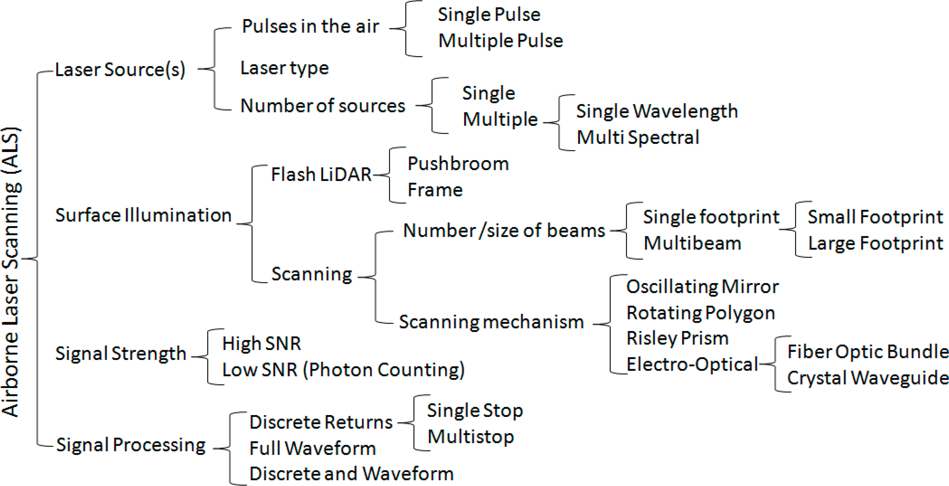
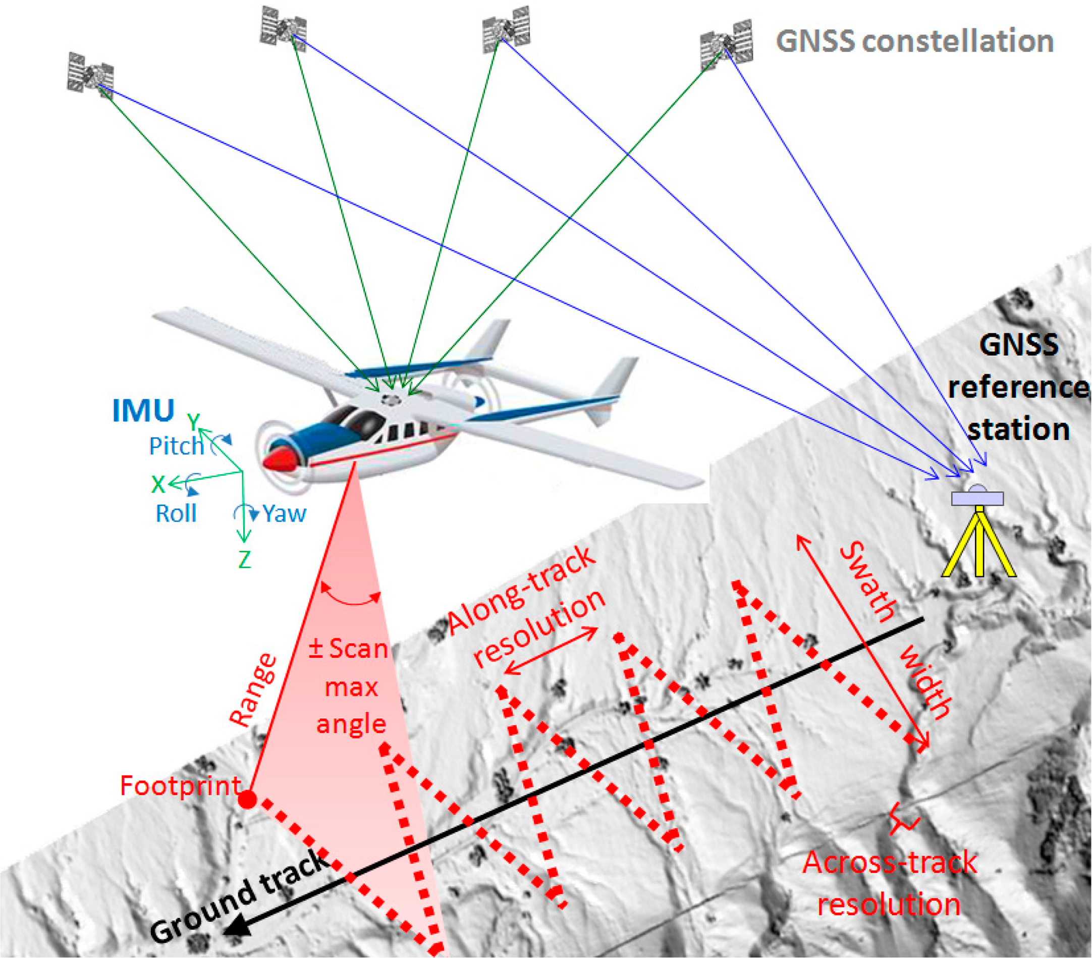
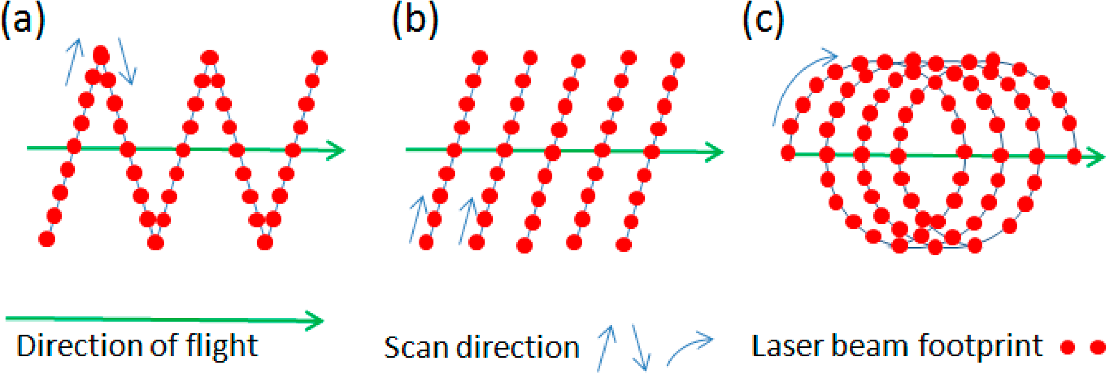
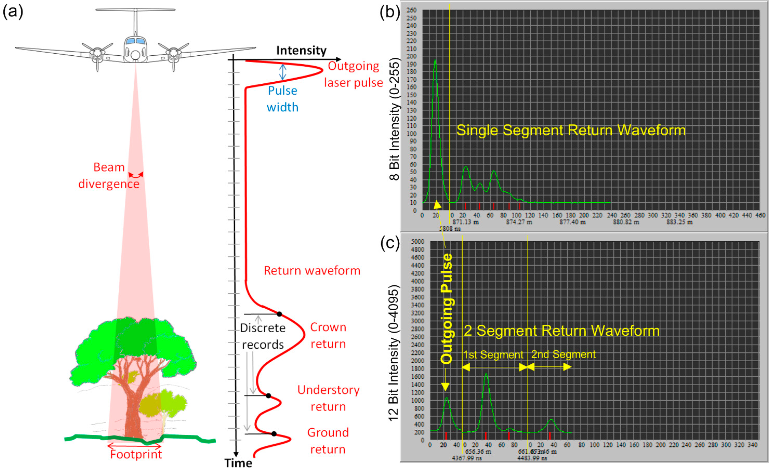
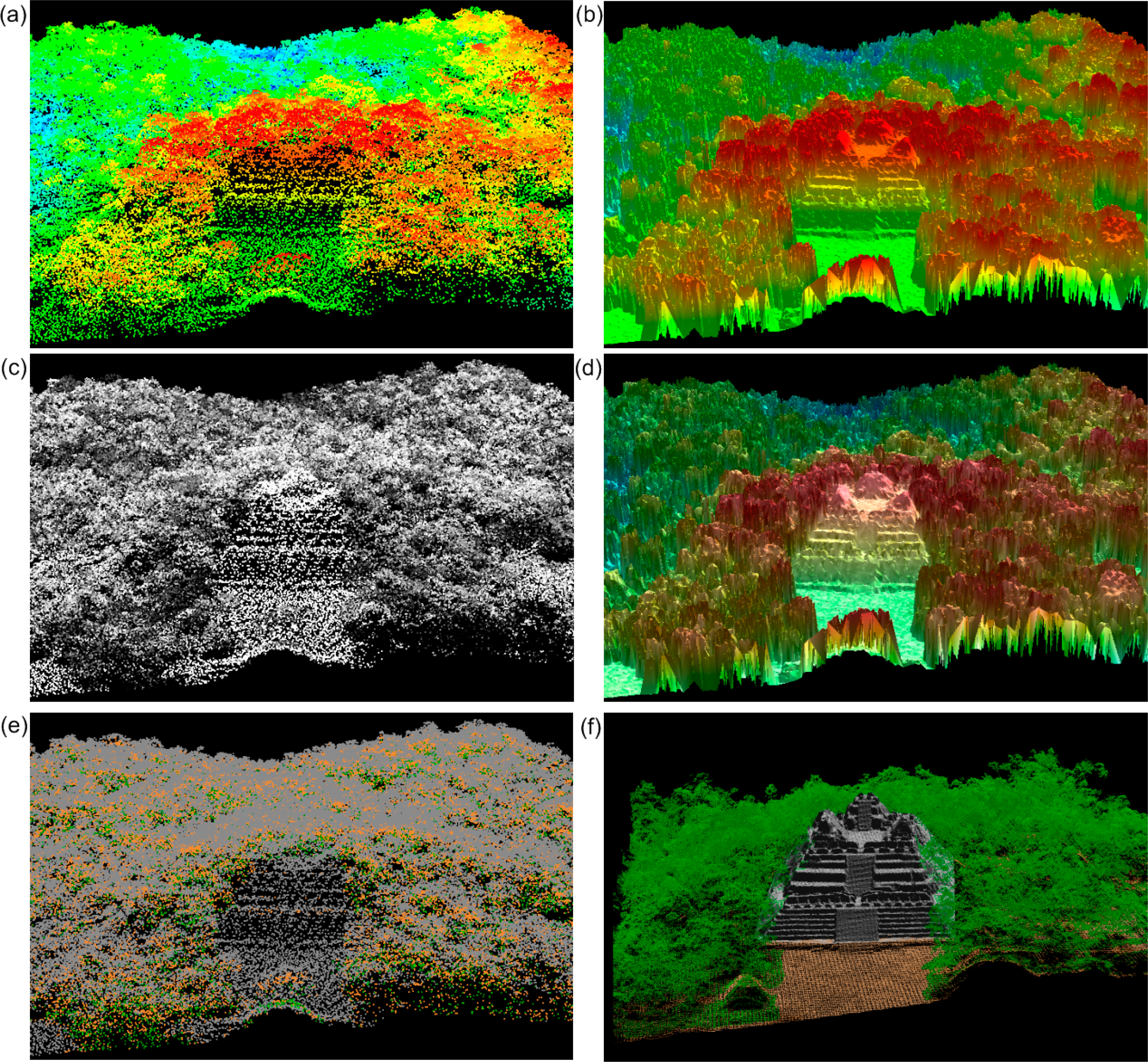
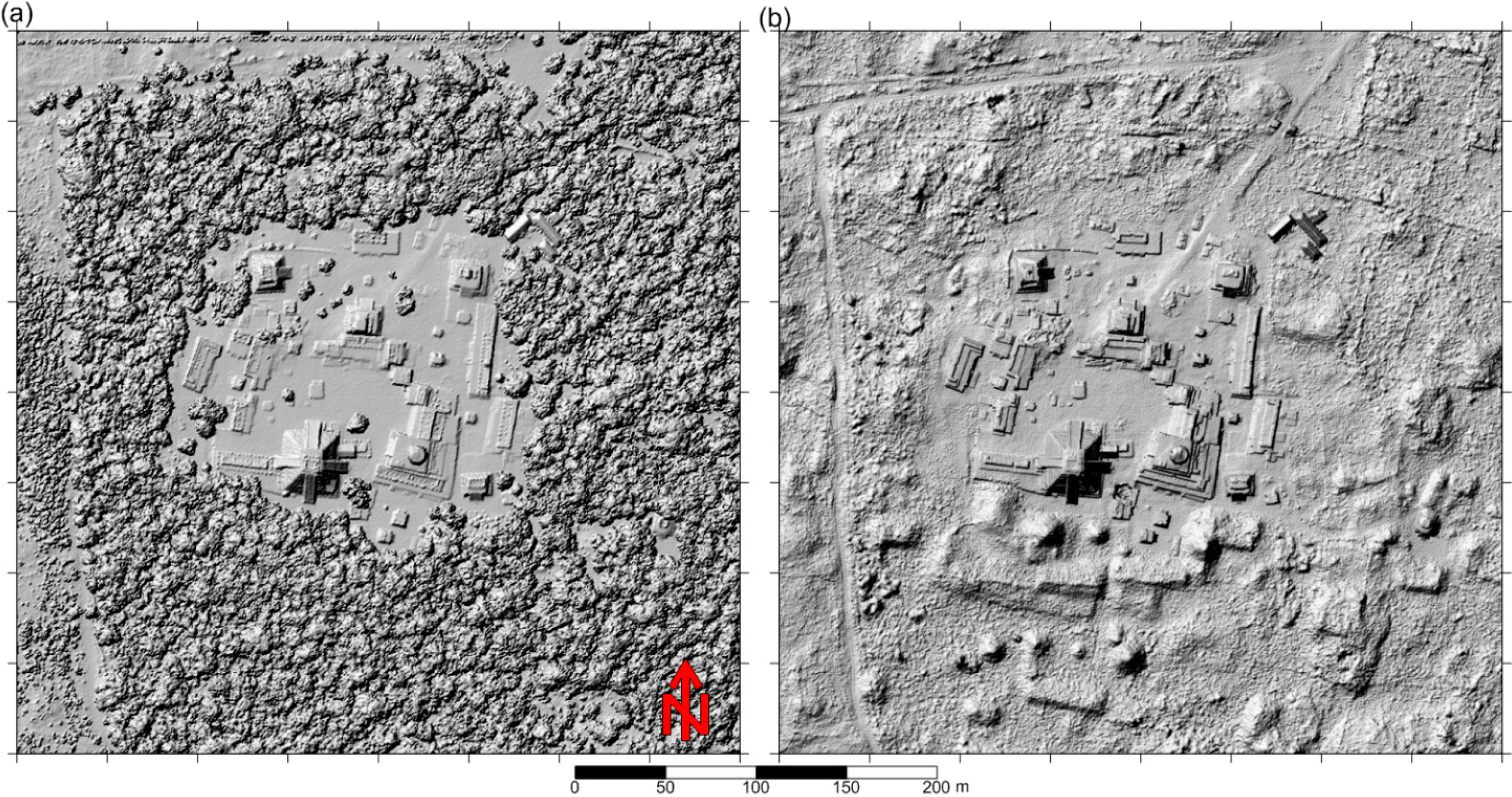
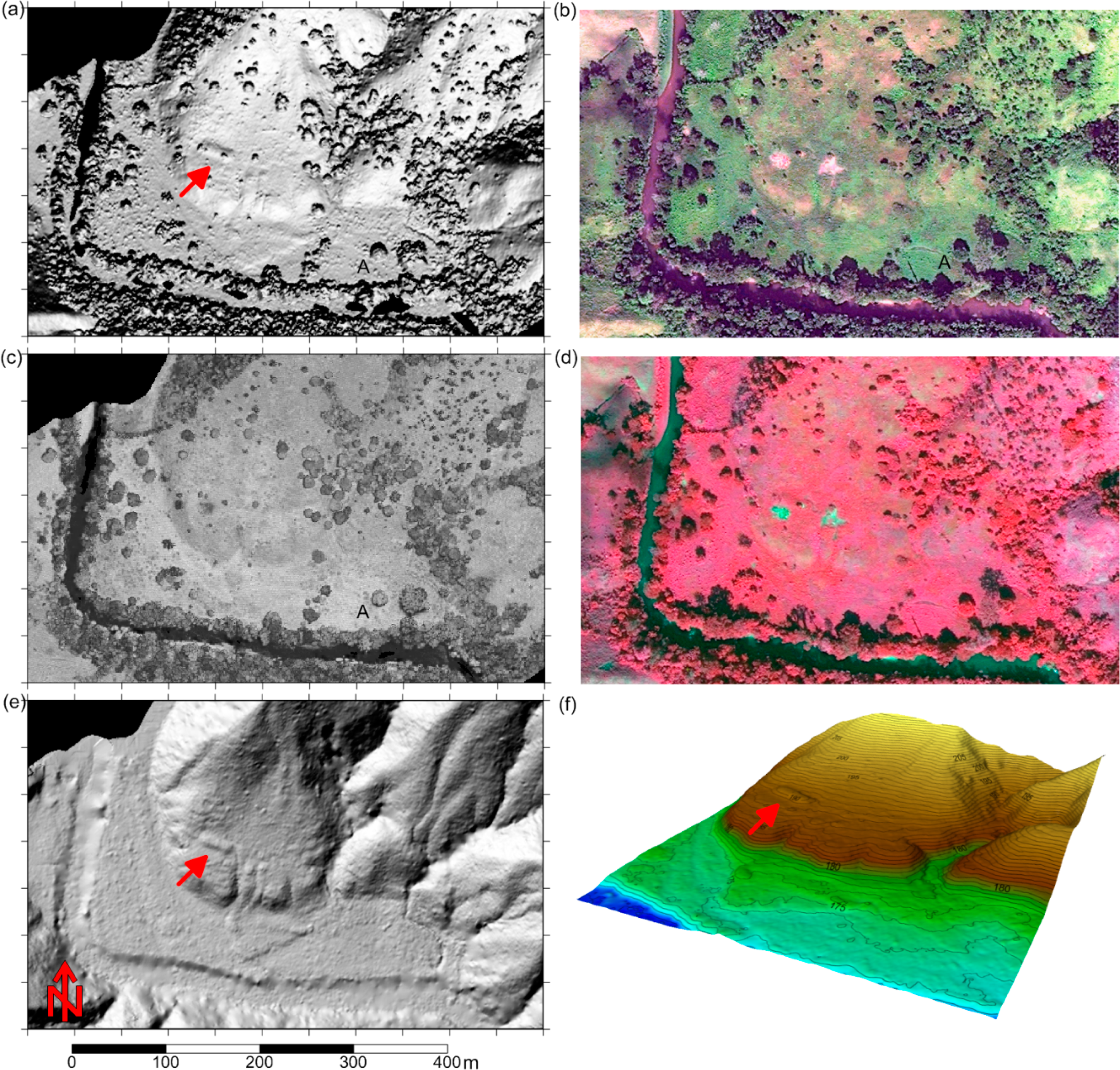
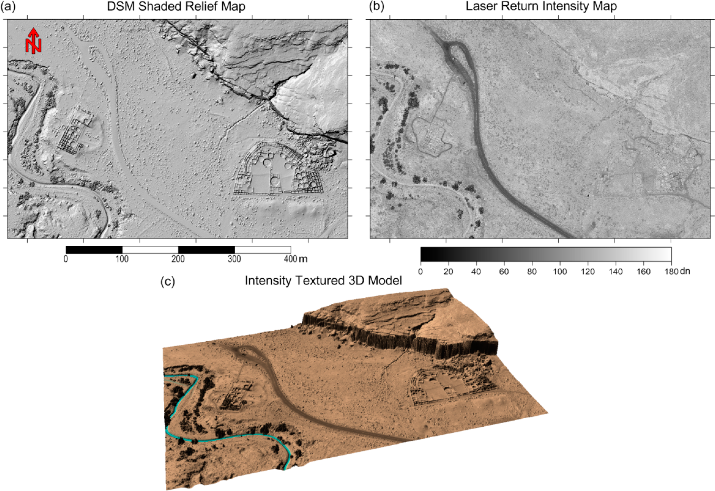
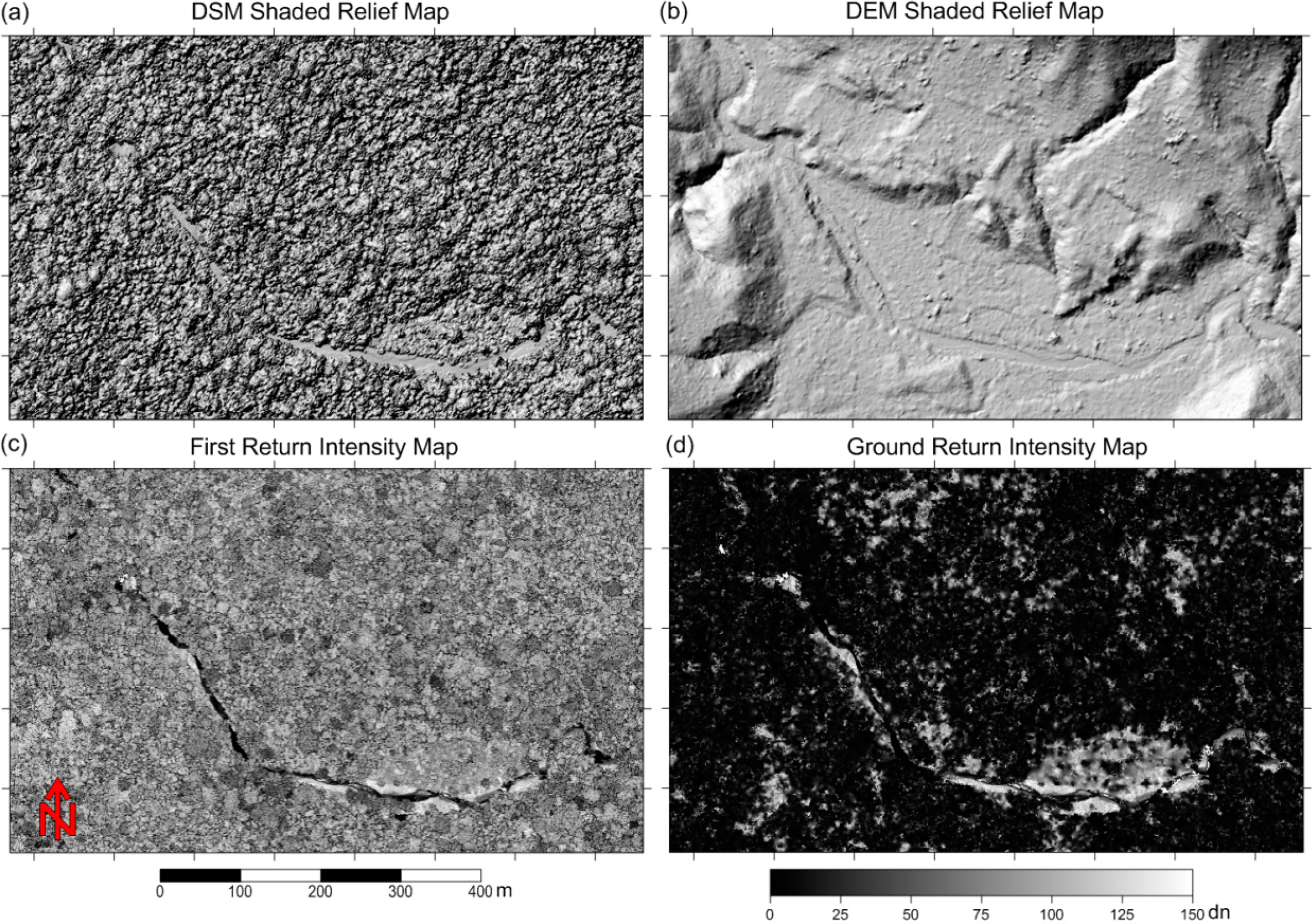
| Project | Survey Year | Area (km2) | Laser Shot Density (s/m2) |
|---|---|---|---|
| Perry Mesa Region, Arizona | 2008 | 40 | 4 |
| Caracol, Belize | 2009 | 194 | 20 |
| Chaco Canyon, New Mexico | 2010 | 40 | 5 |
| Uxbenka, Belize | 2011 | 103 | 12 |
| Mosquitia, Honduras | 2012 | 122 | 15–25 |
| Western Belize | 2013 | 1050 | 15 |
| Mayapan, Mexico | 2013 | 55 | 40–42 |
| Tres Zapotes, Mexico | 2014 | 72 | 12–13 |
| Chichen Itza & Yaxunah, Mexico | 2014 | 50 | 15 |
| Cansahcab, Mexico | 2014 | 26 | 15 |
| Yaxnohcah, Mexico | 2014 | 90 | 15 |
| Configuration | Rtr/Shot | Grn/Sht | Grn/Rtr | Shot/m2 | Rtr/m2 | GR/m2 |
|---|---|---|---|---|---|---|
| Cansahcab, Mexico | ||||||
| 70 kHz 20° × 45 Hz 0.8 mrad | 1.74 | 35.7% | 20.5% | 4.41 | 7.68 | 1.58 |
| 125 kHz 20° × 45 Hz 0.8 mrad | 1.45 | 16.1% | 11.0% | 7.92 | 11.53 | 1.27 |
| Mayapan, Mexico | ||||||
| 100 kHz 20° × 45 Hz 0.8 mrad | 1.59 | 37.0% | 23.3% | 2.98 | 4.74 | 1.10 |
| 100 kHz 20° × 45 Hz 0.25 mrad | 1.48 | 29.7% | 20.1% | 3.33 | 4.94 | 0.99 |
| Calakmul, Mexico | ||||||
| 70 kHz 20° × 45 Hz 0.8 mrad | 1.98 | 26.9% | 13.6% | 2.59 | 5.13 | 0.70 |
| 100 kHz 20° × 45 Hz 0.8 mrad | 1.70 | 16.0% | 9.4% | 3.64 | 6.22 | 0.58 |
| 125 kHz 20° × 45 Hz 0.8 mrad | 1.53 | 9.4% | 6.1% | 6.19 | 9.52 | 0.58 |
| Yaxnohcah, Mexico | ||||||
| 100 kHz 20° × 45 Hz 0.8 mrad | 1.71 | 17.2% | 10.0% | 3.77 | 6.47 | 0.65 |
| 125 kHz 20° × 45 Hz 0.8 mrad | 1.47 | 10.2% | 6.9% | 4.33 | 6.41 | 0.44 |
| Uxbenka, Belize | ||||||
| 50 kHz 20° × 35 Hz 0.8 mrad | 1.74 | 9.0% | 5.2% | 2.01 | 3.50 | 0.18 |
| 125 kHz 18° × 55 Hz 0.8 mrad | 1.26 | 3.5% | 2.8% | 4.01 | 5.06 | 0.14 |
| Mosquitia, Honduras | ||||||
| 125 kHz 15° × 60 Hz 0.8 mrad | 1.65 | 2.7% | 1.6% | 5.90 | 9.79 | 0.16 |
| 125 kHz 15° × 60 Hz 0.25 mrad | 1.47 | 2.3% | 1.6% | 6.00 | 8.86 | 0.14 |
| 142 kHz 15° × 60 Hz 0.8 mrad | 1.45 | 1.7% | 1.1% | 6.96 | 10.10 | 0.12 |
| Method | Exact/Smooth Interpolator | Weighting Method | Allows for Extrapolation |
|---|---|---|---|
| Triangulation Linear Interpolation | Exact | None | No |
| Nearest Neighbor | Assigned | None | No |
| Natural Neighbor | Smooth | Area | No |
| Moving Average | Smooth | None | Yes |
| Local Polynomial | Smooth | Least Squares | Yes |
| Minimum Curvature | Smooth | None | Yes |
| Inverse Distance to a Power | Smooth/Exact | Distance | Yes |
| Kriging | Smooth/Exact | Variogram [58] | Yes |
© 2014 by the authors; licensee MDPI, Basel, Switzerland This article is an open access article distributed under the terms and conditions of the Creative Commons Attribution license (http://creativecommons.org/licenses/by/4.0/).
Share and Cite
Fernandez-Diaz, J.C.; Carter, W.E.; Shrestha, R.L.; Glennie, C.L. Now You See It… Now You Don’t: Understanding Airborne Mapping LiDAR Collection and Data Product Generation for Archaeological Research in Mesoamerica. Remote Sens. 2014, 6, 9951-10001. https://doi.org/10.3390/rs6109951
Fernandez-Diaz JC, Carter WE, Shrestha RL, Glennie CL. Now You See It… Now You Don’t: Understanding Airborne Mapping LiDAR Collection and Data Product Generation for Archaeological Research in Mesoamerica. Remote Sensing. 2014; 6(10):9951-10001. https://doi.org/10.3390/rs6109951
Chicago/Turabian StyleFernandez-Diaz, Juan Carlos, William E. Carter, Ramesh L. Shrestha, and Craig L. Glennie. 2014. "Now You See It… Now You Don’t: Understanding Airborne Mapping LiDAR Collection and Data Product Generation for Archaeological Research in Mesoamerica" Remote Sensing 6, no. 10: 9951-10001. https://doi.org/10.3390/rs6109951