A Life-Size and Near Real-Time Test of Irrigation Scheduling with a Sentinel-2 Like Time Series (SPOT4-Take5) in Morocco

Abstract

This paper describes the setting and results of a real-time experiment of irrigation scheduling by a time series of optical satellite images under real conditions, which was carried out on durum wheat in the Haouz plain (Marrakech, Morocco), during the 2012/13 agricultural season. For the purpose of this experiment, the irrigation of a reference plot was driven by the farmer according to, mainly empirical, irrigation scheduling while test plot irrigations were being managed following the FAO-56 method, driven by remote sensing. Images were issued from the SPOT4 (Take5) data set, which aimed at delivering image time series at a decametric resolution with less than five-day satellite overpass similar to the time series ESA Sentinel-2 satellites will produce in the coming years. With a Root Mean Square Error (RMSE) of 0.91mm per day, the comparison between daily actual evapotranspiration measured by eddy-covariance and the simulated one is satisfactory, but even better at a five-day integration (0.59mm per day). Finally, despite a chaotic beginning of the experiment—the experimental plot had not been irrigated to get rid of a slaking crust, which prevented good emergence—our plot caught up and yielded almost the same grain crop with 14% less irrigation water. This experiment opens up interesting opportunities for operational scheduling of flooding irrigation sectors that dominate in the semi-arid Mediterranean area.

1. Introduction

In the southern Mediterranean region, as well as in other arid and semi-arid areas in the world, water withdrawals have significantly increased over the last decades [1]. In Africa, 12.5 million hectares out of the 210 hectares grown are under fully- or partly-controlled irrigation (about 6% of croplands) according to [2]. In the southern Mediterranean region, this relatively small surface absorbs 86% of water withdrawals. Localized irrigation, like drip irrigation or micro-sprinkler, represents less than 5% of all irrigated areas, while surface and sprinkler irrigations account for 78% and 17%, respectively. Although the move to drip irrigation is strongly encouraged through subsidies in several countries, flooding and sprinkler will certainly remain the dominant techniques in the future, like in Europe [3], but will eventually shift to more sprinkler as pressurized systems appear.

In the arid and semi-arid areas, where water is one of the most limiting factors to the improvement of agricultural production [4], the challenge is to increase agricultural production with limited water resources, thus by improving irrigation management for a more efficient and productive use of irrigation water. Furthermore, the southern Mediterranean region is pointed out as a hotspot of climate change [5] and the part of water allowed to agriculture will be reduced from 90% in 1995 down to 70% by 2020 [6]. Also, in Africa, crop development may be sub-optimal because of nitrogen stress [7,8].

According to [9], irrigation scheduling is the decision-making process of the farmer related to “when” to irrigate and “how much” water to apply to a crop but, as Pereira noticed, “research has made available a large number of irrigation scheduling tools including procedures to compute crop water requirement, to simulate soil water balance, to estimate the impact of water deficits on yields, and to simulate the economic returns of irrigation. However, irrigation scheduling is not yet utilized by the majority of farmers”.

A sophisticated, yet easy to use, assessment of crop development and advice for irrigation scheduling could, then be an interesting tool both at the farming and district scales, especially in a context of surface or sprinkler irrigation and under-optimal crop because of water and/or nitrogen stress. Spatial remote sensing imagery can help to fill the gap between research and implementation of irrigation scheduling.

Depending on the wavelength of the sensor acquiring Remote Sensing Imagery, different biophysical variables may be derived [10]. Several vegetation indices have been made up (SAVI, EVI, etc.) [11], but the Normalized Difference Vegetation Index (NDVI) is considered a common denominator amongst several satellite sensors. Other parameters can also be successfully retrieved from visible remote sensing like the Leaf Area Index (LAI), the Fraction Cover ($f_c$) and albedo.

Several reviews of current modeling of Evapotranspiration and Water Balance with Remote Sensing imagery are available [12,13,14,15,16,17]. They agreed to group methods into four main classes of increasing complexity: (1) empirical direct methods whereby a relationship links Net Radiation to the difference of Air and Surface Temperature; (2) vegetation indices or inference methods, whereby a crop coefficient inferred from remote sensing modulates a Reference Evapotranspiration locally measured; (3) the Residual Method of Surface Energy Balance combines empirical relationships to physical models in order to assess the energy budget components, minus the latent Heat Flux which is determined as the residue of the other fluxes; and (4) the mechanistic approach based on so called Soil Vegetation Atmosphere Transfer models, whereby all the components of the energy and water budgets are computed.

In this experiment, the second method is used with the FAO-56 dual-crop method under water stress conditions described in [18] and its extension [19]. The crop coefficients and fraction covers are inferred from a high temporal and spatial resolution data set acquired and processed in near real-time (a couple of days). To achieve this, the experiment relied on the SPOT4 (Take5) experiment [20] which aimed to provide a Sentinel-2 like data set from February to June 2013. In fact, the two Sentinel-2 satellites will provide high-resolution images of all land areas, every fifth day. This experiment also benefited from the low cloud cover observed in semi-arid areas, which enabled getting a high frequency of cloud-free acquisitions.

This experiment was not carried out in a fully-controlled experimental environment, but on the contrary, on a plot located within an irrigation scheme running as usual. As the scheme distributes irrigation water arranged by rotational turns, the main constraint is then to anticipate the irrigation event at least three days in advance. Such a system is also subject to various contingencies like element ruptures for example. Hopefully, the only contingency during the experiment was a three-day closure of all irrigation events for accounting and recovery of payments. To resolve the timing constraints, the data were gathered in this way: meteorological data from our local station were sent by telemetry, irrigation data from the Agricultural Office were communicated through phone calls, and images through the Internet.

This paper is organized as follows. In Section 2, we provide a description of the study area, the in-situ measurements and satellite imagery, and the specialized FAO-56 method. Section 3 presents the results of irrigation scheduling by satellite imagery, which was carried out on the durum wheat. Section 4 discusses the strengths and weaknesses of the proposed method, and suggests some perspectives.

2. Data and Methods Used

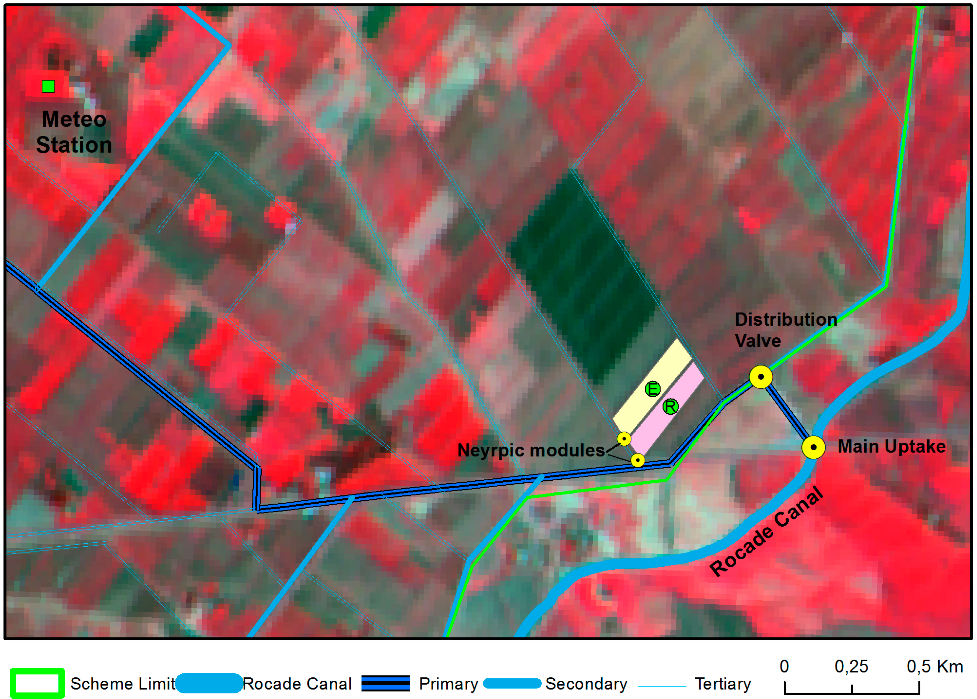
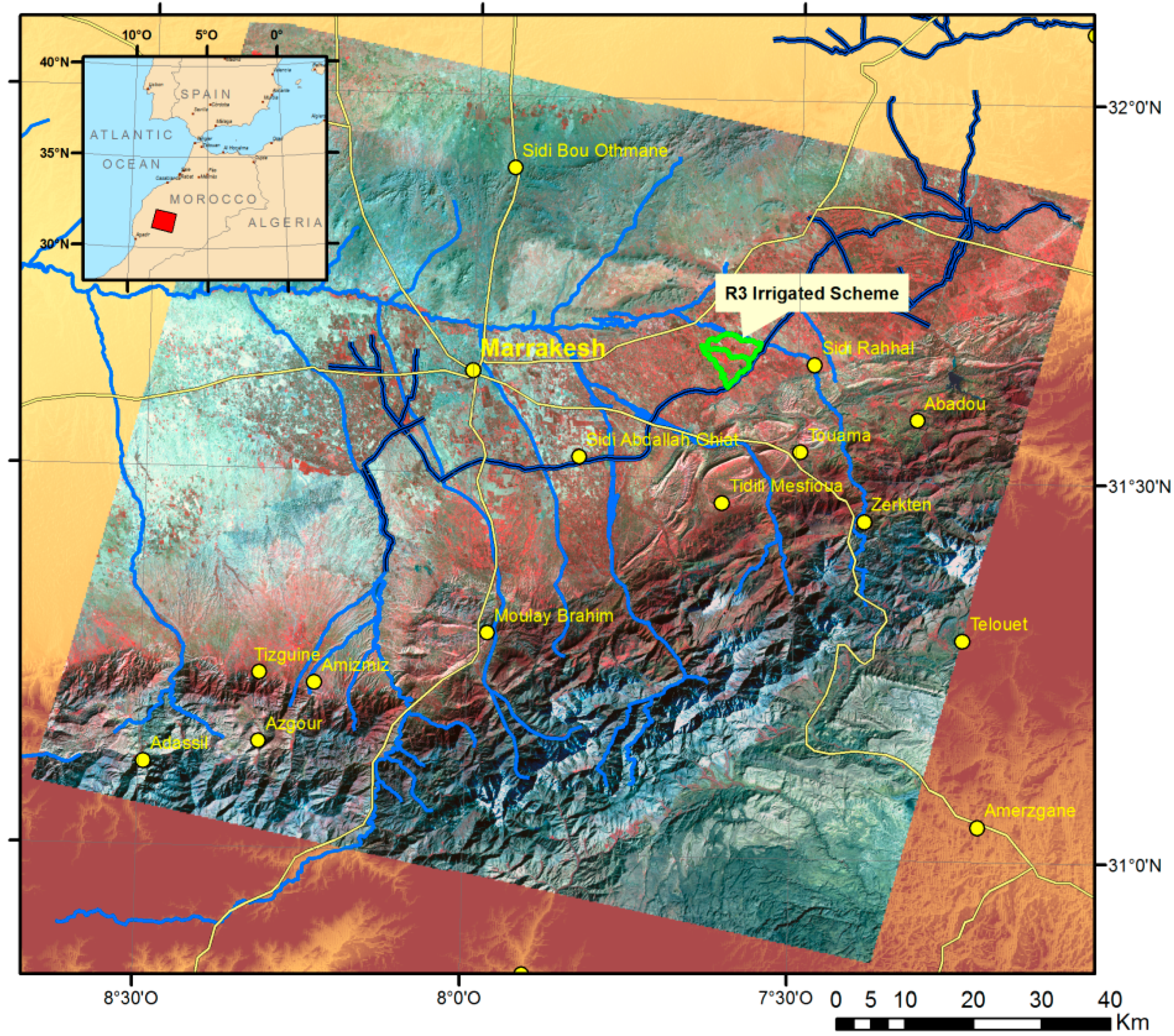
2.1. Study Site and Experimental Plots

The Haouz plain is a sedimentary plain bordered to the North by the Jbilet Mountains and to the South by the High-Atlas Mountains. The plain is crossed from South to North by several wadis, which are the tributaries of two large collectors, the Tensift and Oum er Rbia, which gave their name to their respective watershed.

The plain climate is semi-arid, with average annual rainfall of 250 mm concentrated between November and April, whilst evaporative demand according to the reference evapotranspiration (ET₀) is about 1600 mm per year [21].

The agricultural sector is managed by the Office Régional de Mise en valeur Agricole du Haouz, or ORMVAH. About two thirds of the 473,000 ha of croplands are irrigated, and half of them (144,600 ha) are irrigated from dams.

The experimental plots are located in the R3 irrigation scheme (Figure 1), which encompasses about 3000 ha of irrigated land, composed of about 745 individual fields. R3 scheme is supplied with water from the Hassan dam through the Rocade main canal, which also provides other irrigated areas and the drinking water of Marrakech City. Irrigation water is supplied to the fields via open primary, secondary and tertiary concrete canals that are well-maintained. Neyrpic modules à masque—undershot gate devices—provide control of flow rates by ±5% [22]. According to [22], the allocation of water is determined in three steps. Initially, the seasonal distribution of water is negotiated between the major water stakeholders depending on the availability of water in reservoirs. At the beginning of the irrigation season, the Water User Associations (WUA) are informed about the seasonal water allocated to their sector. A second negotiation phase between WUAs and ORMVAH leads to the monthly and seasonal requirements according to the expected cropping patterns. Thus, the number of irrigation cycles and water depths is fixed in proportion to farm size. During the season, the WUAs adjust the irrigation scheduling by choosing the start date of each irrigation cycle, usually based on simple observations of weather or by visual assessment of crop and soil water status.

Figure 1. The picture shows the area covered with the SPOT4-Take5 images (background is the first image of the Time Series taken on 31 January 2013), and the location of R3 scheme (green), 40 km east of Marrakech, Morocco. The scheme is fed by the Rocade Canal (dark blue).

Figure 1. The picture shows the area covered with the SPOT4-Take5 images (background is the first image of the Time Series taken on 31 January 2013), and the location of R3 scheme (green), 40 km east of Marrakech, Morocco. The scheme is fed by the Rocade Canal (dark blue).

The dominant soil-type is xerosol, developed on colluvial materials of the High Atlas mountains, resulting in homogeneous deep soils (generally more than 1 m), with fine clay to loamy texture. The main crops are cereals (mostly wheat) adding up to 80% of the area on average, the remaining area being planted in olive trees or covered by fallows and villages [22].

Figure 2. Setup at the south of the scheme: The experimental plot (yellow) is located north of the reference plot (pink) at a distance of about 1km from the main canal. A flux tower (green circle) was installed at the center of each plot (E stands for “experimental”, and R, for “Reference”). The meteorological station (green square) is located 2 km west of the plots.

Figure 2. Setup at the south of the scheme: The experimental plot (yellow) is located north of the reference plot (pink) at a distance of about 1km from the main canal. A flux tower (green circle) was installed at the center of each plot (E stands for “experimental”, and R, for “Reference”). The meteorological station (green square) is located 2 km west of the plots.

Two plots were selected at the proximity of a primary canal head (Figure 2) in order not to disrupt the scheduling of the irrigation scheme and to ensure water availability to the experiment. The first plot, hereafter “experimental”, covers an area of 3.7 hectares and irrigation was driven by our model. The second plot (3.3 hectares) is irrigated “as usual” by the farmer, and it is hereafter referred to as “reference”. The four soil samplings conducted at 20 cm and 40 cm depth showed a texture of 36% clay and 20% sand. The pedotransfer function [23] is taken from [24] to obtain a field capacity of 0.32 m³/m³ and a wilting point of 0.18 m³/m³.

2.2. Technical Itinerary

After a proper soil preparation (deep pre-plowing in the summer and soil refinement), durum wheat (Saragola) was sown on 24 December 2012, at a rate of 200 kg/ha. We will further refer to the dates following sowing as DaS (Date after Sowing). Fertilizer was applied at sowing, consisting of 200 kg/ha of Diammonium Phosphate (DAP), and then at the beginning of the grain-filling phase on DaS 106 with 100 kg/ha of Ammonitrate. Weeds were controlled with specific chemical applications on DaS 51 and 108. Harvest took place on DaS 171 (12 June 2013).

Both plots are surface-irrigated. The irrigation technique is Border Irrigation [25]. This technique is widely used in the so-called Modern Irrigation areas of the Haouz plain where the plots have been leveled. A quaternary channel dug by the farmer orthogonally to the distribution canal allows diverting water flow to each strip of land within the plot. Water then travels down the slope while fully filling the soil, thus preventing the control of applied water for each irrigation event. The total length of each border is equal to the width of the plot (about 100 meters) and the width of the border is about 8 m. It takes about half an hour to irrigate one border with two operators, and about 5 to 6 h per hectare. Nevertheless, as described in [25], this technique may not ensure an adequate filling of the root zone, in particular because of poor land grading, wrong stream size, or stopping the inflow at the wrong time. Also according to [26], in the study area, deep percolation was evaluated between 26% and 31% of water supplied (rainfall and irrigation), depending on the stage of crop development.

Because of the clay soil texture, a slaking crust occurs when soil moisture content is below field capacity. In our case, the two plots were irrigated immediately after sowing to ensure germination. Since there was no rain after this period, a second irrigation was necessary after a few days in order to ease wheat emergence (which was realized for the farmer plot). Unfortunately, due to a misunderstanding with the farmer, the test plot did not receive this second irrigation on time.

Also, previous experiments [7,24] on winter wheat on this irrigation scheme had already shown that rooting depth does not exceed 60 to 80 centimeters with this irrigation technique.

2.3. The Time Series of Remote Sensing Images

This experiment was mainly driven by the use Sentinel-2 like data thanks to the SPOT4 (Take5) experiment [20]. The SPOT4 (Take5) experiment consisted in lowering the altitude of SPOT4 orbit by a few kilometers, putting it on a five-day repeat cycle orbit, in order to be able to observe a limited number of sites every fifth day under constant viewing angles. Therefore, the achieved repetitiveness is the same as the one provided by Sentinel-2 mission with two satellites, and the experiment was aimed at helping users prepare their methods and applications to get ready for Sentinel-2 data availability in 2015.

Finally, 45 sites were chosen, among them the Moroccan site in which resides the Haouz plain (Figure 2), and 28 successive images were acquired every fifth day in 2013, from 31 January to 15 June. Data were processed in near real-time to level 2A using the MultiSensor Atmospheric Correction and Cloud Screening software (MACCS) [27,28]. Level 2A data is ortho-rectified images expressed in surface reflectance after atmospheric correction, provided with a cloud/cloud shadow mask.

In total, 18 scenes (64%) were cloud-free for our two plots. As displayed on Figure 3, there were six gaps: two gaps with one missing image (10 days) and four gaps with two missing images (15 days). As the Take5 experiment started one month after sowing, and the success of orbit altitude change was not assured, a SPOT5 programming was also performed, with one image every fifteenth days from December to April. Like all other satellites of the SPOT family, the SPOT5 has the capability to make off-track pointing. Thus the major time interval between two images was only 25 days. SPOT5 atmospheric corrections were carried out with SMAC [29] using the data of the Saada Photometer, 50 km west of the plots.

Figure 3. Time series of satellite images Spot4-Take5, Spot5 and Landsat8 during the 2012/13 season. Landsat8 scenes were not used during the experiment and are only indicated as reference. The gaps in the SPOT4 series are only due to cloud cover.

Figure 3. Time series of satellite images Spot4-Take5, Spot5 and Landsat8 during the 2012/13 season. Landsat8 scenes were not used during the experiment and are only indicated as reference. The gaps in the SPOT4 series are only due to cloud cover.

The NDVI (Equation (1)) based on red (R) and infra-red (NIR) reflectances was finally calculated for each image and averaged for each plot, eliminating edge pixels. This choice is important. First, the border irrigation technique does not allow modifying the applied quantity of irrigation, resulting in the fact that the plot level is the most adequate scale of management for irrigation. Second, although it is very likely that a variability of soil and irrigation exists within the plot, we believe that we cannot afford such accuracy on an operational level, so the water budget may be inaccurate at the pixel level. Third, the algorithm is simplified and computing time is reduced.

$$\text{NDVI}=\left(NIR-R\right)/\left(NIR+R\right)$$

(1)

2.4. The FAO-56 Method Driven with Remotely Sensed NDVI

The FAO-56 method [18,19] is used to estimate crop water requirements based on the concepts of the reference evapotranspiration ET₀ (defining atmospheric demand), and crop coefficients introduced to regulate demand with regards to the specific response of particular crops. The definition of ET₀ is associated with assumptions on key biophysical variables of the system: leaf LAI, surface resistance, albedo, canopy height. Although several alternative methods may be used to approximate ET₀, the recommended method is the Penman-Monteith equation [30].

In optimal agronomical conditions (no disease, water, salt or nutrient stress), the crop evapotranspiration is called ${\text{ET}}_{\text{c}}$. The crop coefficient ${\text{K}}_{\text{c}}$ is the intermediary between ET₀ and ET_c; it takes into account the physical and physiological differences between reference and studied crops. ${\text{ET}}_{\text{c adj}}$ is the evapotranspiration under non-standard conditions Equation (2). In our study, we only deal with water stress introducing the stress coefficient ${\text{K}}_{\text{s}}$ varying from 0 to 1:

$${\text{ET}}_{\text{c adj}}=K_s\times {\text{ET}}_{\text{c}}=K_s\times {\text{K}}_{\text{c}}\times {\text{ET}}_0$$

(2)

The “Dual Crop Coefficient” approach includes a soil water budget module. This is a procedure to predict the impact of specific wetting events that is better suited for irrigation management at the plot scale. The crop coefficient is split into a basal crop coefficient (${\text{K}}_{\text{cb}}$) for crop transpiration and a soil coefficient ${\text{K}}_{\text{e}}$ for evaporation as in Equation (3) [18].

$${\text{ET}}_{\text{c adj}}=\left(K_s\times {\text{K}}_{\text{cb}}+K_e\right)\times {\text{ET}}_0$$

(3)

In this main equation, ${\text{K}}_{\text{s}}$ is explicitly separated while the reduction coefficient of evaporation ${\text{K}}_{\text{r}}$ has been previously introduced into ${\text{K}}_{\text{e}}$ Equation (4):

$$K_e=\min \left[{\text{K}}_{\text{r}}\left({\text{K}}_{\text{c max}}-{\text{K}}_{\text{cb}}\right);{\text{f}}_{\text{ew}}\times {\text{K}}_{\text{c max}}\right]$$

(4)

where ${\text{K}}_{\text{c max}}$ reflects the natural constraints of available energy. It is the upper limit of evapotranspiration for every cropped surface and ranges from 1.05 to 1.3 depending on wind, humidity and crop height. In the spatialized version of the model, a single steady value of 1.15 is used. The fraction of soil that is both exposed and wetted (${\text{f}}_{\text{ew}}$) is equal to 1 for bare soil, and equals to the soil not covered by vegetation (1 − $f_c$) as crop develops.

The review from [31] shows that early works like [32] have found that NDVI was highly correlated with LAI and $f_c$, and that crop coefficient ${\text{K}}_{\text{c}}$ derived from NDVI were independent of time parameters. The study of [33] showed that the basal crop coefficient ${\text{K}}_{\text{cb}}$ can also be derived from a linear relationship of vegetation indices, but pointed out that NDVI saturates at a LAI of about 3.0. The SAVI index [34] that saturates at higher LAI (about 5.0) and that is also less sensitive to changes in soil brightness and moisture is then more appropriate. The linear relationships between $f_c$ and NDVI have shown to be very reliable. For example [35] and [36] found r² > 0.9.

In relatively recent years, progresses have been made on the estimation of the temporal evolution of ${\text{K}}_{\text{c}}$ from remote sensing measurements of vegetation indices (VIs). Some authors have in fact suggested that relationships between crop coefficient and VIs are linear [32], but others have found non-linear relationships [37]. These relationships have been studied for several crops and recently for potato [38], cotton [39], sugar beet [40], maize [41], grapes [42,43] and citrus orchard [44].

For the winter wheat grown in the Haouz plain, we used the relationships established by [24] for NDVI-$f_c$ and [21] for NDVI-${\text{K}}_{\text{cb}}$. They determined the NDVI-${\text{K}}_{\text{cb}}$empirically using eddy-covariance and ET₀ measurements and only keeping the data of unstressed and fully covered days (Equation (5)). The NDVI-$f_c$ relationship was empirically established between fraction cover measured by hemispherical photography and NDVI retrieved with a portable radiometer (Equation (6)). Note that, for the latter, the $NDV{I}_{min}$ parameter has been replaced with a static value of 0.14. Fraction cover has been maintained to its higher value until harvest time;

$${\text{K}}_{\text{cb}}=1.64\times NDVI-0.23$$

(5)

$$f_c=1.18\times NDVI-0.16$$

(6)

A bucket-type water budget is calculated, where a surface bucket is the water source for evaporation, another one for transpiration of the rooting zone and a deeper one for deep infiltration with a simple parameterization to simulate eventual capillary rises. The depth of the evaporative layer is set to 11 cm, with a Readily Evaporable Water threshold set to 10 mm. The second layer varies from 11 to 60 cm at maximum rooting depth in linear relationship to the fraction cover. The total column is set to 150 cm, so that the depth of the third layer is computable by subtracting the second layer.

The Total Water Storage Capacity (TAW) of each layer is the one between field capacity and wilting point (0.32 m³/m³ and 0.18 m³/m³ respectively as mentioned earlier). For each layer, a threshold $p$separates the readily accessible water (RAW) from the one accessed with difficulty [18]. A threshold of 0.55 for winter wheat is set after Table 22 of FAO-56. After reaching this threshold, the layer in question begins to reduce its water losses to ET. Reduction coefficients ${\text{K}}_{\text{s}}$ and ${\text{K}}_{\text{r}}$ are calculated with the same formalism for the water balance of the root layer and upper layer, respectively: If there is less depletion (Di) than the threshold, there is no reduction and then ${\text{K}}_{\text{s}}$ = 1. If the depletion exceeds the threshold, the stress coefficient is computed as the ratio between available water for the process and the less accessible water (Equation (7)).

$${\text{K}}_{\text{s}}=\frac{TAW-Di}{\left(1-p\right)\times TAW}ifDi>RAW$$

(7)

The rooting depth (Zr) is calculated at each time step with a linear relationship to $f_c$ (Equation (8)) where the Zrmax and Zrmin are the maximum and minimum rooting depth and $f_{c}max$ is the maximum fraction cover of the crop. According to the previous studies mentioned above, Zrmin and Zrmax were set to 0.15 and 0.6 meter respectively

$$Zr=Zrmin+\frac{{\text{f}}_{\text{c}}}{{\text{f}}_{\text{c}}\text{ max}}\times \left(\text{Zrmax}-\text{Zrmin}\right)$$

(8)

Depletion of each layer was updated at the end of each day by subtracting rainfall and irrigation, and adding computed ${\text{ET}}_{\text{c adj}}$ and eventual deep percolation. Capillary rise was set to null for this experiment, and as the plots have been graded with a gentle slope for border irrigation, we assumed that runoff to and from the plot was negligible.

As no significant rainfall had occurred during the previous months, the initial soil water content was set to 15%. The model also implements the partition of wetted area by irrigation or rainfall as described in [19], for which the fraction wet was set to 100%.

2.5. Meteorological Data and In-Situ Measurements

Although ORMVAH is well-equipped with four agro-meteorological stations over the Haouz plain, it was decided to put a full meteorological station equipped with telemetry for two reasons: ORMVAH stations are located more than 40 km away from the study site and meteorological data must be available in near real-time. Conventional climatic data were collected over a site located 2 km away from the experimental plots (square in Figure 2). A 2-meter tower was equipped to measure the air temperature and relative humidity using CS215 from Campbell Sc.; wind speed and direction using a Young 5103 anemometer; incoming solar radiation using an Apogee CS300, and finally rainfall was measured using a tipping bucket automatic rain gauge (ARG100, Campbell Scientific Inc., North Logan, UT, USA). The measured values were aggregated to a 30 min time interval, and then transmitted with a GPRS modem connected from the CR200 data logger.

The station was installed over an alfalfa crop maintained in the range 10–15 cm height during the whole experiment. It was considered appropriate to calculate Reference Evapotranspiration following the Penman-Monteith equation. ET₀ appeared to be consistent with the surrounding stations, corroborating that the surface resistance of this crop was compatible with the reference grass described in the FAO-56 method. A total of 99 mm of rain and 604 mm of ET₀ were recorded during the cropping season (Figure 4). Actual applied irrigation inputs of both plots were provided by ORMVAH, based on the opening time of the irrigation canals. As stated earlier, the flow of water into the plot is well controlled thus the irrigation water depth can easily be inferred.

Two towers were installed in the center of each plot at a height of 2 m (green circle in Figure 2). They provided the elements to calculate the four principal components of energy balance. An Eddy covariance instrument provided high-frequency (20 Hz) measurements of three-dimensional air velocity and temperature (CSAT3, Campbell Scientific Inc.); and synchronous water vapor concentration measured with high-speed hygrometers (KH2O, Campbell Scientific Inc.). Soil fluxes were measured with heat flux plates (HFT3-L, Campbell Scientific Inc.), and finally the four net radiation components were measured with a radiometer (CNR4, Kipp & Zonen, Delft, Netherlands). Data was averaged at a 30 min time interval and checked for energy balance closure with the Bowen ratio method with an r² of 0.85 (slope of 1.1) for the experimental plot and 0.92 (slope of 1.06) for the reference plot. Although not being applied here, it may be noted that other energy balance closure techniques exist. In particular, the study of [45] showed that differences of +10% to −20% of yearly cumulated ET compared to the Bowen Ratio technique may appear. Actual evapotranspiration measured with this system will be further referred to as $E{T}_{EC}$.

Figure 4. Time evolution of Rainfall and Reference Evapotranspiration (ET₀) during the experimental setup.

Figure 4. Time evolution of Rainfall and Reference Evapotranspiration (ET₀) during the experimental setup.

At harvest time, above-ground biomass and grain yield measurements were carried out by counting the total number of straw bales (dry biomass) and the number of grain sacks. Mean plot yields were finally computed by multiplying those accounts by the average weight of sacks and bales obtained through weight sampling.

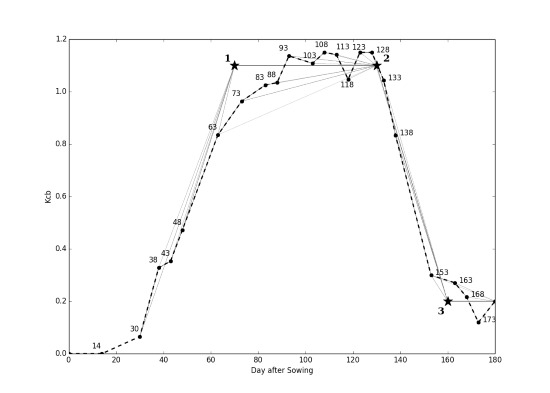
2.6. Kc_b Extrapolation

Changes in NDVI over a five-day period (return period proposed by SPOT 4 (Take 5) or Sentinel 2) are rather small. However, cloud cover increases this interval, and an extrapolation between the latest clear satellite image and the current day is required. Tables 11 and 17 from [18] were used to set up future inflexion points, choosing the California Desert Winter Wheat crop with a cycle length of 160 days. For the FAO-56 approach, the inflexion points are obtained combining the duration of three development stages (initial = 20 days, development = 50 days, mid-season = 60 days and late season = 30 days, for the selected crop), and the basal crop coefficients at initial, mid and late season (0.15, 1.1, 0.25 for the selected crop). The FAO-56 inflexion points were combined with the existing points obtained from remote sensing to calculate a full season by linear interpolation.

2.7. Climatic Extrapolation or Forecast

A forecast of climatic data is needed to help the irrigation decision-making process. The ASP weather model, which is a hybrid-mass coordinate primitive equation hydrostatic model with equations expressed in flux form [46] has been running over the Moroccan domain at 10km resolution during the whole experiment. The rainfall output of the model was scrutinized and compared to freely available model output from the Web. Smallest rain forecasts were simply ignored. Nevertheless, ET₀ forecasts were extracted from climatology because of technical difficulties. We will discuss the importance of these data in the last part of this paper.

2.8. Irrigation Decision-Making Process

As mentioned above, the irrigation scheduling of the reference and the experimental plots were managed separately. The reference plot was managed “as usual” by the farmer, meaning that he had to take not only into account this plot, but also the hundreds of hectares he is growing, and to manage its workforce.

The experimental plot was managed according the FAO-56 method guided by remote sensing NDVI, but taking into account that network management and labor mobilization generally takes a minimum of three days. The triggering of irrigation may thus have been underoptimal in a modeling point of view, as the RAW may not have been fully depleted. It was also decided to let the farmer irrigate by himself the experimental plot before vegetation emergence was noticeable on satellite images (DaS 27 with a NDVI of 0.17), and for the last irrigation.

The irrigation water depths actually applied are dictated by the irrigation technique. They are between 50 and 60 mm.

3. Results

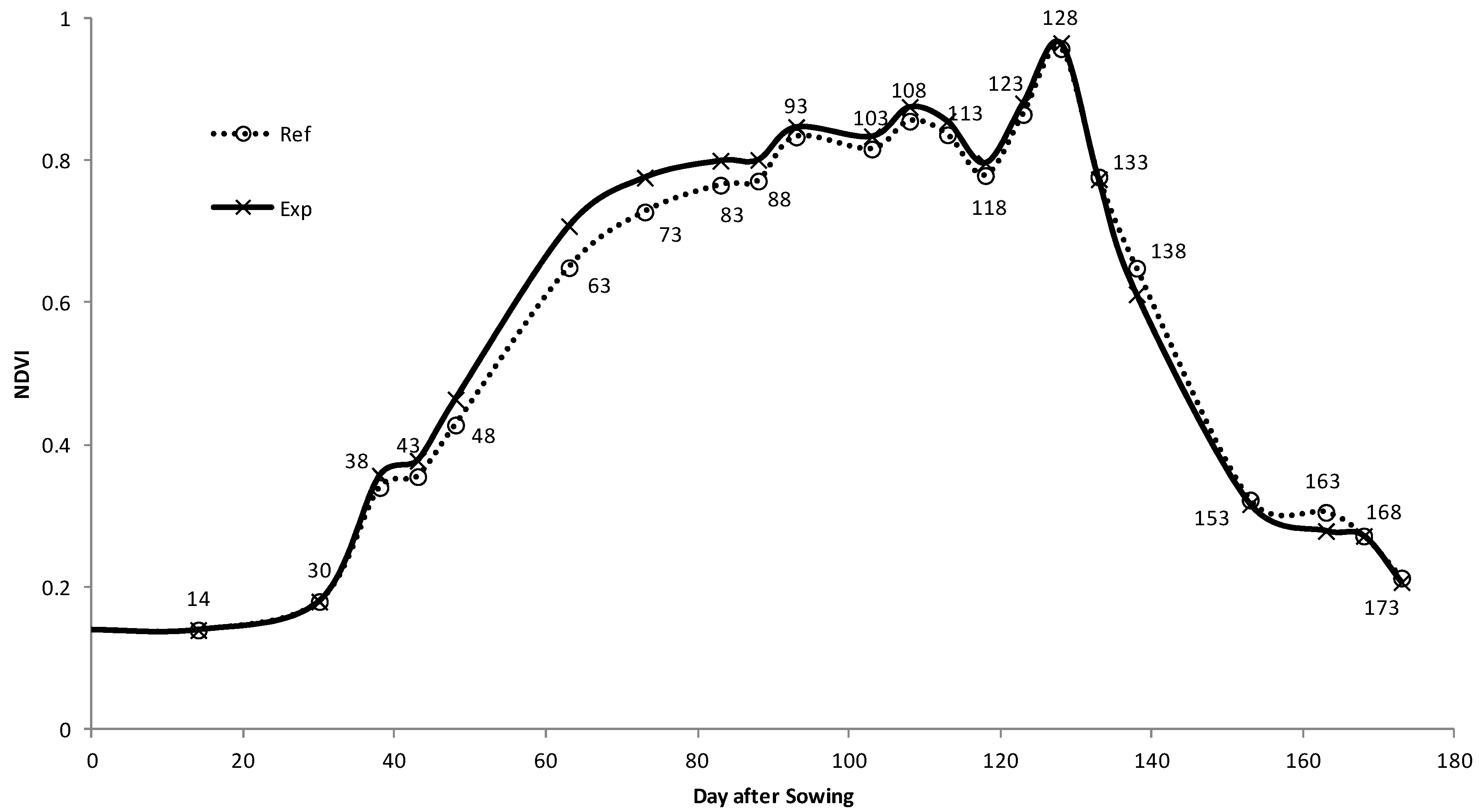
3.1. NDVI and Basal Crop Coefficient

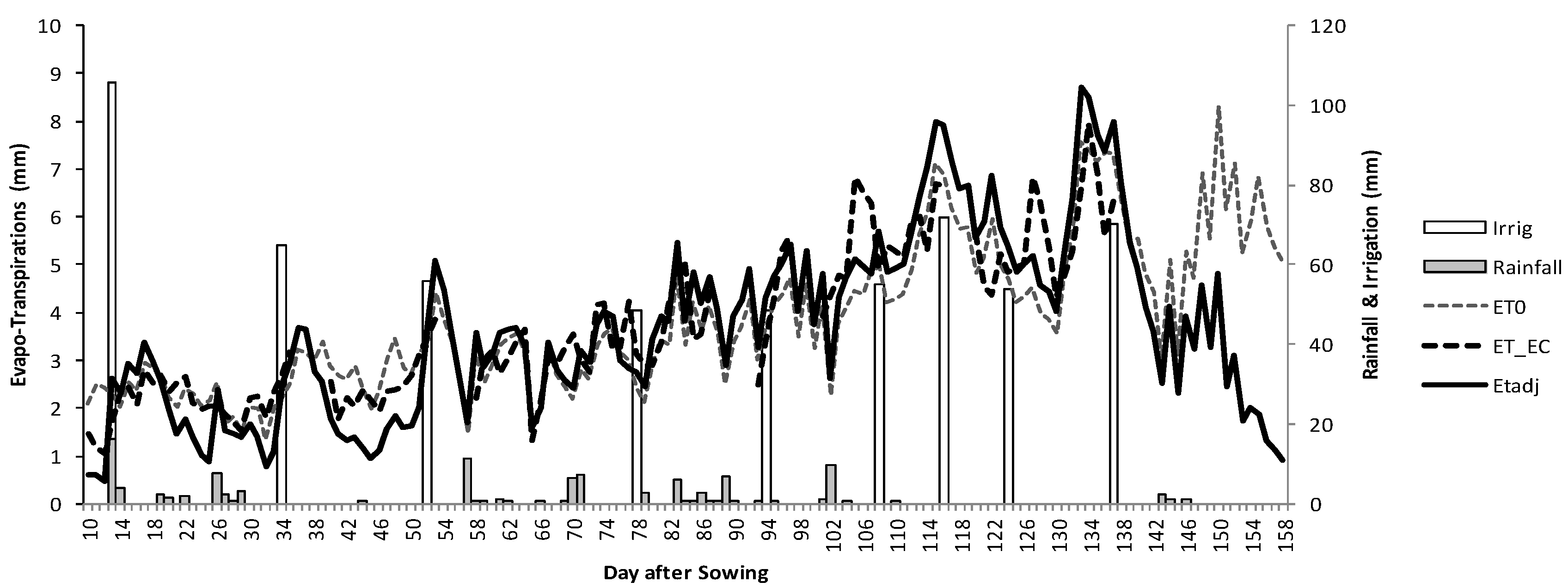
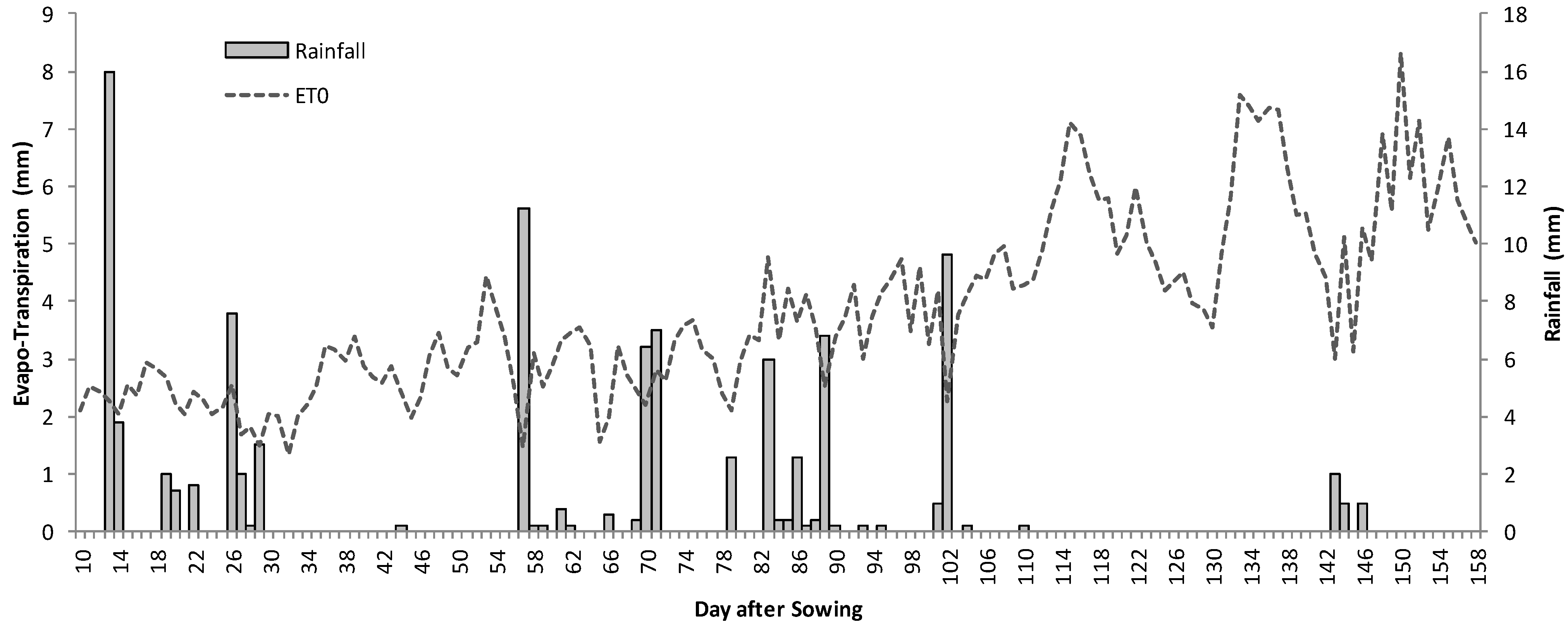
The time series of NDVI for both plots is shown on Figure 5. The first three dates are calculated from SPOT5, the remaining dates are obtained from SPOT4 (Take5). The reference plot shows a lower NDVI during the growth period. The two plots reach the same level of NDVI around DaS 100 (23 March). The jumps in both curves may be related either to soil moisture conditions as wetting events are likely to impact the soil albedo [47], either to a possible increase of aerosols thickness in particular on hot and windy days.

On Figure 6 showing results of the linear conversion from NDVI to Kc_b, it can be seen that Kc_b is limited to Kc_max (1.15), and that the extrapolator was quite efficient. The reception of new images could correct the Kc_b trajectory, especially on DaS 63 when the Kc_b curve began inflecting, and at DaS 133 at the early start of senescence.

3.2. ET Estimates

Figure 7 shows the comparison between $ET{c}_{adj}$ and $E{T}_{\text{EC}}$ for the experimental plot. With RMSE’s of 0.91 mm per day and 0.95 mm per day, and $r^2$ values of 0.75 and 0.67 for the experimental and reference plots, respectively, the comparison shows a fair yet not excellent fit for both fields. These error ranges are quite comparable to previous studies [21,24,48]. The score is particularly low at the beginning of the season, in particular because of lower evaporation during DaS 23–29 and 32–49 (Figure 7). A post-experiment calibration procedure showed that the use of the capillary rise equations would have improved the overall RMSE by 0.09 mm per day (0.28 mm per day for the first 40 days), and that a full calibration of $ET{c}_{adj}$ and $E{T}_{\text{EC}}$ would have helped gain an extra 0.07 mm per day. It can also be remembered that Eddy-covariance measurements are prone to a certain amount of error [49]. In addition, an error analysis at a five-day time interval shows RMSE of 0.59 mm per day and $r^2$ of 0.9 (0.46 and 0.91 with corrected diffusion) for the experimental plot. The gain in RMSE obtained by this temporal integration shows that if the technique does not perform very well on a daily time step, the results are improved over a longer period of time. With regards to irrigation, this information may be interpreted in this way: during the colder period of growth (December–February), average ET was 2.4 mm per day, the irrigation scheduling may be shifted up to one day per every five days, while during the warmer period (average ET of 4.8 mm per day), it goes down to one day per every 10 days. It suggests that the estimates of evapotranspiration are enough accurate for the purpose of irrigation scheduling.

Figure 5. Evolution of NDVI for the two plots: Reference (Ref) and Experimental (Exp). Note that the first three points come from SPOT5 and others from SPOT4. The DaS of each input image has been labeled.

Figure 5. Evolution of NDVI for the two plots: Reference (Ref) and Experimental (Exp). Note that the first three points come from SPOT5 and others from SPOT4. The DaS of each input image has been labeled.

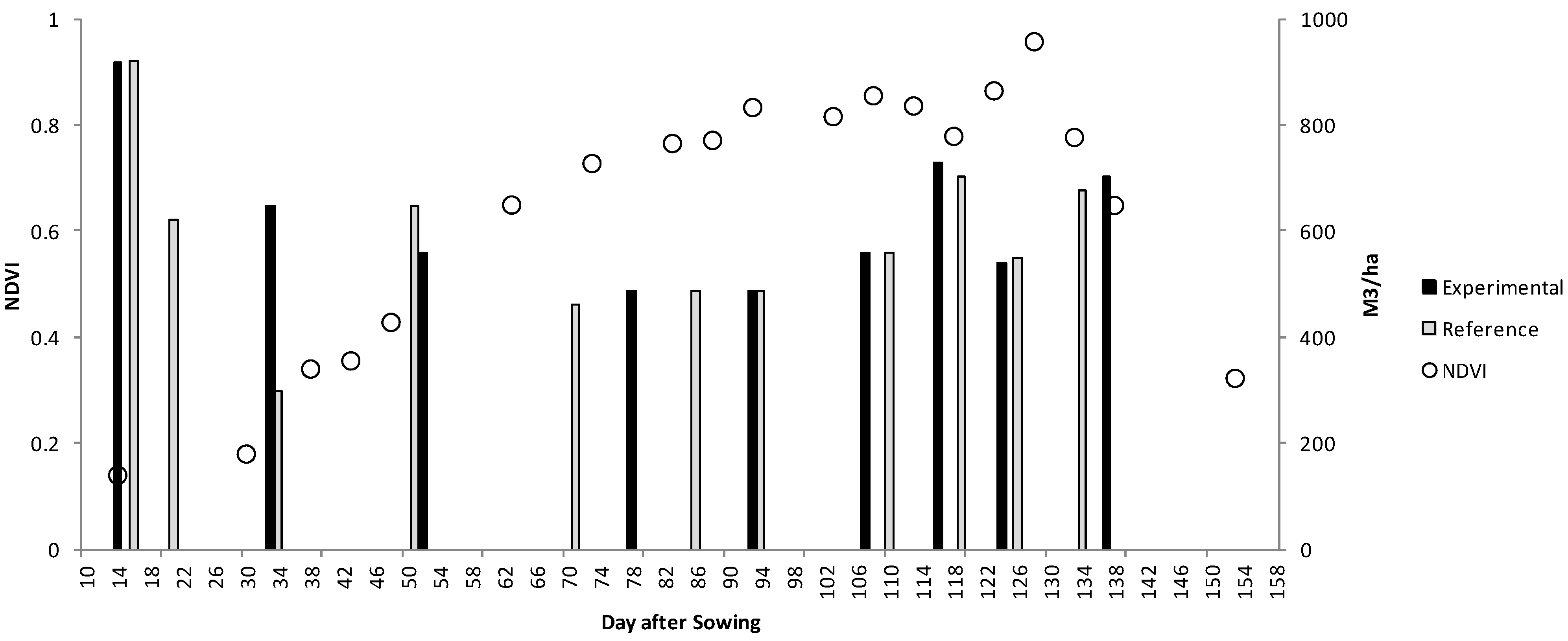
3.3. Irrigation Decisions

As shown on Figure 8 and Figure 9, eleven irrigations events (640.8 mm) were done on the reference and nine on the experimental plot (562.9 mm). They were scheduled fairly differently. As explained earlier, the irrigation decisions were left to the farmer before noticing the emergence of vegetation on NDVI images for both plots.

The farmer decided its first irrigation on DaS 17 with 92 mm (note that a rainfall of 16mm was registered this same day). It is the highest amount in single irrigation during the whole season.

Figure 6. Kc_b derived from NDVI (dashed line) and evolution of extrapolations as new images are arriving (dark to light gray) for the experimental plot. Each time a new image is received (dot and DaS small label), the Kc_b trajectory is corrected. The three inflexion points extracted from the FAO-56 tables are indicated by a star and a bold label.

Figure 6. Kc_b derived from NDVI (dashed line) and evolution of extrapolations as new images are arriving (dark to light gray) for the experimental plot. Each time a new image is received (dot and DaS small label), the Kc_b trajectory is corrected. The three inflexion points extracted from the FAO-56 tables are indicated by a star and a bold label.

Figure 7. Comparison between the daily values of estimated $E{T}_{adj}$ by the FAO-56 model and the measured one $\left(E{T}_{EC}\right)$ by the Eddy-covariance system for the experimental plot. Error indicators are MSE (Mean Square Error), RMSE (Root Mean Square Error), MBE (Mean Bias Error), MAE (Mean Absolute Error) and MAPE (Mean Absolute Percentage Error).

Figure 7. Comparison between the daily values of estimated $E{T}_{adj}$ by the FAO-56 model and the measured one $\left(E{T}_{EC}\right)$ by the Eddy-covariance system for the experimental plot. Error indicators are MSE (Mean Square Error), RMSE (Root Mean Square Error), MBE (Mean Bias Error), MAE (Mean Absolute Error) and MAPE (Mean Absolute Percentage Error).

Figure 8. Forcing (ET₀, Rainfall and Irrigation) of the Water Balance and comparison of measured Evapotranspiration (ET_EC) and Calculated Evapotranspiration (ETadj) for the experimental plot.

Figure 8. Forcing (ET₀, Rainfall and Irrigation) of the Water Balance and comparison of measured Evapotranspiration (ET_EC) and Calculated Evapotranspiration (ETadj) for the experimental plot.

Figure 9. Comparison of irrigation events between the two plots. Time intervals between events are indicated in the same figure. NDVI is for the experimental plot.

Figure 9. Comparison of irrigation events between the two plots. Time intervals between events are indicated in the same figure. NDVI is for the experimental plot.

The farmer decided a second irrigation on DaS 22 and before plant emergence to prevent the appearance of soil crusting. As our water balance model is only efficient after the emergence of the crop, both plots should have been watered the same way. But, although there was no plant emergence, misunderstandings with the farmer led him not to irrigate the experimental plot simultaneously with the reference one. Unfortunately, the soil crust actually appeared on the experimental plot and imperiled the wheat development for the rest of the season (see discussion below), by limiting the number of tiller.

The two following irrigations were done at the same time on DaS 34 and 52.

The next irrigation schedule was significantly different. Indeed, the farmer decided to irrigate on DaS 71, while the experimental plot had been irrigated a week later (DaS 79). It may be noticed that the changing rainfall forecast had moved the date of this irrigation from DaS 75 to 79, and that subsequent measurement of rain and ET₀ showed that this irrigation could have been delayed until DaS 81.

The farmer did irrigate on DaS 87 as well. The next irrigation was carried out on the same day (DaS 94 and 95). For the next irrigation, the farmer waited three more days than we did. It is possible that the farmer had overestimated the amount of rain on DaS 101–103.

The third remaining irrigation events were quite similar in terms of quantity and timing of each plot, but with a three-day interval. The decision to make the last irrigation for both plots was left to the farmer.

3.4. Final Budget and Yields

At the end of the experiment, the final irrigation budget of the experimental plot (563 m³/ha) is lower than the reference plot (640.8 m³/ha). The biomass of the reference plot is 24% higher than the experimental plot and the grain yield is slightly higher (+6% for the reference plot). The almost 14% of extra water used on the reference plot is due to the fact that the farmer used the remaining of irrigation of DaS34 to irrigate its plot and that he did an unnecessary irrigation during the period of Das 71–94.

Table 1. Actual irrigation events of both plots and comparison of irrigation events three to eight to the water balance.

Reference			Experimental
#	Dates (DaS)	Quantity (mm)	#	Dates (DaS)	Quantity (mm)	Water Balance	Absolute Difference (WB-Exp)	Percentage (WB-Exp)
1	9 January (17)	92	1	7 January (14)	91.8	-	-	-
2	14 January (22)	62.1	-	-	-	-	-	-
3	26 January (34)	30	2	26 January (34)	64.8	-	-	-
4	13 February (52)	64.8	3	14 February (53)	56	38	18	32
5	4 March (71)	46	4	12 March (79)	48.6	56	−7.4	−15
6	20 March (87)	48.6	-	-	-	-	-	-
7	27 March (94)	48.6	5	28 March (95)	48.6	49	-0.4	-1
8	13 April (111)	56	6	10 April (108)	56	53	3	5
9	22 April (120)	70.2	7	19 April (117)	72.9	47	25.9	36
10	29 April (127)	55	8	27 April (125)	54	48.9	5.1	9
11	7 May (134)	67.5	9	10 May (137)	70.2	-	-	-
Total Irrigation		640.8			562.9
Total with Rainfall		739.8			661.9

Table 1. Actual irrigation events of both plots and comparison of irrigation events three to eight to the water balance.

Reference			Experimental
#	Dates (DaS)	Quantity (mm)	#	Dates (DaS)	Quantity (mm)	Water Balance	Absolute Difference (WB-Exp)	Percentage (WB-Exp)
1	9 January (17)	92	1	7 January (14)	91.8	-	-	-
2	14 January (22)	62.1	-	-	-	-	-	-
3	26 January (34)	30	2	26 January (34)	64.8	-	-	-
4	13 February (52)	64.8	3	14 February (53)	56	38	18	32
5	4 March (71)	46	4	12 March (79)	48.6	56	−7.4	−15
6	20 March (87)	48.6	-	-	-	-	-	-
7	27 March (94)	48.6	5	28 March (95)	48.6	49	-0.4	-1
8	13 April (111)	56	6	10 April (108)	56	53	3	5
9	22 April (120)	70.2	7	19 April (117)	72.9	47	25.9	36
10	29 April (127)	55	8	27 April (125)	54	48.9	5.1	9
11	7 May (134)	67.5	9	10 May (137)	70.2	-	-	-
Total Irrigation		640.8			562.9
Total with Rainfall		739.8			661.9

Table 1 shows two things: first, a comparison of quantities applied to both plots and second, a comparison of actually applied quantities for the experimental plot to the quantities recommended by the water balance model (the water needed to fill-up the two upper buckets referring to the surface and the root zones respectively), for irrigation events three to eight. We chose to compare only those events because during the initial phase (no vegetation cover), the irrigation scheduling was handled by the farmer and the decision of the last irrigation was also left to the farmer. The comparison to the water budget shows a surplus of 13% for irrigation events three to eight, so the difference is not too large. Nevertheless, the amount of water applied to the first two irrigations is much more important than the budget proposed water. This difference is directly related to the irrigation technique itself, which requires a minimum amount of water to irrigate the entire field, especially on dry and plowed soils at this time of the year.

4. Discussion and Perspective

4.1. Strengths and Weaknesses

A time series of optical high resolution images, very close to what the Sentinel-2 product will look like, was used to compute a daily water balance in near real-time for a wheat field in Morocco, and irrigation was scheduled according to the model prediction. Calculations were performed at the plot level because it is not possible to irrigate a subpart of the plot and also to cut calculation time. A good knowledge of local parameters (soil and rooting depths), realistic input values of ET₀ and the wetting events and a dense time series of high-resolution remote sensing images allow the FAO-56 model to perform properly. By contrast, with Landsat 8 (launched on 11 February 2013 with the first image of our area available on 19 April and a return period of 16 days), a gap of 47 days (two missing images in a row) occurred between the 5 May and 22 June images (Figure 3). In our case, the high frequency of SPOT4 (Take5) allowed a consistent, high repetitiveness data set.

This simple model provides good advice in the irrigation decision-making process, yet several aspects may affect the water balance. Namely, (a) the farmer’s expertise remains crucial; (b) calibration should be adjustable; (c) extrapolation is important to preclude satellite image gaps; (d) the meteorological forecasting especially for rainfall may also be important, but mainly to make the decision of postponing an irrigation event and (e) a time window for irrigation should be provided to the farmer:

(a)

The FAO-56 method is dedicated to the estimation of evapotranspiration and to assist irrigation scheduling. Anything that falls out of this area must be addressed by the farmer’s expertise. In our case, the appearance of a slaking crust greatly disadvantaged the tillering of the experimental plot, and the crop could never recover. This is the main reason for the much lower biomass obtained on the experimental plot. By contrast, the reference crop may have suffered some stress hampering grain filling, leading to a similar amount of grain yield in both plots. In this case, the water budget guided by remote sensing was more efficient than the farmer’s management.

(b)

Although predefined calibrations may be assigned for typical crops and soil parameters, they should be adjustable by the farmer, so that the model could reflect local measurements (e.g., Watermarks) or his know-how of irrigation scheduling (delaying or advancing irrigation triggering).

(c)

The typical description of crops through crop coefficients includes four inflexion points; hence, it can be assumed that four perfectly-timed images would be sufficient to describe the temporal evolution of the crop. However, at a regional level, the spatial variation of sowing dates is important. It increases this theoretical number to a daily image. In addition, cloud coverage forces the need for extrapolation.

(d)

Although it was not demonstrated here, the prevailing forecast data is the rainfall amount. An expected rainfall of 20 mm may boost the root layer for the next few days. But, if the actual rainfall is much lower than the forecast, an irrigation decision must be made rapidly, and still a couple days ahead of the irrigation event because of the technical constraint at the scheme scale. In semi-arid areas, the irrigation decision system should take into account the uncertainty of rainfall forecast, including ignoring the forecasts of small rainfall.

(e)

In the introduction, we said that an irrigation scheme may suffer contingencies, and it is also clear that a farmer has to deal with his equipment and workforce availability. On the other hand, the FAO-56 model suggests a single best date of irrigation. To overcome the problem, it would be nice to provide an irrigation window to the farmer, which would also take into account the preceding remark.

Interestingly enough, during tillering and stem extension the NDVI of the experimental plot was slightly higher than the reference plot, when actually there were about 20% fewer stems on average. This may be explained by the fact that at higher density of leaves, higher shade occurs within the canopy, thus radiation interception is higher [50]. In fact, due to the limited penetration of the visible signal in the canopy, the three dimensional complexity of a crop canopy can hardly be seen by optical remote sensing imagery; hence NDVI remains a broad indicator of crop development, in particular for biomass.

The soils of the Haouz plain are poor and the climate is semi-arid. The yield depends on irrigation, but above all on fertilization. The water productivity indices in the region are generally low (1.63 m³/kg for 2002/03 and 1.49 m³/kg for 2003/04 [7]. In our study, water productivity is 1.34 m³/kg against 1.52 m³/kg for the reference plot (calculated only on irrigation water), which represents a gain of 0.18 m³/kg. This conclusion goes into the way of increasing water productivity which is one of the main concerns of the National Agricultural Plan of Morocco [51].

4.2. Conclusions and Perspective

This experiment demonstrated how remote sensing time series could be used in an almost operational way for irrigation scheduling at the plot scale in a semi-arid environment. In this particular case, this irrigation advice showed to be a possible way to improve performance while saving on water, even without changing the irrigation technique. High-resolution and high-frequency satellite optical images, like the ones that will be available with Sentinel-2, may be of great help for irrigation scheduling at the plot scale. The simulated Sentinel-2 data set provided by the SPOT4 (Take5) experiment proved to be perfectly fitted for this experiment.

Additionally to high temporal and spatial resolution reflectance images, a better assessment of surface soil moisture and root soil moisture can be achieved through assimilation techniques of high temporal and spatial resolution microwave data on the one hand, and thermal data on the other hand [52]. Active microwave in the L and C bands have proven to be particularly interesting for the estimation of soil moisture in the first centimeters [53] for bare soils. With a revisit time of one to three days and a ground resolution of 5 × 20 m, Sentinel-1 data would be a good candidate to help a reflectance-based crop coefficient approach in the early part of the season. This real-life experiment was carried out over a single plot. Other works show the potentiality of the approach for a whole irrigated sector, introducing a new Irrigation Priority Index [54] and an optimization scheme [55]. But the change of scale is not at all straightforward. Initialization will be difficult, in particular because dealing with a large number of plots would imply to automate several steps like crop detection and its corresponding Kc_b profile for interpolation. At running time, actual irrigations, which is crucial input appears to be extremely difficult to collect. Again, SAR data with high revisit time may be a solution to retrieve irrigation dates and then force a refill of the two upper layers of the water budget. Finally, since the data of land cover, soil type and irrigation are the main limitations to operational service, we are currently developing a Web Service called SAT-IRR whereby a stripped-down interface allows the user to set up their plot, their crop and introduce their own irrigations. The server is in charge of gathering the remaining weather and satellite data from remote sources, and to compute a daily water balance with the herein described technique.

References

1. Blinda, M. More Efficient Water Use in the Mediterranean; Water Effi. Plan Bleu: Valbonne, France, 2012. [Google Scholar]
2. Frenken, K. L’irrigation en Afrique en Chiffres; FAO: Rome, Italy, 2005. [Google Scholar]
3. Dwyer, J.; Baldock, D.; Caraveli, H.; Petersen, J.E.; Sumpsi-Vinas, J.; Varela-Ortega, C. The Environmental Impacts of Irrigation in the European Union. Available online: http://ec.europa.eu/environment/agriculture/pdf/irrigation.pdf (accessed on 7 November 2014).
4. Oweis, T.; Pala, M.; Ryan, J. Stabilizing rainfed wheat yields with supplemental irrigation and nitrogen in a Mediterranean climate. Agro. Jour. 1998, 90, 672–681. [Google Scholar] [CrossRef]
5. IPCC. Intergovernmental Panel on Climate Change. Available online: http://www.ipcc.ch/ (accessed on 7 November 2014).
6. Pinstrup-Andersen, P.; Pandya-Lorch, R. World food needs toward 2020. Am. J. Agric. Econ. 1997, 79, 1465–1466. [Google Scholar] [CrossRef]
7. Hadria, R.; Khabba, S.; Lahrouni, A.; Duchemin, B.; Chehbouni, A.; Ouzine, L.; Carriou, J. Calibration and validation of the shoot growth module of STICS crop model: Application to manage water irrigation in the Haouz plain, Marrakech plain. Arab. J. Sci. Eng. 2007, 31, 87–101. [Google Scholar]
8. Bationo, A.; Hartemink, A.; Lungu, O.; Naimi, M.; Okoth, P.; Smaling, E.; Thiombiano, L.; Waswa, B. Improving Soil Fertility Recommendations in Africa Using the Decision Support System for Agrotechnology Transfer (DSSAT); Kihara, J., Fatondji, D., Jones, J.W., Hoogenboom, G., Tabo, R., Bationo, A., Eds.; Springer Netherlands: Dordrecht, The Netherlands, 2012. [Google Scholar]
9. Pereira, L.S. Higher performance through combined improvements in irrigation methods and scheduling: A discussion. Agric. Water Manag. 1999, 40, 53–169. [Google Scholar] [CrossRef]
10. Weiss, M.; Baret, F. Evaluation of canopy biophysical variable retrieval performances from the accumulation of large swath satellite data. Remote Sens. Environ. 1999, 70, 293–306. [Google Scholar] [CrossRef]
11. Leprieur, C.; Kerr, Y.; Mastorchio, S.; Meunier, C.J. Monitoring vegetation cover across semi-arid regions: Comparison of remote observations from various scales. Int. J. Remote Sens. 2000, 21, 281–300. [Google Scholar] [CrossRef]
12. Olioso, A.; Chauki, H.; Courault, D.; Wigneron, J. Estimation of evapotranspiration and photosynthesis by assimilation of remote sensing data into SVAT models. Remote Sens. Environ. 1999, 68, 341–356. [Google Scholar] [CrossRef]
13. Courault, D.; Seguin, B.; Olioso, A. Review on estimation of evapotranspiration from remote sensing data: From empirical to numerical modeling approaches. Irrig. Drain. Syst. 2005, 19, 223–249. [Google Scholar] [CrossRef]
14. Calcagno, G.; Mendicino, G.; Monacelli, G.; Senatore, A.; Versace, P. Distributed estimation of actual avpotranspiration through remote sensing techniques. In Method and Tools for Drought Analysis and Management; Springer: Dordrecht, The Netherlands, 2007; pp. 125–147. [Google Scholar]
15. Gowda, P.H.; Chavez, J.L.; Colaizzi, P.D.; Evett, S.R.; Howell, T.A.; Tolk, J.A. ET mapping for agricultural water management: present status and challenges. Irrig. Sci. 2007, 26, 223–237. [Google Scholar] [CrossRef]
16. Li, Z.-L.; Tang, R.; Wan, Z.; Bi, Y.; Zhou, C.; Tang, B.; Yan, G.; Zhang, X. A review of current methodologies for regional evapotranspiration estimation from remotely sensed data. Sensors 2009, 9, 3801–3853. [Google Scholar] [CrossRef] [PubMed]
17. Chirouze, J.; Boulet, G.; Jarlan, L.; Fieuzal, R.; Rodriguez, J.C.; Ezzahar, J.; Er-Raki, S.; Bigeard, G.; Merlin, O.; Garatuza, J.; et al. Inter-comparison of four remote sensing based surface energy balance methods to retrieve surface evapotranspiration and water stress of irrigated fields in semi-arid climate. Hydrol. Earth Syst. Sci. Discuss 2013, 10, 895–963. [Google Scholar] [CrossRef]
18. Allen, R.; Pereira, L.; Raes, D.; Smith, M. FAO Irrigation and Drainage N.56: Guidelines for Computing Crop Water Requirements; FAO: Rome, Italy, 1998. [Google Scholar]
19. Allen, R.; Pereira, L.; Smith, M.; Raes, D.; Wright, J. FAO-56 dual crop coefficient method for estimating evaporation from soil and application extensions. J. Irrig. Drain. Eng. 2005, 131, 2–13. [Google Scholar] [CrossRef]
20. Hagolle, O.; Huc, M.; Dedieu, G.; Sylvander, S.; Houpert, L.; Leroy, M.; Clesse, D.; Daniaud, F.; Arino, O.; Koetz, B.; et al. SPOT4 (Take5): Time series over 45 sites to prepare Sentinel-2 applications and methods. In Proceedings of the ESA’s Living Planet Symposium, Edinburgh, UK, 11 September 2013.
21. Duchemin, B.; Hadria, R.; Er-Raki, S.; Boulet, G.; Maisongrande, P.; Chehbouni, A.; Escadafal, R.; Ezzahar, J.; Hoedjes, J.C.B.; Kharrou, M.H.; et al. Monitoring wheat phenology and irrigation in Central Morocco: On the use of relationships between evapotranspiration, crops coefficients, leaf area index and remotely-sensed vegetation indices. Agric. Water Manag. 2006, 79, 1–27. [Google Scholar] [CrossRef]
22. Kharrou, M.H.; Le Page, M.; Chehbouni, A.; Simonneaux, V.; Er-Raki, S.; Jarlan, L.; Ouzine, L.; Khabba, S.; Chehbouni, A. Assessment of equity and adequacy of water delivery in irrigation systems using remote sensing-based indicators in semi-arid region, Morocco. Water Resour. Manag. 2013, 27, 4697–4714. [Google Scholar] [CrossRef]
23. Wosten, J.H.M.; Lilly, A.; Nemes, A.; Le Bas, C. Development and use of a database of hydraulic properties of European soils. Geoderma 1999, 90, 169–218. [Google Scholar] [CrossRef]
24. Er-Raki, S.; Chehbouni, A.; Guemouria, N.; Duchemin, B.; Ezzahar, J.; Hadria, R. Combining FAO-56 model and ground-based remote sensing to estimate water consumptions of wheat crops in a semi-arid region. Agric. Water Manag. 2007, 87, 41–54. [Google Scholar] [CrossRef]
25. Brouwer, C.; Prins, K.; Kay, M.; Heibloem, M. Irrigation Water Management: Irrigation Methods, Training Manual N°5; FAO: Rome, Italy, 1990. [Google Scholar]
26. Khabba, S.; Jarlan, L.; Er-Raki, S.; Le Page, M.; Ezzahar, J.; Boulet, G.; Simonneaux, V.; Kharrou, M.H.; Hanich, L.; Chehbouni, G. The SudMed program and the Joint International Laboratory TREMA: A decade of water transfer study in the Soil-Plant-Atmosphere system over irrigated crops in semi-arid area. Proced. Environ. Sci. 2013, 19, 524–533. [Google Scholar] [CrossRef]
27. Hagolle, O.; Dedieu, G.; Mougenot, B.; Debaecker, V.; Duchemin, B.; Meygret, A. Correction of aerosol effects on multi-temporal images acquired with constant viewing angles: Application to Formosat-2 images. Remote Sens. Environ. 2008, 112, 1689–1701. [Google Scholar] [CrossRef] [Green Version]
28. Hagolle, O.; Huc, M.; Villa Pascual, D.; Dedieu, G. A multi-temporal method for cloud detection, applied to FORMOSAT-2, VENµS, LANDSAT and SENTINEL-2 images. Remote Sens. Environ. 2010, 114, 1747–1755. [Google Scholar] [CrossRef] [Green Version]
29. Rahman, H.; Dedieu, G. SMAC: A simplified method for the atmospheric correction of satellite measurements in the solar spectrum. Int. J. Remote Sens. 1994, 15, 123–143. [Google Scholar] [CrossRef]
30. Monteith, J.L. Evaporation and environment. Symp. Soc. Exp. Biol. 1965, 19, 205–234. [Google Scholar]
31. Glenn, E.P.; Neale, C.M.U.; Hunsaker, D.J.; Nagler, P.L. Vegetation index-based crop coefficients to estimate evapotranspiration by remote sensing in agricultural and natural ecosystems. Hydrol. Process. 2011, 25, 4050–4062. [Google Scholar] [CrossRef]
32. Neale, C.M.U.; Bausch, W.C.; Heerman, D.F. Development of reflectance-based crop coefficients for corn. Trans. ASAE 1989, 32, 1891–1899. [Google Scholar] [CrossRef]
33. Choudhury, B.J.; Ahmed, N.U.; Idso, S.B.; Reginato, R.J.; Daughtry, C.S.T. Relations between evaporation coeflqcients and vegetation indices studied by model simulations. Remote Sens. Environ. 1994, 50, 1–17. [Google Scholar] [CrossRef]
34. Huete, A. A Soil-Adjusted Vegetation Index (SAVI). Remote Sens. Environ. 1988, 25, 295–309. [Google Scholar] [CrossRef]
35. Wittich, K.P.; Hansing, O. Area-averaged vegetative cover fraction estimated from satellite data. Int. J. Biometeorol. 1995, 38, 209–215. [Google Scholar] [CrossRef]
36. Trout, T.J.; Johnson, L.F.; Gartung, J. Remote sensing of canopy cover in horticultural crops. HortScience 2008, 43, 333–337. [Google Scholar]
37. Hunsaker, D.J.; Pinter, P.J.; Kimball, B.A. Wheat basal crop coefficients determined by normalized difference vegetation index. Irrig. Sci. 2005, 24, 1–14. [Google Scholar] [CrossRef]
38. Jayanthi, H.; Neale, C.M.U.; Wright, J.L. Development and validation of canopy reflectance-based crop coefficient for potato. Agric. Water Manag. 2007, 88, 235–246. [Google Scholar] [CrossRef]
39. Garatuza-Payan, J.; Watts, C.J. The use of remote sensing for estimating ET of irrigated wheat and cotton in Northwest Mexico. Irrig. Drain. Syst. 2005, 19, 301–320. [Google Scholar] [CrossRef]
40. Gonzalez-Dugo, M.P.; Mateos, L. Spectral vegetation indices for benchmarking water productivity of irrigated cotton and sugarbeet crops. Agric. Water Manag. 2008, 95, 48–58. [Google Scholar] [CrossRef]
41. Li, S.; Kang, S.; Li, F.; Zhang, L. Evapotranspiration and crop coefficient of spring maize with plastic mulch using eddy covariance in northwest China. Agric. Water Manag. 2008, 95, 1214–1222. [Google Scholar] [CrossRef]
42. Campos, I.; Neale, C.M.U.; Calera, A.; Balbontín, C.; González-Piqueras, J. Assessing satellite-based basal crop coefficients for irrigated grapes (Vitis vinifera L.). Agric. Water Manag. 2010, 98, 45–54. [Google Scholar] [CrossRef]
43. Er-Raki, S.; Rodriguez, J.C.; Garatuza, J.P.; Watts, C.; Chehbouni, G. Determination of crop evapotranspiration of table grapes in a semi-arid region of Northwest Mexico using multi-spectral vegetation index. Agric. Water Manag. 2013, 122, 12–19. [Google Scholar] [CrossRef]
44. Consoli, S.; D’Urso, G.; Toscano, A. Remote sensing to estimate ET-fluxes and the performance of an irrigation district in southern Italy. Agric. Water Manag. 2006, 81, 295–314. [Google Scholar] [CrossRef]
45. Teixeira, A.H.; Bastiaanssen, W.G.M. Five methods to interpret field measurements of energy fluxes over a micro-sprinkler-irrigated mango orchard. Irrig. Sci. 2012, 30, 13–28. [Google Scholar] [CrossRef] [Green Version]
46. Boone, A. The Atmosphere Surface Forecast Prediction. 2012. Available online: http://aaron.boone.free.fr/weather.html (accessed on 1 January 2012).
47. Lobell, D.B.; Asner, G.P. Moisture effects on soil reflectance. Soil Sci. Soc. Am. J. 2002, 66, 722–727. [Google Scholar] [CrossRef]
48. Kharrou, M.H.; Er-Raki, S.; Chehbouni, A.; Duchemin, B.; Simonneaux, V.; Le Page, M.; Ouzine, L.; Jarlan, L. Water use efficiency and yield of winter wheat under different irrigation regimes in a semi-arid region. Agric. Sci. 2011, 2, 273–282. [Google Scholar]
49. Allen, R.G.; Pereira, L.S.; Howell, T.A.; Jensen, M.E. Evapotranspiration information reporting: I. Factors governing measurement accuracy. Agric. Water Manag. 2011, 98, 899–920. [Google Scholar] [CrossRef]
50. O’Connell, M.G.; O’Leary, G.J.; Whitfield, D.M.; Connor, D.J. Interception of photosynthetically active radiation and radiation-use efficiency of wheat, field pea and mustard in a semi-arid environment. Field Crop. Res. 2004, 85, 111–124. [Google Scholar] [CrossRef]
51. Schilling, J.; Freier, K.P.; Hertig, E.; Scheffran, J. Climate change, vulnerability and adaptation in North Africa with focus on Morocco. Agric. Ecosyst. Environ. 2012, 156, 12–26. [Google Scholar] [CrossRef]
52. Li, F.; Crow, W.T.; Kustas, W.P. Towards the estimation root-zone soil moisture via the simultaneous assimilation of thermal and microwave soil moisture retrievals. Adv. Water Resour. 2010, 33, 201–214. [Google Scholar] [CrossRef]
53. Kornelsen, K.C.; Coulibaly, P. Advances in soil moisture retrieval from synthetic aperture radar and hydrological applications. J. Hydrol. 2013, 476, 460–489. [Google Scholar] [CrossRef]
54. Belaqziz, S.; Khabba, S.; Er-Raki, S.; Jarlan, L.; Le Page, M.; Kharrou, M.H.; El Adnani, M.; Chehbouni, A. A new irrigation priority index based on remote sensing data for assessing the networks irrigation scheduling. Agric. Water Manag. 2013, 119, 1–9. [Google Scholar] [CrossRef]
55. Belaqziz, S.; Mangiarotti, S.; Le Page, M.; Khabba, S.; Er-Raki, S.; Agouti, T.; Drapeau, L.; Kharrou, M.H.; El Adnani, M.; Jarlan, L. Irrigation scheduling of a classical gravity network based on the Covariance Matrix Adaptation—Evolutionary Strategy algorithm. Comput. Electron. Agric. 2014, 102, 64–72. [Google Scholar] [CrossRef] [Green Version]