Article

Object-Based Land-Cover Mapping with High Resolution Aerial Photography at a County Scale in Midwestern USA

1
Julie Ann Wrigley Global Institute of Sustainability, Arizona State University, Tempe, AZ 85287, USA
2
Department of Forestry and Natural Resources, Purdue University, West Lafayette, IN 47907, USA
*
Author to whom correspondence should be addressed.
Remote Sens. 2014, 6(11), 11372-11390; https://doi.org/10.3390/rs61111372
Submission received: 16 July 2014 / Revised: 15 October 2014 / Accepted: 24 October 2014 / Published: 14 November 2014
(This article belongs to the Special Issue Advances in Geographic Object-Based Image Analysis (GEOBIA))

Abstract

:
There are growing demands for detailed and accurate land cover maps in land system research and planning. Macro-scale land cover maps normally cannot satisfy the studies that require detailed land cover maps at micro scales. In the meantime, applying conventional pixel-based classification methods in classifying high-resolution aerial imagery is ineffective to develop high accuracy land-cover maps, especially in spectrally heterogeneous and complicated urban areas. Here we present an object-based approach that identifies land-cover types from 1-meter resolution aerial orthophotography and a 5-foot DEM. Our study area is Tippecanoe County in the State of Indiana, USA, which covers about a 1300 km2 land area. We used a countywide aerial photo mosaic and normalized digital elevation model as input datasets in this study. We utilized simple algorithms to minimize computation time while maintaining relatively high accuracy in land cover mapping at a county scale. The aerial photograph was pre-processed using principal component transformation to reduce its spectral dimensionality. Vegetation and non-vegetation were separated via masks determined by the Normalized Difference Vegetation Index. A combination of segmentation algorithms with lower calculation intensity was used to generate image objects that fulfill the characteristics selection requirements. A hierarchical image object network was formed based on the segmentation results and used to assist the image object delineation at different spatial scales. Finally, expert knowledge regarding spectral, contextual, and geometrical aspects was employed in image object identification. The resultant land cover map developed with this object-based image analysis has more information classes and higher accuracy than that derived with pixel-based classification methods.

Graphical Abstract

1. Introduction

Detailed land-cover mapping is an important research topic in land change science and landscape planning nowadays. Human activities are constantly changing land cover patterns and influencing biophysical processes [1,2,3]. In turn, human behaviors evolve over time as a result of such human-nature interaction in social-ecological systems [4,5]. To estimate urban sprawl and population so as to plan transportation and infrastructures accordingly, detailed and accurate Land-Use and Land-Cover (LULC) maps generated from high-resolution images are desired in the decision-making process to manage sustainable land resources [6,7]. Complexity of heterogeneous land systems and the increasing demands for fine-scale land cover mapping challenges classification approaches and techniques for detailed land mapping, to support research communities in land-use change [8,9], urban planning [10,11], urban environment and ecology [12,13,14], vegetation managements [2,15,16,17], impervious surfaces mapping [18,19], and urban heat island effects [20,21].
Advances in the remote sensing-based data acquisition reveal opportunities for land-cover mapping at fine resolution. However, increased sophistication in image processing should be incorporated to achieve high mapping/classification accuracy from high-resolution images. Traditional pixel-based classification approaches barely suffice the requirement of accurate and detailed land-cover classification [14,22,23,24] due to not accounting for meaningful image objects at different scales and resulting in the “salt and pepper” effect/noise (speckles) [3,25,26,27]. To address the challenges of classifying high-resolution remote sensing imagery, researchers are switching from traditional pixel-based methods to alternative approaches in image processing, namely the Object-Based Imagery Analysis (OBIA) [14,24]. The OBIA approach, advancing in its image segmentation, groups pixels into image objects as its basic unit to avoid or minimize “noise” within ground objects. In addition, it integrates characteristics within the spectral domain of the high-resolution imagery [28,29,30,31,32].
Among all currently available LULC data, the National Land Cover Database (NLCD) and National Agricultural Statistics Service (NASS) Cropland Data Layer (CDL) represent the highest spatial resolution data that cover the State of Indiana. The NLCD has 30-meter resolution and is generated from the Landsat Thematic Mapper (TM) data. NLCD map products are released every five years, including NLCD 1992, 2001, 2006 and 2011 [33]. The NASS CDL images with 30-meter resolution were produced using satellite imagery from the Landsat 5 TM sensor, Landsat 7 ETM+ sensor, and the Indian Remote Sensing RESOURCESAT-1 (IRS-P6) Advanced Wide Field Sensor (AWiFS). The images were collected during the growing season by USDA-NASS [34] and for any area that is classified as non-agriculture types, using the NLCD data, its original image was masked and replaced with the NLCD data. Therefore, although the NASS CDL provides more detailed crop information compared to the NLCD, its non-agricultural information is identical to NLCD. Visual examinations revealed that the NLCD maps covering Tippecanoe County of the state of Indiana contain misclassified areas when compared to digital aerial orthophotographs. For example, in Figure 1, the highlighted forest in the upper left area of the aerial photo was misclassified as woody wetlands in NLCD 2006. Also, NLCD 2006 did not distinguish roads and buildings (lower left area in the figure) properly in residential areas: some residential buildings were classified as medium intensity developed, while other residential buildings and roads were labeled into the low intensity developed class. In addition, NLCD 2006 classified a number of cultivated crops (shown in the upper right of the aerial photo in Figure 1) as pasture/hay, but did not delineate the accurate shape of the crop fields. The misclassification in the NLCD, on one hand, is caused by the relatively lower resolution (30 m) of the data sources compared with the 1-meter resolution NAIP data. Pixels with mixed land-cover types or with spectral similarity are more likely to be wrongly classified. On the other hand, the classification used for the NLCD and CDL are more based on the pixel-based classification approaches, the spatial, geometrical, and contextual information of the imagery cannot be extensively employed to assist the classification. In addition, the NLCD and CDL products are at national scale, the general rules may not apply at local scales.
Figure 1. A visual comparison of the subset of a digital aerial photograph which was taken in 2006, and NLCD 2006 in an area of 6.0 × 7.5 km2.
Remotesensing 06 11372 g001
In this paper, we present our study of high accuracy land-cover mapping using OBIA with 1-meter resolution aerial photography at a county scale. We referred to the past experience in OBIA application in classifying high-resolution aerial photography at relatively smaller [6,35] and larger [3,9] scales. The image interpretation process for a large area tends to either sacrifice operational efficiency or classification quality. Moreover, incorporation of non-spectral image characteristics is often computationally demanding. Therefore, considering the tradeoffs among the complexity of classification, computational time, and classification accuracy, our study employs OBIA with a serial of rule sets consisting of relatively simpler segmentation and classification algorithms to reduce the computational complexity and completes a logically intact image recognition process. This OBIA classification approach produces a land-cover map with seven land types, including tree, crop, grass, water, building, road, and open land/bare soil, and it is useful for researchers to do the parcel-level biophysical and socioeconomic studies, such as microclimate analyses, land cover change, and human comfort and housing value estimation.

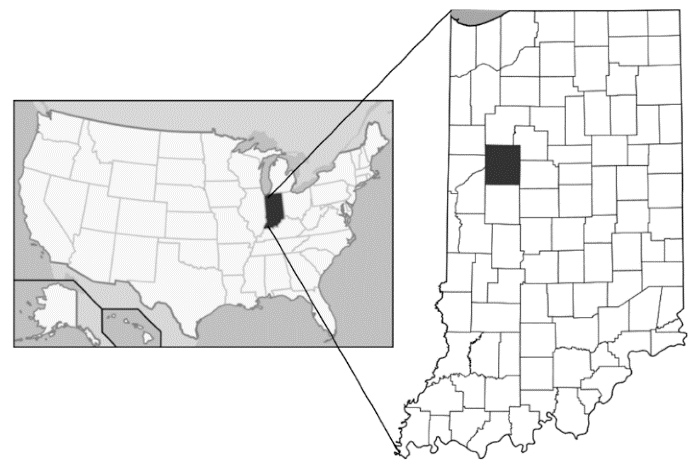
2. Data and Study Area

Tippecanoe County is located in north-central Indiana (Figure 2), including 10 cities/towns [36], with the total area of 503 square miles (approximate 1300 km2) [37]. The county-wide digital orthophoto mosaic of the National Agriculture Imagery Program (NAIP) consists of 47 Digital Orthophoto Quarter Quads (DOQQ). The 2010 NAIP data for Indiana were acquired between 18 June 2010 and 27 August 2010. These images contain four bands, including red (465–676 nm), green (604–664 nm), blue (533–587 nm), and near infra-red or NIR (420–492 nm). The spatial resolution of the orthophotography is 1 meter, and radiometric resolution is 8 bit, whose digital number (DN) values range from 0 to 255. The 2010 NAIP data are available in Tagged Image File Format (TIFF).
The digital elevation models (DEM) and digital surface models (DSM) were created from the Indiana Map Color Orthophotography Project in 2005, and both of them were generated by the State of Indiana’s vendor, Earth Data (ISDP 2005). The DEM and DSM data were collected during leaf-off conditions in March and April, with 5-foot (1.5 m) spatial resolution. The normalized digital surface model (NDSM) we utilized in our study is generated by subtracting the corresponding pixel values in the DEM from the DSM [38].
Figure 2. The study area is the Tippecanoe County that locates in the northwest quadrant of the U.S. state of Indiana.
Remotesensing 06 11372 g002

3. Methods

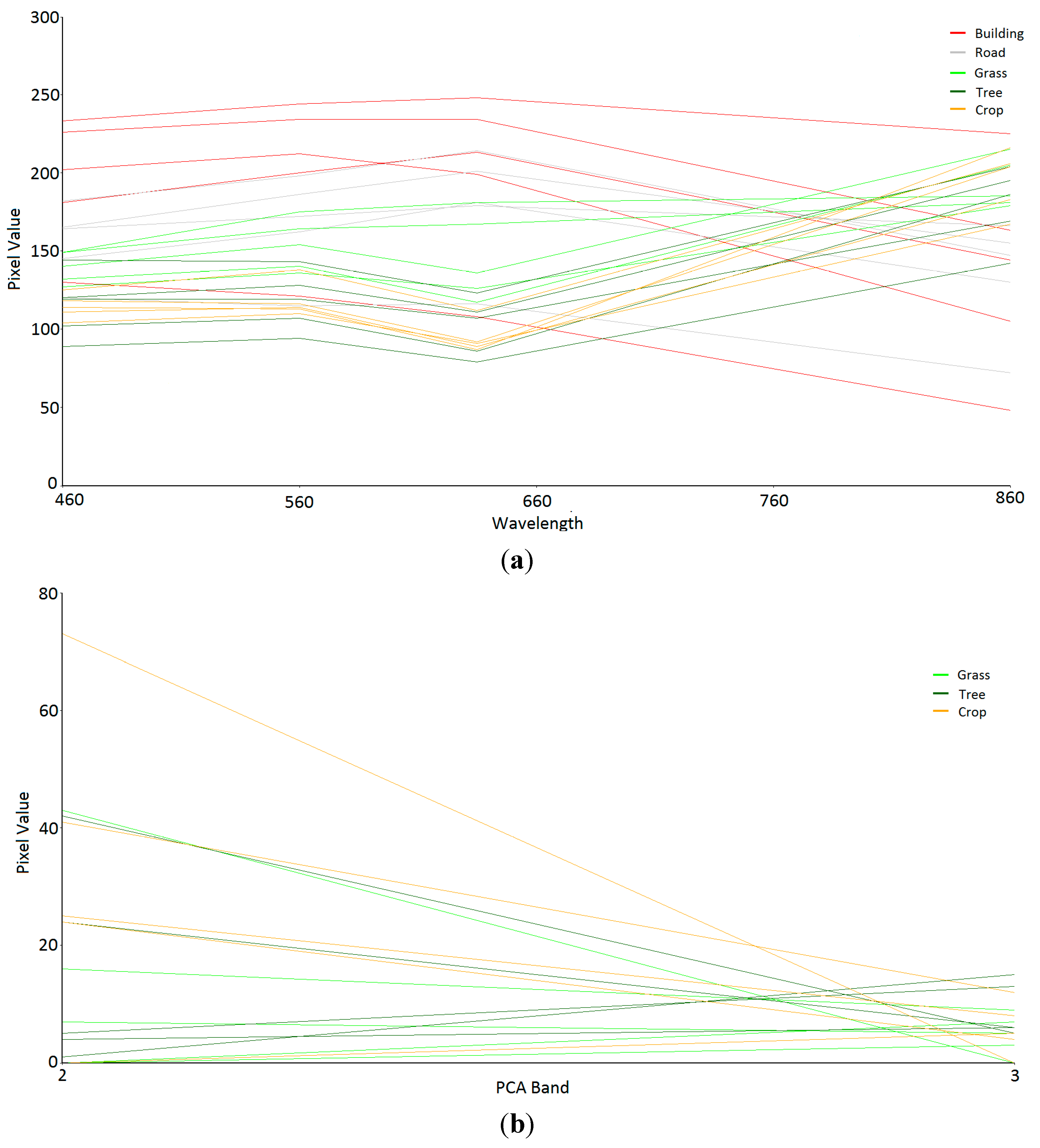
3.1. Spectral Information of Land-Cover Maps and Image Pre-Processing

Our methods attempt to distinguish land-cover types between buildings, roads (including parking lots and other impervious surfaces), open water (such as rivers, ponds and swimming pools), grass, tree (including urban tree and forest), open land/bare soil, and active cropland (cultivated vegetation covers for the active agricultural use). Figure 3 shows a series of spectral profiles that were derived from target pixels in our study area, where a variety of land cover types display intricate spectral characteristics both within and among classes. Therefore, using spectral information alone for land cover discrimination is not practical. Furthermore, similar to water bodies, shadows from tree canopies or high-rise buildings display low spectral reflectance. Pixel-based classification methods alone would misclassify large amounts of pixels and produce salt and pepper effects in the thematic map. To solve these two major issues, we pre-processed the original aerial photography using spectral transformations to enhance useful information while reducing the image spectral dimensions, and then employed OBIA for the image classification process.
After reprojecting all datasets to the coordinate system of Universal Transverse Mercator (UTM) Zone 16 North, North American Datum 1983 (NAD83), we utilized a principal component analysis (PCA) function to derive three new bands, which helped to reduce the spectral dimensions of the multivariate aerial photography and provided three uncorrelated variables to represent useful information (e.g., vegetation covers and imperious surfaces) contained in the RBG bands. The first PCA band captured the maximum amount of variation (81%) in the original bands of the aerial photograph. The second PCA band that explains 18% of the variance presented high brightness values in all vegetation covers, while maintaining variation in brightness values among the different vegetation types. The third PCA band (exhibits 1% of the variance) displayed extremely high and low brightness values in several specific vegetation types. We also used the Normalized Difference Vegetation Index (NDVI) to distinguish vegetation from non-vegetation pixels. We initially assigned pixels to vegetation class if their NDVI values were above zero; we recoded these as value “1” and all others as value “0”.
We used the binary NDVI image as a mask to split a PCA image into non-vegetation and vegetation parts which helps to reduce the space and time complexity in the object-based classification process. Each DOQQ area contains about 6000 × 7500 pixels with 4 bands, which results in more than 200 megabytes of data for each image. The space complexity does not allow a computer with less than 16G RAM memory to create more than three layers of segmentation levels for images at such size, and the computational time for images at such size highly depends on what feature extraction algorithms are used. Therefore, we separated the non-vegetation and vegetation parts in the image in order to reduce the computational time and fit the RAM limitation. Besides, we selected as few input image layers as possible, and kept as much useful information as possible for the object-based classification. For the vegetation part sub image, we chose PCA2 and PCA3 bands as input layers, because both bands include distinct vegetation information and exhibit differently in several vegetation types. For the non-vegetation part sub image, we selected PCA1, DOQQ band 4 (DOQ4), and NDSM band as input layers. This is because the PCA1 band consists of most of the information from aerial photography, and DOQ4 is an NIR band response which contains lower brightness values on impervious surfaces such as roads and parking lots. In addition, the NDSM band can assist in elevated objects delineation.
Figure 3. The image spectral response profiles showed that mixtures of spectral characteristics exited in the class of buildings and roads, and between different vegetation types in the original aerial photography bands and principal component analysis (PCA) bands. Lines in the figures with different colors represent different land-cover types. (a) The mixture in the spectral response of building and road objects, and the mixture in the spectral response of trees, crop and grass objects of 4-band aerial photos. (b) The mixture in the spectral response of trees, crop and grass objects of PCA bands.
Remotesensing 06 11372 g003

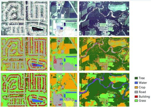
3.2. Object-Based Image Analysis

3.2.1. Image Segmentation

The segmentation process decomposes an image domain into a number of disjoint regions (image objects) so that the characteristics of the image objects within each region have high homogeneity and strong statistical correlations [14,39]. The segmentation algorithm first identifies a set of starting points (seed points) of a segmentation process and then joins contiguous pixels to the seed points if they fulfill the homogeneity criteria until certain thresholds are reached [40]. “Scale” is one of the important criteria in segmentation process. When the size of a growing region exceeds the threshold defined by the scale parameter, the merging process stops. Three criteria are defined in the Definiens software (formerly known as eCognition software) to constrain the pixel growing algorithm, namely color, shape and scale, to control smoothness and compactness of image objects [41]. Smoothness is defined as the ratio of an object’s perimeter to the perimeter of this object’s boundaries that run parallel to the image borders [42]; compactness is the ratio of an object’s perimeter to the square root of the number of pixels within that image object [40].
We used two segmentation algorithms in our study: multi-threshold (MT) segmentation and quadtree-based (QT). Although the commonly used multi-resolution (MR) segmentation is effective in separating an image into meaningful image objects, its processing time is much longer than that of QT and MT segmentation (approximate 10 time longer in our study), especially when it is applied to process large datasets. The segmentation algorithms used in this study tend to balance the computation time and product accuracy for the data-rich analyses in the complex landscape. MT segmentation splits an image object domain according to the pixel value(s) assigned to the thresholds [41]. QT segmentation represents images at multiple resolutions based on the pixel values within a given image object: the absolute difference of pixel values within the image object is compared with a threshold value (a user defined scale parameter). If the absolute difference is greater than the threshold, the segmentation process will decompose the image object into four new equally sized squares [43].
For images with vegetation portion, we executed the MT segmentation first to: (1) distinguish between the pure vegetation objects and mixed image objects; and (2) assign zero values to non-vegetation at a super level (coarser level). Secondly, we applied a second MT segmentation to extract grass, tree (mainly forest), and shadow objects from the vegetation image objects. Forest objects display the highest values in the PCA3 band, followed by grass, and shadows, thus we were able to distinguish these three classes by the brightness value of the PCA3 band. After that we utilized QT segmentation to split the images into a finer level of image object domains, with different scale parameters (Table 1), for both vegetation portions and non-vegetation portions respectively. As a result, large and square image objects were generated for areas with low spectral variation within large vegetation fields (e.g., regular rectangular crops and grass fields), whereas high spectral variation within heterogeneous areas, such as complicated urban centers, were segmented into small, square image objects. Because of higher spectral variances among the tree canopies, their image objects turned out to be much smaller than the size of crop objects after QT segmentation processes (Figure 4). Therefore spectral and spatial characteristics can be further used along with the geometry information to separate trees from other vegetation categories. For the non-vegetation part of the image segmentation processes, we employed MT segmentation at the very beginning to extract the water class which displays extremely low value in the DOQ4 band. A sub image object level was firstly created by QT segmentation, and the second sub image object level was generated by MT segmentation to delineate image objects that have above-zero heights by using the NDSM band.
Table 1. Segmentation methods and parameter settings used in the object-based classification procedures.
Parameters
Segmentation MethodsDomainScaleBand WeightThreshold
Vegetation Part
Band Included:
PCA2; PCA3
MT1All pixels50PCA2: 1non-vegetation ≤ 0
QT1All pixels100PCA2: 1--
MT2Unclassified25PCA3: 10 < grass ≤ 18
QT2Unclassified25PCA2: 0.5
PCA3: 0.5
--
Non-vegetation Part
Band Included:
PCA1; DOQ4; NDSM
MT1All pixels50DOQ4: 1vegetation ≤ 0
15 < water ≤ 80
QTAll pixels250PCA1: 0.5
DOQ4: 0.5
--
MT2All pixels100NDSM: 1non-elevated ≤ 0
Figure 4. The quadtree-based (QT) segmentation partitions an image into objects of trees (small squares) and crops (large squares). (a) Image of PCA2 band within a 800 × 1000 pixels area. (b) After the QT segmentation, most of the large squres represent the crops, and most of the small squares represent the trees. The blue squares are the non-vegetation image objects with assigned classes, whose borders were inherated from the upper level of Multi-threshold (MT) segmentation results.
Remotesensing 06 11372 g004

3.2.2. Vegetation Classification

We separated vegetation areas into three categories for each aerial photo: tree, grass, and crop. After a close examination of the characteristics of these three vegetation classes, we decided to delineate these vegetation objects using their own distinct spatial and spectral features so that we can find the boundaries of each vegetation type.
In the PCA2 band, a number of crop field objects exhibit extremely high brightness values, while other crop field objects display brightness values that are similar to those of trees and grass. In the PCA3 band, most tree objects show higher brightness values compared to crops and grass. Therefore, we initially delineated the “bright crops” by using brightness values from the PCA2 band (Mean_PCA2 > 140). For the remaining unclassified area (trees, grass and “dark crops”), spectral and geometry features were used together to delineate objects using a QT segmentation. A QT segmentation on the PCA3 band resulted in very small squares for most of the tree objects and larger squares for the areas with lower spectral variation, such as crop fields. Our selection criteria (Mean_PCA3 ≥ 25 AND Area < 1024 pixels) via observing the samples extracted most of trees from the unclassified image objects. Neighbors of tree objects were then merged to the tree class if they satisfied certain criteria, including area, relative border to the tree objects, and mean difference to the tree objects.
The grass class was initially separated using an MT segmentation based on brightness values in the PCA3 band. Grass objects were merged with neighboring objects that satisfied specified criteria in the aspects of size, mean difference, density, and relative border to the grass objects. The merging criteria for neighbor objects (relative border to grass class > 0) are area ≥ 4096 pixels and density ≥ 2.
D e n s i t y   =   # P v 1   +   V a r X   +   V a r Y
where Pv is the number of pixels; V a r X   +   V a r Y is the radius of the fitted ellipsoid [41].
Density, as formulated in Equation (1), describes the distribution of pixels within an image object [41]. Based on this formulation, a perfectly square object has the greatest possible density. As a result, the image object merging step grouped most square-shaped grass image objects. With most of the large areas of tree and grass identified, the remaining large unclassified image objects were patches of “dark crop”. We defined image objects with area ≥ 100,000 pixels as “dark crop”. For the tree classification rules, the unclassified objects with mean_PCA3 < 25 were classified as “dark crop”. We applied the QT segmentation for the second time with a smaller scale parameter to split the remaining unclassified image objects. This process helped to extract the remaining unclassified tree objects at a finer scale. Again, these image objects (with Mean_PCA3 ≥ 25 AND Area < 526 pixels) were assigned to the tree class.

3.2.3. Non-Vegetation Classification

Four categories were discriminated from the non-vegetation parts of the images: building, road (including parking lots and other non-elevated impervious surfaces), water, and open land (soil near water) (Figure 5). The most straightforward approach to extract buildings is to identify the elevated image objects with relatively regular shapes and certain criteria on the sizes in the segmented NDSM layer. We applied the MT segmentation process to the NDSM layer, and assigned elevated objects, e.g., elevation > 0 meter, to the building class. However, some elevated objects, such as elevated roads (overpass), were also extracted and wrongly assigned to the building class. In addition, the NDSM layer is not completely consistent with the aerial photography. The elevation model data were collected earlier (in 2005) than the aerial photos (in 2010). As a result, some buildings shown in the NDSM data had been removed at that time of 2010, and are not shown on the aerial photographs. Newly constructed buildings after 2005 appear on aerial photographs but not in the NDSM data. In either case, the MT segmentation process cannot completely separate all buildings from other impervious surfaces, such as roads and parking lots. Moreover, spectral overlapping between roof and a number of other image objects (e.g., parking lots) prevented the complete separation of buildings. Therefore we have to rely on expert knowledge regarding spatial, textural, and geometric characteristics of image objects.
Figure 5. A binary diagram of the object-based rule used in the classification.
Remotesensing 06 11372 g005
After classifying the vegetation objects, we distinguished the non-vegetated objects. First, we identified road and building categories according to their elevation, area, shape and brightness values in the PCA1 band. The remaining unclassified image objects were classified based on their spatial relationships. Finally, misclassified objects, such as road, building and water, were examined and reclassified using their geometry and spatial relationship features.
The first step in the non-vegetation classification was to extract road image objects. Expert knowledge in spatial and spectral features was applied to identify roads. We used the “multi-resolution segmentation region grow” (MRSRG) algorithm in three continuous steps to reshape and merge segmented image objects based on the MR segmentation criteria [40] (Figure 6). As to the parameter settings, the PCA1 band was selected as the only active layer for image object growth. The respective homogeneity criteria for each segmentation were: (1) scale = 10,000, shape = 0.1, compactness = 0.5; (2) scale = 250, shape = 0.3, compactness = 0.5; and (3) scale = 50, shape = 0.5, compactness = 0.8. These three segmentations first targeted large areas with an emphasis on spectral information, then smaller areas with an emphasis on object shapes. The last segmentation step merged the objects with similar mean brightness values. The results of both MR segmentation) and spectral difference (SD) segmentation (growing image objects based on their brightness values with specific criteria) were similar. The expert rules for road extraction include mean layer values, geometry, and class-related features, demonstrated in Table 2.
Table 2. Classification Specification for Road Classes.
Road Class 1Road Class 2Road Class 3Road Class 4
Mean PCA1 ≥ 320Mean PCA1 ≥ 350Density Mean ≤ 1.5Mean NDSM ≤ 5
Rel. border to road3 ≥ 0.25
Mean Absolute difference of Mean PCA1 compare to road1 ≤ 50
Density ≤ 1.5Mean NDSM ≤ 5Mean PCA1 ≥ 100
Mean NDSM ≤ 5 Rel. border to road1 > 0
100 ≤ Area ≤ 10,000 pixels Shape index ≤ 2
Road Class 5Road Class 6
Area ≤ 2000 pixelsMean NDSM ≤ 5
Mean PCA1 ≥ 300Rel. border to road5 ≥ 0.4
Figure 6. The building and road image objects were effectively refined and merged after using multi-resolution image region grow algorithm (MRSRG). (a) The building and road image objects after quadtree-based segmentation. (b) Image objects after the first time of MRSRG with parameters: scale = 10,000, shape = 0.1, compactness = 0.5. (c) Image objects after the second time of MRSRG with parameters: scale = 250, shape = 0.3, compactness = 0.5. (d) Image objects after the third time of MRSRG with parameters: scale = 50, shape = 0.3, compactness = 0.8.
Remotesensing 06 11372 g006
Building objects are either adjacent to or mixed with the road objects, and elevation and spectral information cannot completely separate buildings from road objects. Therefore, we first distinguished building objects based on their NDSM information at the pixel level. The image objects with height above zero are assigned to the “elevated” class. Those elevated objects were then merged into building objects if they satisfy the criteria listed in Table 3. The feature shape index (shown in the Equation (2)) that described the smoothness of an image object’s border was used in extracting compact and smooth road segments from building objects. Shape index is calculated from the image object’s border length divided by four times the square root of its area [41].
S h a p e   i n d e x   =   b v 4 # P v
where bv is the image object’s border length; 4 # P v is the border of a square area with Pv number of pixels [41].
Table 3. Classification specification for building classes.
Building Class 1Building Class 2Building Class 3Building Class 4
NDSM > 0 (elevated)NDSM > 10Rel. Border to Building1 > 0Mean PCA1 > 300
Mean Absolute difference of Mean NDSM compare to elevated ≤ 50Rel. Border to Building1 ≥ 0.5Mean Absolute difference of Mean PCA1 compare to Buildings 1 and 2 ≤ 20Density ≥ 1.8
Density > 1
Area ≥ 64 pixels
After applying the above rules, most buildings, roads, water and open land were assigned to the corresponding categories. However, a number of road image objects were misclassified as buildings either because their mean layer brightness values were similar, or the road objects contained high elevation features (e.g., a few patches of overpass and filament road objects have been classified as buildings). In addition, multiple road objects (asphalt parking lots) with low reflectance were mislabeled and assigned to the water class. Therefore, we also defined and applied separation rules for both buildings and water image objects (shown in Table 4). After applying these rules, the misclassified objects were reclassified to road. Other remaining small unclassified image objects were merged to different classes based on the weight of their relative borders to each category.
Table 4. Rules for reclassification of mislabeled building image objects and water image objects.
To Road Class 1To Road Class 2To Road Class 3To Road Class 4To Road Class 5
Building ClassDensity < 1.2Rel. border to Road > 0.75
Area ≤ 100 pixelsMean NDSM < 8
Water ClassMean NDSM > 0Area ≤ 500 pixelsArea ≤ 1000 pixelsArea ≤ 2000 pixelsArea ≤ 5000 pixels
Mean PCA1 ≥ 200Rel. border to Road ≥ 0.5 Rel. border to Road > 0.75Rel. border to Road > 0.25
Shape index > 2.5

4. Results and Discussion

Our OBIA approach generated a land-cover map of Tippecanoe County in the state of Indiana with 7 classes. The county examined is composed of 2.64% (34.7 km2) buildings of all kinds; 5.08% (66.9 km2) non-building asphalt and concrete; 3.45% (45.4 km2) bare soil/rock; 28.04% (369.4 km2) vegetation (14.91% tree/forest and 13.13% grass,); 59.66% (785.7 km2) active cultivated cropland; and 1.13% (14.9 km2) open water bodies. The classification results of our object-based approach were compared against that of traditional pixel-based method with supervised classification. The four-band aerial photographs were used as input data for the pixel based method, and the training samples for every class were selected by using the experts’ prior knowledge, and the polygons of pixels were digitized for those categories. The sample size for the single family residential building is approximate 50 pixels, and the sample sizes for other categories are least 100 pixels. We used the stratified random sampling accuracy assessment with approximate 80 random selected points per class (600 points total) to validate the classification results (in ERDAS software). The overall accuracy of our OBIA classification results achieved 93% (Table 5), compared to the maximum likelihood pixel based method (over all accuracy = 79%) that we tested in our research (Table 6).
Table 5. Accuracy assessment on classification result using Object-Based Imagery Analysis (OBIA).
Kappa %Reference Total CountMap Total CountNumber of CorrectProducer’s Accuracy (PA) %User’s Accuracy (UA) %
Building84.51627262100.0086.11
Road95.4078757292.3196.00
Tree/Forest91.8189868089.8993.02
Grass87.7177847597.4089.29
cropland96.1115914013685.5397.14
Water88.83637063100.0090.00
Openland/
Bare soil
96.8972737198.6197.26
Overall accuracy = 93.17%; Overall Kappa statistics = 91.9%
Table 6. Accuracy assessment on classification result using pixel-based method.
Kappa %Reference Total CountMap Total CountNumber of CorrectProducer’s Accuracy (PA) %User’s Accuracy (UA) %
Building60.3367825379.1064.63
Road76.5092806469.5780.00
Tree/Forest76.31961108891.6780.00
Grass75.9798947576.5379.79
Cropland82.49108907771.3085.56
Water87.0780807188.7588.75
Openland/
Bare soil
73.2576816281.5876.54
Overall accuracy = 79.42%; Overall Kappa statistics = 75.95%
The OBIA method provided a robust classification result for the fine resolution land-cover mapping, and it can be used to facilitate a large amount of researches and managements in terms of the landscape planning, regional land-use and land-cover changes, environmental and sustainability as noted in the beginning of this paper. By using OBIA classification method for the land-cover mapping in our study, we identified three representative areas to demonstrate the benefit of using object-based methods (Figure 7, tables 5 and 6). In the pixel-based classification results, “salt and pepper” effects were apparent. Also, the crop class was frequently confused with the grass and tree classes using pixel-based approaches; buildings are easily misclassified as soil, road, and parking lot. As a result, a number of grass areas were incorrectly classified as crops and were frequently located in urban, residential areas, and forest areas. The spectral similarities within the different land-cover types (especially for those similar materials) cannot be effectively separated them without other characteristics from the ground objects. On the other hand, the object-based approach was able to separate crops and grass objects, as well as to distinguish shadows from grass. Moreover, the elevation model cannot be used directly in the pixel-based method, thus a number of buildings, which had similar spectral responses to roads, were classified as road and vice versa. In addition, rivers have low spectral reflectance, which is similar to some asphalt roofs and road segments, so they were frequently classified as buildings or roads classes. The object-based method integrated NDSM data that can extract, group, and reshape elevated objects and separated image objects with comparable brightness value.
Figure 7. A comparison between pixel-based and object-based classification results. The first row shows the image of original DOQQ with RGB band combination display. The second row of images is the pixel-based classification results. The third row of image is the object-based classification results. Each column shows the same location on the map.
Remotesensing 06 11372 g007
Our study area is covered by 47 aerial photo quarter quads with corresponding NDSM datasets, totaling 26 Gigabyte of data. In order to reduce the time and memory demands of the class delineation process, we conducted a PCA and NDVI transformation on the original four-band data, thus creating more compact inputs with useful information. Different band combinations were selected as the input layers for object-based image classification of the vegetation and non-vegetation portions of the images. In addition, we utilized segmentation algorithms with less computationally demanding (QT and MT segmentation methods) to divide image domains into objects and only included features that contributed to the object separation.
QT segmentations at multiple scales were used to extract the tree objects. Using multiple scales provides two benefits. First, after applying several scale parameters in the QT segmentation, we found that 100 was the best value for the initial segmentation, as it generated moderate sized objects with distinctive features. When using scale parameter higher than 100, the QT segmentation did not generate adequate objects; when using scale parameter lower than 100, much more information was generated and the program terminated due to the overflow of random-access memory (RAM). Second, when an image domain contains a specific class of object (e.g., tree canopy objects), we employed QT segmentation again with smaller scale parameters to obtain small object squares if their neighbors have apparent variance in pixel values. The repeated QT segmentation at finer scales is similar to using some types of texture analysis, but with reduced computation cost. One drawback of our method is that it produces zigzag edges in many patches of vegetation. This is mainly because of the restricted shape (square) of image objects generated in the QT segmentation process.
We classified vegetation types in an order that mimic the human recognition and mitigate the redundancy within the feature extraction processes: first bright colored crops, then trees, followed by dark colored crops, and finally grass. In theory, each vegetation type can be discriminated regardless of the classification order. However, using a systematic order can enhance the efficiency of the object delineation process. For example, the PCA2 band response showed very high brightness values in certain crop fields, which we named as “bright crops”. Meanwhile in the PCA3 band, those same “bright crops” displayed brightness values similar to the tree class. Therefore, first extracting the “bright crops” via mean PCA2 band brightness values helped to reduce confusion in tree class discrimination. Most tree areas, especially forest areas, were divided into small square objects due to the high spectral variation in the tree canopy pixel values and shadows in the tree canopies. We first utilized mean layer values to discriminate tree objects, as grass and shadow objects have low mean layer values in the PCA2 and PCA3 bands. Then we examined neighbors of tree objects to identify shadow objects. According to their geometry (area) and spatial relationship (relative border to tree) features, shadow and tree objects were identified respectively. Finally, the remaining unclassified objects with low mean layer value objects were assigned to the grass class.
During the feature selection and extraction procedures, we used the “multi-resolution segmentation region grow” (MRSRG) process to merge image objects. This process is similar to the spectral difference (SD) segmentation process that grows neighboring image objects according to their mean image layer intensity values and merges neighboring objects based on user-defined spectral difference criteria [40]. Although SD segmentation is designed to reshape existing image objects, when it deals with large image datasets such as a subset of our study area, the computational time is much greater than that of the MRSRG method. After the QT segmentation, we also used density and shape index features to separate buildings and roads. These features yielded more effective and efficient results than the “ratio of length to width” feature.
The NDSM datasets were generated from the 2005 Indiana Map Digital Elevation and Surface Models. Due to a discrepancy in the time of measurement, the 2010 NAIP data are not completely comparable with the NDSM data. Identification of missing and recently constructed building objects requires additional datasets. Furthermore, the inaccuracy of elevation data in the NDSM dataset introduced error when comparing the heights among objects. A few water objects, such as ponds, displayed a positive value, while a number of the elevated objects and roads have negative value on the NDSM layer. Inaccurate elevation information resulted in the misclassification of a few image objects. We did not use NDSM datasets for tree delineation because the NDSM datasets have a spatial resolution of 5 feet, which was not fine enough to capture the elevation of trees in our study area.

5. Conclusions

The object-based approach was used to classify high-resolution aerial photography and ancillary elevation data for relatively more detailed land cover mapping. The classification results show that this approach is more effective than pixel-based methods in terms of classification accuracy. While only spectral reflectance is considered in pixel-based approaches, the OBIA method utilizes multiple segmentation algorithms that help improve classification accuracy. Using elevation and spatial relationship information, image objects with similar spectral responses can be effectively differentiated and assigned to corresponding classes. This study also demonstrates an efficient method for land-cover mapping with very high spatial resolution images at a relatively broader spatial scale. Spectral transformation and separation of the land type within the imagery can be performed to reduce complexity and work load during the OBIA process. These are essential procedures to maintain reasonable computational cost while processing large-area high-resolution images. Parameters used in the rule sets are sample values specifically for the study area we chose, and may vary for other locations of interest, but the similar principles and procedures can be applied to other areas. Using additional ancillary data, such as 1-meter resolution LiDAR (Light Detection and Ranging) may further help generate more accurate land-cover maps, which is among our planned future work.

Acknowledgments

The authors would like to acknowledge the department of Forestry and Natural Resources at Purdue University for support in this study.

Author Contributions

Xiaoxiao Li and Guofan Shao conceived the research; Xiaoxiao Li carried out the research; Xiaoxiao Li and Guofan Shao wrote the paper.

Conflicts of Interest

The authors declare no conflict of interest.

References

  1. Ben Dor, E. Imagery spectrometry for urban applications. In Imaging Spectrometry; van der Meer, F.D., de Jong, S.M., Eds.; Springer: Dordrecht, The Netherlands, 2006; pp. 243–281. [Google Scholar]
  2. Tooke, T.R.; Coops, N.C.; Goodwin, N.R.; Voogt, J.A. Extracting urban vegetation characteristics using spectral mixture analysis and decision tree classifications. Remote Sens. Environ. 2009, 113, 398–407. [Google Scholar]
  3. Li, X.; Myint, S.W.; Zhang, Y.; Galletti, C.; Zhang, X.; Turner, B.L., II. Object-based land-cover classification for metropolitan Phoenix, Arizona, using aerial photography. Int. J. Appl. Earth Obs. Geoinf. 2014, 33, 321–330. [Google Scholar] [CrossRef]
  4. Turner, B.L.; Janetos, A.C.; Verburg, P.H.; Murray, A.T. Land system architecture: Using land systems to adapt and mitigate global environmental change. Glob. Environ. Change 2013, 23, 395–397. [Google Scholar] [CrossRef]
  5. Wu, J.G. Landscape sustainability science: Ecosystem services and human well-being in changing landscapes. Landsc. Ecol. 2013, 28, 999–1023. [Google Scholar] [CrossRef]
  6. Myint, S.W.; Gober, P.; Brazel, A.; Grossman-Clark, S.; Weng, Q. Per-pixel vs. object-based classification of urban land cover extraction using high spatial resolution imagery. Remote Sens. Environ. 2011, 115, 1145–1161. [Google Scholar]
  7. Peña-Barragán, J.M.; Ngugi, M.K.; Plant, R.E.; Six, J. Object-based crop identification using multiple vegetation indices, textural features and crop phenology. Remote Sens. Environ. 2011, 115, 1301–1316. [Google Scholar] [CrossRef]
  8. Ellis, E.C.; Wang, H.Q.; Xiao, H.S.; Peng, K.; Liu, X.P.; Li, S.C.; Ouyang, H.; Cheng, X.; Yang, L.Z. Measuring long-term ecological changes in densely populated landscapes using current and historical high resolution imagery. Remote Sens. Environ. 2006, 100, 457–473. [Google Scholar] [CrossRef]
  9. Zhou, W.; Troy, A.; Grove, M. Object-based land cover classification and change analysis in the Baltimore metropolitan area using multitemporal high resolution remote sensing data. Sensors 2008, 8, 1613–1636. [Google Scholar] [CrossRef]
  10. Chen, Y.; Shi, P.; Fung, T.; Wang, J.; Li, X. Object-oriented classification for urban land cover mapping with ASTER imagery. Int. J. Remote Sens. 2007, 28, 4645–4651. [Google Scholar] [CrossRef]
  11. Nichol, J.; King, B.; Quattrochi, D.; Dowman, I.; Ehlers, M; Ding, X. Earth observation for urban planning and management: State of the art and recommendations for application of earth observation in urban planning. Photogramm. Eng. Remote Sens. 2007, 73, 973–979. [Google Scholar]
  12. Nichol, J.; Lee, C.M. Urban vegetation monitoring in Hong Kong using high resolution multispectral images. Int. J. Remote Sens. 2005, 26, 903–918. [Google Scholar] [CrossRef]
  13. Cadenasso, M.L.; Pickett, S.T.A.; Schwarz, K. Spatial heterogeneity in urban ecosystems: Reconceptualizing land cover and a framework for classification. Front. Ecol. Environ. 2007, 5, 80–88. [Google Scholar] [CrossRef]
  14. Blaschke, T.; Hay, G.J.; Weng, Q.; Resch, B. Collective sensing: Integrating geospatial technologies to understand urban systems—An overview. Remote Sens. 2011, 3, 1743–1776. [Google Scholar] [CrossRef]
  15. Stow, D.; Coulter, L.; Kaiser, J.; Hope, A.; Service, D.; Schutte, K. Irrigated vegetation assessment for urban environments. Photogramm. Eng. Remote Sens. 2003, 69, 381–390. [Google Scholar] [CrossRef]
  16. Guisan, A.; Thuiller, W. Predicting species distribution: Offering more than simple habitat models. Ecol. Lett. 2005, 8, 993–1009. [Google Scholar] [CrossRef]
  17. Mehrabian, A.; Naqinezhad, A.; Mahiny, A.S.; Mostafavi, H.; Liaghati, H.; Kouchekzadeh, M. Vegetation mapping of the Mond Protected Area of Bushehr Province (south-west Iran). J. Integr. Plant Biol. 2009, 51, 251–260. [Google Scholar] [CrossRef] [PubMed]
  18. Hester, D.B.; Cakir, H.I.; Nelson, S.A.C.; Khorram, S. Per-pixel classification of high spatial resolution satellite imagery for urban land-cover mapping. Photogramm. Eng. Remote Sens. 2008, 74, 463–471. [Google Scholar] [CrossRef]
  19. Park, M.H.; Stenstrom, M.K. Classifying environmentally significant urban land uses with satellite imagery. J. Environ. Manag. 2008, 86, 181–192. [Google Scholar] [CrossRef]
  20. Myint, S.W.; Mesev, V.; Lam, N. Urban textural analysis from remote sensor data: Lacunarity measurements based on the differential box counting method. Geogr. Anal. 2006, 38, 371–390. [Google Scholar] [CrossRef]
  21. Weng, Q.; Lu, D. A sub-pixel analysis of urbanization effect on land surface temperature and its interplay with impervious surface and vegetation coverage in Indianapolis, United States. Int. J. Appl. Earth Obs. Geoinf. 2008, 10, 68–83. [Google Scholar] [CrossRef]
  22. Mallinis, G.; Koutsias, N.; Tsakiri-Strati, M.; Karteris, M. Object-based classification using Quickbird imagery for delineating forest vegetation polygons in a Mediterranean test site. ISPRS J. Photogramm. Remote Sens. 2008, 63, 237–250. [Google Scholar] [CrossRef]
  23. Zhou, W.; Huang, G.; Troy, A.; Cadenasso, M.L. Object-based land cover classification of shaded areas in high spatial resolution imagery of urban areas: A comparison study. Remote Sens. Environ. 2009, 113, 1769–1777. [Google Scholar] [CrossRef]
  24. Blaschke, T.; Hay, G.J.; Kelly, M.; Lang, S.; Hofmann, P.; Addink, E.; Feitosa, R.Q.; van der Meer, F.; van der Werff, H.; van Coillie, F.; et al. Geographic object-based image analysis—Towards a new paradigm. ISPRS J. Photogramm. Remote Sens. 2014, 87, 180–191. [Google Scholar] [CrossRef]
  25. Blaschke, T.; Lang, S.; Lorup, E.; Strobl, J.; Zeil, P. Object-oriented image processing in an integrated GIS/remote sensing environment and perspectives for environmental applications. In Environmental Information for Planning, Politics and the Public; Cremers, A., Greve, K., Eds.; Metropolis Verlag: Marburg, Germany, 2000; pp. 555–570. [Google Scholar]
  26. Blaschke, T. Object based image analysis for remote sensing. ISPRS J. Photogramm. Remote Sens. 2010, 65, 2–16. [Google Scholar] [CrossRef]
  27. Li, X.; Shao, G. Object-based urban vegetation mapping with high-resolution aerial photography as a single data source. Int. J. Remote Sens. 2012, 34, 771–789. [Google Scholar] [CrossRef]
  28. Baatz, M.; Schäpe, M. Multiresolution segmentation: An optimization approach for high quality multi-scale image segmentation. In Angewandte Geographische Informations-Verarbeitung XII; Strobl, J., Blaschke, T., Griesebner, G., Eds.; Wichmann Verlag: Karlsruhe, Germany, 2000; pp. 12–23. [Google Scholar]
  29. Blaschke, T.; Strobl, J. What’s wrong with pixels? Some recent developments interfacing remote sensing and GIS. GeoBIT/GIS 2001, 6, 12–17. [Google Scholar]
  30. Burnett, C.; Blaschke, T. A multi-scale segmentation/object relationship modelling methodology for landscape analysis. Ecol. Model. 2003, 168, 233–249. [Google Scholar] [CrossRef]
  31. Blaschke, T.; Burnett, C.; Pekkarinen, A. Image segmentation methods for object-based analysis and classification. In Remote Sensing Image Analysis: Including the Spatial Domain; Springer: Berlin, Germany, 2004; pp. 211–236. [Google Scholar]
  32. Hay, G.J.; Castilla, G.; Wulder, M.A.; Ruiz, J.R. An automated object-based approach for the multiscale image segmentation of forest scenes. Int. J. Appl. Earth Obs. Geoinf. 2005, 7, 339–359. [Google Scholar] [CrossRef]
  33. Xian, G.; Homer, C. Updating the 2001 National Land Cover Database impervious surface products to 2006 using Landsat imagery change detection methods. Remote Sens. Environ. 2010, 114, 1676–1686. [Google Scholar] [CrossRef]
  34. National Agricultural Statistics Database. 2010; National Agricultural Statistics Service-Official Site. Available online: http://www.nass.usda.gov/ (accessed on 3 May 2010). [Google Scholar]
  35. Liu, Z.; Wang, J.; Liu, W. Building extraction from high resolution imagery based on multi-scale object oriented classification and probabilistic Hough transform. In Proceedings of the IEEE International Geoscience and Remote Sensing Symposium, IGARSS ’05, Seoul, Korea, 25–29 July 2005; 2005; pp. 2250–2253. [Google Scholar]
  36. Indiana Spatial Data Portal. Indiana Geological Survey-Official Site. 2010. Available online: http:// igs.indiana.edu/ (accessed on 3 June 2010).
  37. Census Gazetteer Data for United States counties. 2010; United States Census Bureau. Available online: http://www.census.gov/tiger/tms/gazetteer/county2k.txt (accessed on 11 December 2010). [Google Scholar]
  38. Tovari, D.; Vogtle, T. Object classification in laser scanning data. In Proceedings of the ISPRS Working Group VIII/2, Laser-Scanners for Forest and Landscape Assessment, Freiburg, Germany, 3–6 October 2004; pp. 45–49.
  39. Benz, U.C.; Hofmann, P.; Willhauck, G.; Lingenfelder, I.; Heynen, M. Multi-resolution, object-oriented fuzzy analysis of remote sensing data for GIS-ready information. ISPRS J. Photogramm. Remote Sens. 2004, 58, 239–258. [Google Scholar] [CrossRef]
  40. Elmqvist, B.; Ardo, J.; Olsson, L. Land use studies in drylands: An evaluation of object-oriented classification of very high resolution panchromatic imagery. Int. J. Remote Sens. 2008, 29, 7129–7140. [Google Scholar] [CrossRef]
  41. Definiens. In Definiens eCognition Developer 8 Reference Book; Definiens AG: München, Germany, 2009.
  42. Feitosa, R.Q.; Costa, G.A.; Cazes, T.B.; Feijó, B. A genetic approach for the automatic adaptation of segmentation parameters. In Proceedings of the First International Conference on Object-Based Image Analysis, Salzburg, Austria, 4–5 July 2006.
  43. Chang, S.; Messerschmitt, D.G. Comparison of transform coding techniques for arbitrarily-shaped image segments. Multimed. Syst. 1994, 1, 231–239. [Google Scholar] [CrossRef]

