3.1. Modulated RSR
The NASA DNB radiometric calibration method uses a time-dependent RSR to model the optical change in the mirror property. The S-NPP VIIRS RTA throughput has degraded significantly during the course of on-orbit operations due to unexpected mirror darkening [
15]. Because the degradation is wavelength dependent, it has resulted in a significant change to the DNB RSR within its wide band pass. In DNB radiometric calibration, the RSR is used to determine the proportion of solar irradiance at each spectral wavelength received by the detectors [
8]. A change in RSR will affect the total radiance received by the detector. To accurately compute the DNB gains, a time-dependent modulated RSR is used to model the change of incident solar radiance expected during solar calibration events.
Based on the optical throughput degradation model [
16], we compute the time-dependent modulated DNB RSR at time
t as,
In Equation (1),
RSRmodulated is the modulated RSR,
RSRoriginal is the pre-launch measured RSR and
D is the degradation factor at wavelength
λ and time
t.
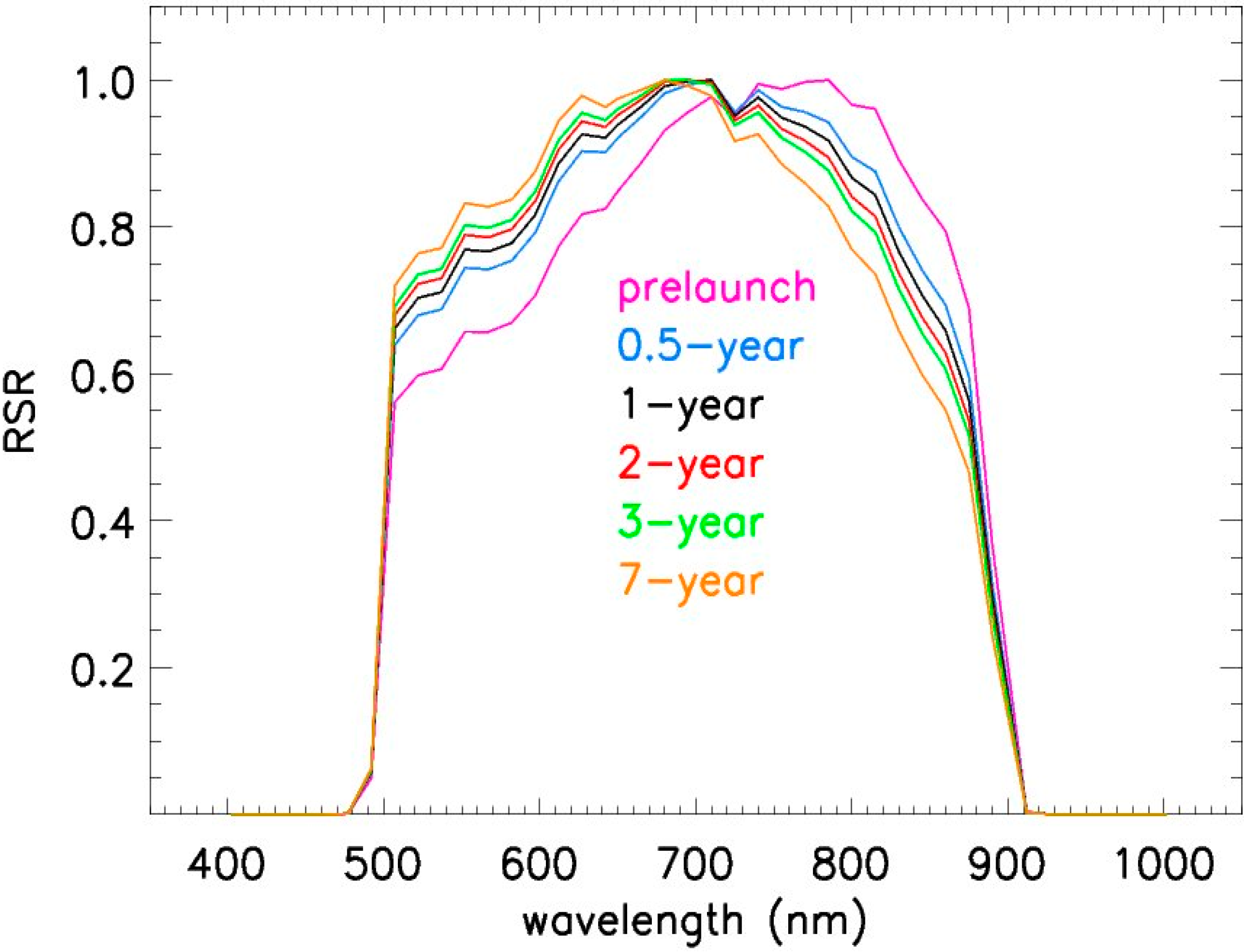
Figure 2 shows the pre-launch measured RSR and the computed modulated DNB RSRs at 0.5, 1, 2, 3 and 7 years post-launch based on degradation factors estimated from reflective solar band (RSB) calibration coefficient F-factors [
16]. The time series of modulated RSRs show that the relative response has shifted to lower wavelengths over time. The peak response has been lowered from ~790 nm to ~700 nm, and the RSR has increased/decreased for wavelengths under/over 700 nm. The rate of RSR modulation change was fastest in the early months of the S-NPP mission when the throughput degradation was most rapid.
Figure 2.
Modulated relative spectral responses (RSRs) computed based on current and projected rotating telescope assembly (RTA) mirror degradation trends at selected time intervals.
Figure 2.
Modulated relative spectral responses (RSRs) computed based on current and projected rotating telescope assembly (RTA) mirror degradation trends at selected time intervals.
The calibration biases associated with the DNB RSR modulation can be demonstrated by comparing the gains computed using pre-launch RSR and time-dependent RSRs.
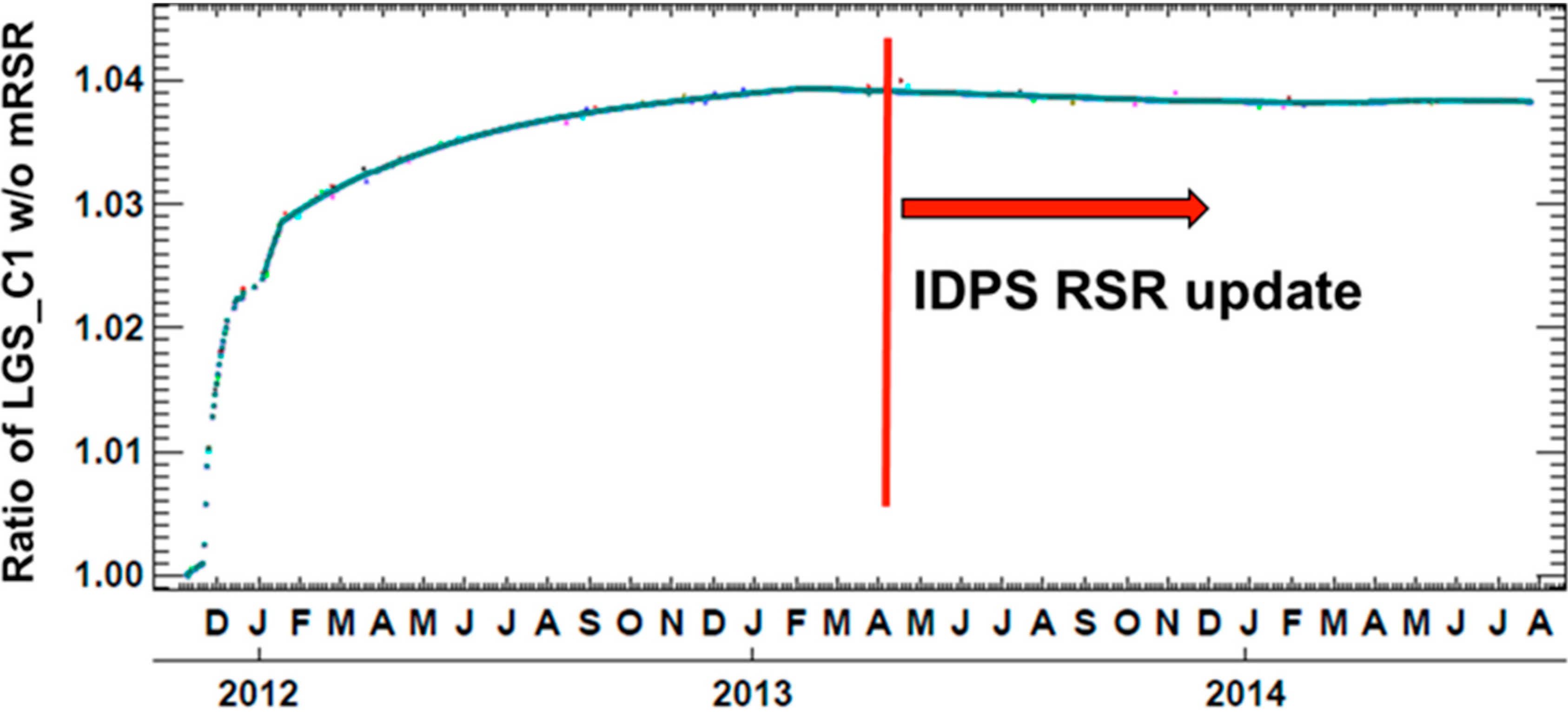
Figure 3 shows that the modulated RSR impact on LGS gain has been about 4% since the launch, and three quarters of the total change (~3%) occurred before the DNB CCD reached operational temperature (20 January 2012). The same modulated RSR impact is expected for the MGS and HGS, as they shared the same optical path as the LGS. To propagate the modulated RSR impact, the MGS and HGS gains are determined from the LGS gains computed with the time-dependent modulated RSR, as well as with the MGS/LGS and HGS/MGS gain ratios.
Figure 3.
The ratios of LGS gains computed with and without using the time-dependent modulated RSRs. The vertical line indicates the timing of the Interface and Data Processing Segment (IDPS) RSR update.
Figure 3.
The ratios of LGS gains computed with and without using the time-dependent modulated RSRs. The vertical line indicates the timing of the Interface and Data Processing Segment (IDPS) RSR update.
In April 2013, the JPSS SDR calibration team updated RSR LUTs with modulated RSRs, including DNB, in an offline calibration process to reflect the RSR impact on the calibration coefficients. The IDPS calibration process does not include the capability of time-dependent RSR correction, because the large RTA degradation in S-NPP VIIRS was not anticipated pre-launch [
15].
Figure 3 shows that the modulated RSR impact on DNB gain had diminished around the time of the IDPS RSR update. The timing of the RSR update has proven to be adequate for near-term purposes, as the rate of RSR modulation changes are diminishing based on the current projected RSR change (
Figure 2). To provide the best radiometric accuracy, the NASA VCST continues to compute DNB gain using the time-dependent RSR and to recommend DNB RSR updates when necessary.
3.2. EV Dark Offset Reference
The NASA DNB calibration methodology requires an EV dark offset reference point to determine the time-dependent EV dark offset from the BB dark offset drift [
8,
13]. The accuracy of the reference EV dark offset is vital, because the errors in the reference offset will be carried over to the entire time series. Currently, the S-NPP flight team performs a special VIIRS recommended operating procedure, VROP702, at the new moon each month to obtain EV dark offset by collecting data over the dark ocean [
17]. The dark ocean scene is sufficiently dark for the LGS and MGS, but not for the HGS, due to the effects of airglow. This airglow impact was not anticipated pre-launch partly due to the fact that its magnitude is lower than the DNB’s design dynamic range (3 × 10
−9 W∙cm
−2∙sr
−1). However, on-orbit analysis has shown that the usable DNB dynamic range is over the design minimum, especially for samples close to the scan nadir [
6] (also see
Section 4). An airglow-free EV dark reference is desired for this data collection, because of the superior sensitivity of the DNB detectors.
To establish an airglow-free HGS offset, the deep space scene collected during the S-NPP spacecraft pitch maneuver [
18] is used. An S-NPP pitch maneuver was performed during the new moon on 20 February 2012, which was one day before the VIIRS DNB offset determination procedure (VROP702) was performed. During the VROP702, the DNB sensor was commanded to report either HGA or HGB instead of the HGS (mean of HGA and HGB) that it reports during normal operation. During the pitch maneuver, the DNB sensor was configured in normal operational mode, and the HGS data were collected during the maneuver.
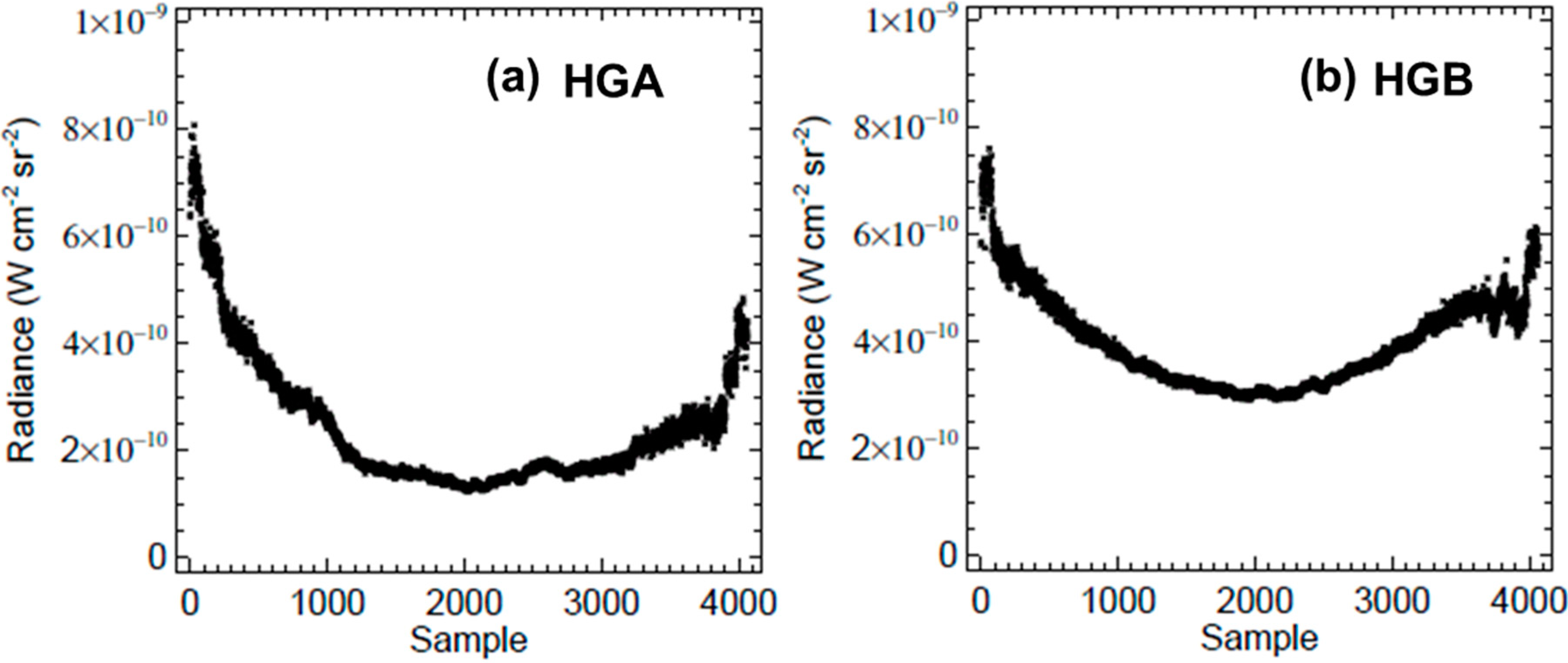
Figure 4 shows the difference of Earth scene radiance retrieval between VROP702 (looking down at the dark ocean) and pitch maneuver (looking up into deep space). It shows that the VROP702 scene radiance is generally higher than the pitch maneuver scene radiance. The biases are higher for the HGB than for the HGA, and both show a skewed symmetrical pattern with a magnitude from 2 to 8 ×10
−10 W∙cm
−2∙sr
−1. The airglow is stronger at higher scan angles where longer atmospheric path radiance is collected. The higher HGB-HGS biases are likely the result of stronger airglow within the VROP702’s HGB collection region than within the HGA collection region [
17].
Figure 4.
The radiance difference between the pitch maneuver deep space view (performed on 20 February 2012) and the VROP702 (VIIRS recommended operating procedure) dark ocean view (performed on 21 February 2012). (a) VROP702 HGA-pitch HGS; (b) VROP702 HGB-pitch HGS. Plots show detector averaged biases; the detector dependent airglow intensity could be higher or lower.
3.3. Gain and Offset Trending
The partnership between NASA VCST and Land PEATE provides users with mission-wide calibrated DNB data based on the latest calibration algorithm. Here, we show the mission-wide gain and offset used in the latest Land PEATE reprocessed DNB SDRs [
19] and compare them with the gain and offset used in the existing IDPS DNB data products. The comparisons for LGS, MGS and HGS are shown in
Figure 5,
Figure 6 and
Figure 7, respectively.
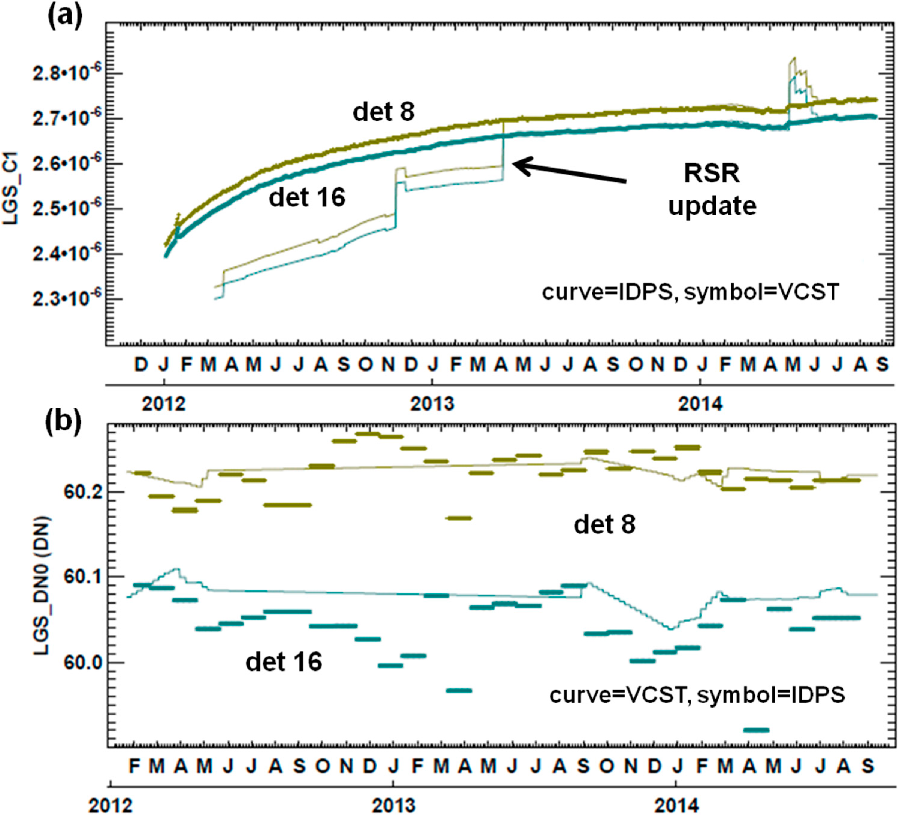
The trending for the LGS gain (
Figure 5a) shows that the gain has gradually increased over time due to the RTA mirror darkening and the spectral shifts in the DNB sensor’s RSR. Except for a short period before the DNB sensor reached operational temperature (20 January 2012) and its gradually increasing trend, the gain appears quite stable over time. In comparison, the IDPS gains are very close to our LGS gains after the April 2013, RSR update. Before the update, the IDPS gains are lower and have several jumps. The discontinuities in the IDPS gains show the evolution of DNB offline calibration methodology. Each time an improvement is made in the calibration methodology, a discontinuity in the absolute radiometric gain is often unavoidable. Such updates are not likely to affect imagery quality, as gains for all detectors and gain modes are shifted proportionally. After the RSR update, a sudden jump in IDPS gain can be seen from May to June of 2014. A solar eclipse during SD calibration event was likely the cause of the jump in the gain. The data points affected by the solar eclipse are removed in our LGS gain history file during the QA process because solar irradiance measurements made during a solar eclipse are invalid for the purposes of calibration. The LGS offset trending (
Figure 5b) indicates that there is virtually no drift over time. Our LGS offsets are consistent with IDPS LGS offsets, indicating that the offset drift observed in the calibrator are the same as that observed from the EV. Note that the IDPS offsets are constant within a month, because they are updated once a month from the VROPs.
Figure 5.
Comparison of daily averaged LGS gain and offset values between NASA and IDPS. (a) LGS gain coefficients (LGS_C1), in units of W∙cm−2∙sr−1; (b) LGS offset (LGS_DN0) in digital numbers (DNs). The plots show aggregation Mode 1, Detectors 8 and 16 as an example. VCST, VIIRS Characterization Support Team.
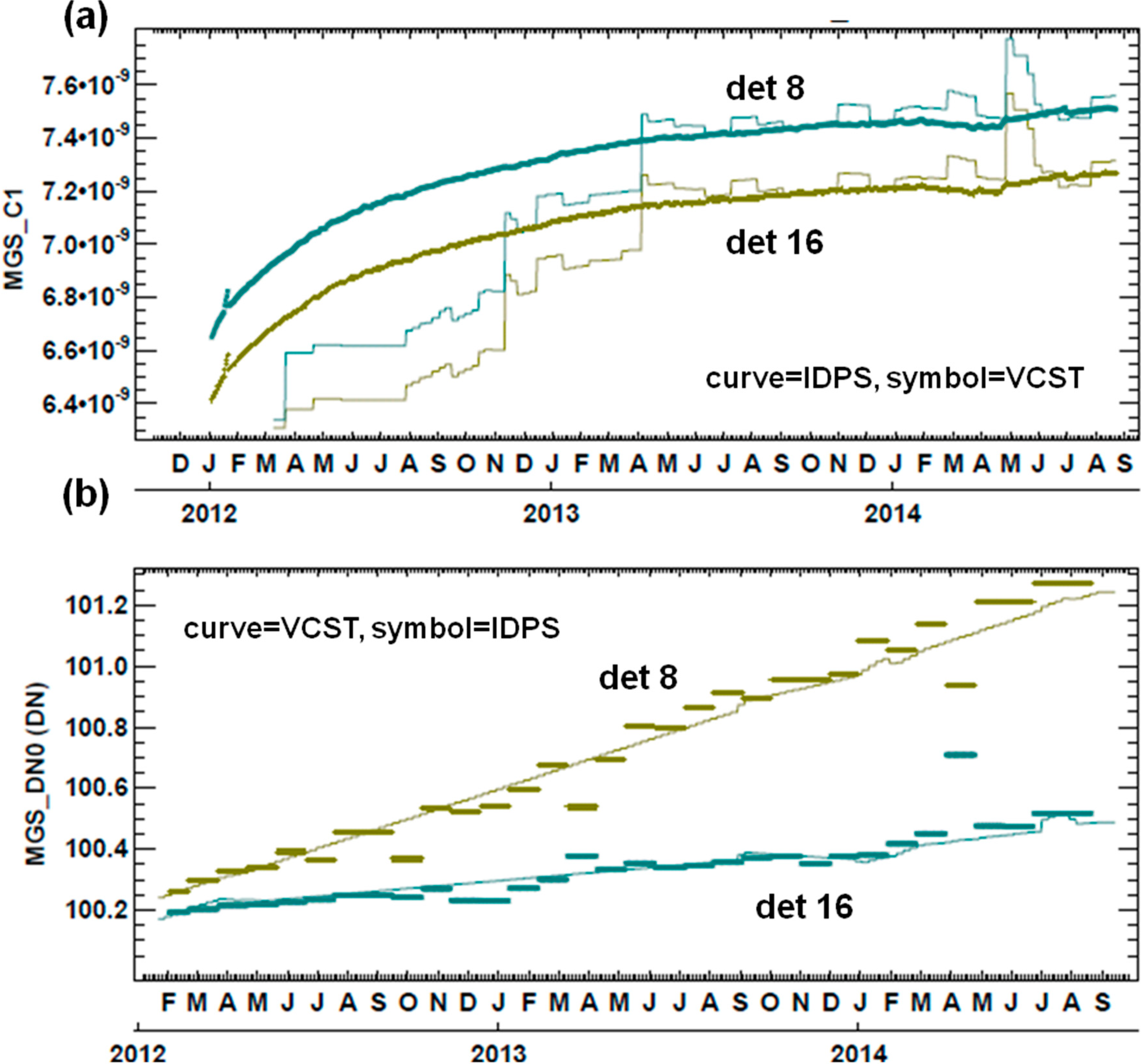
Figure 6.
Comparison of daily averaged MGS gain and offset values between NASA and IDPS. (a) MGS gain coefficients (MGS_C1), in units of W∙cm−2∙sr−1; (b) MGS offset (MGS_DN0) in DNs. The plots show aggregation Mode 1, Detectors 8 and 16 as an example.
Figure 6.
Comparison of daily averaged MGS gain and offset values between NASA and IDPS. (a) MGS gain coefficients (MGS_C1), in units of W∙cm−2∙sr−1; (b) MGS offset (MGS_DN0) in DNs. The plots show aggregation Mode 1, Detectors 8 and 16 as an example.
The MGS gain trending (
Figure 6a) shows a gradual increase over time that is similar to what was observed in the LGS gain trending. Since MGS gain is computed from LGS gain and MGS/LGS gain ratios, the results indicate that the MGS/LGS gain ratios have remained relatively constant over time [
8]. The IDPS MGS gains show a general trend that is similar to IDPS LGS gain with additional monthly fluctuation. Despite the monthly fluctuation, IDPS MGS gains are fairly consistent with our results after the RSR update (April 2013), except for the spurious LGS gains during May to June of 2014. The monthly discontinuity is caused by the monthly update in MGS/LGS gain ratio tables. It has been suggested that the stray light could pose challenges in determining gain ratios using either SD data (our method) and the Earth scene data (IDPS method) [
8,
20]. Although it is difficult to verify, we believe that a gradual and predicable MGS gain drift over time should be more accurate. The MGS offset trending (
Figure 6b) shows a very slow increase of about 0.4 digital number (DN) counts per year. The IDPS MGS offsets track our values very well despite the fact that they are only updated once a month.
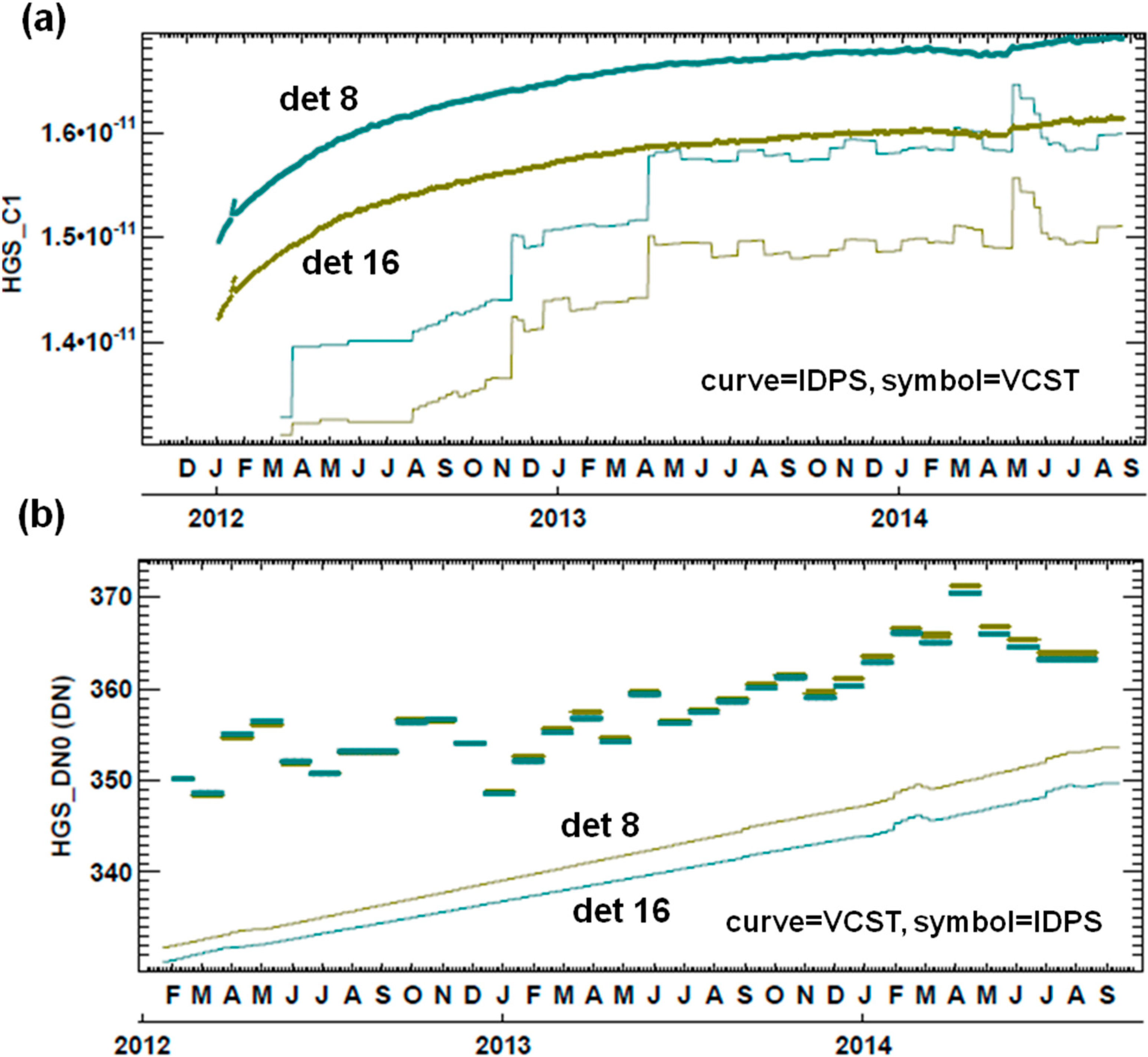
Figure 7.
Comparison of daily average HGS gain and offset values between NASA and IDPS. (a) HGS gain coefficients (HGS_C1), in units of W∙cm−2∙sr−1; (b) HGS offset (HGS_DN0) in DNs. The plots show aggregation Mode 1, Detectors 8 and 16 as an example.
Figure 7.
Comparison of daily average HGS gain and offset values between NASA and IDPS. (a) HGS gain coefficients (HGS_C1), in units of W∙cm−2∙sr−1; (b) HGS offset (HGS_DN0) in DNs. The plots show aggregation Mode 1, Detectors 8 and 16 as an example.
The HGS gain (
Figure 7a) also follows a general upward trend similar to the MGS and LGS gains, but with some small fluctuations over time. The IDPS HGS gains show a trend that is similar to its MGS gains, where discontinuities are apparent due to the monthly gain ratio updates. After the RSR updates, our HGS gains are about 6%–7% higher than those in the IDPS LUT. The differences are attributable mainly to the HGS/MGS gain ratios, since the MGS gains of the two calibration products are very similar. Studies have suggested the disproportionate levels of stray light on the MGS and HGS detectors during cross-stage calibration as the possible cause of this discrepancy [
8,
20]. More research is needed for future improvement in HGS gain accuracy. The HGS offset (
Figure 7b) shows a gradually increasing trend over time of about six DN per year. The monthly updated IDPS HGS offsets are higher and appear to fluctuate over time, while having the same general upward trend as our HGS offset trends. Since our HGS offset is trended by BB observations and from deep space scenes recorded during an S-NPP pitch maneuver, both of which are free of airglow, the HGS offset comparison may indicate the variation in airglow intensity during each month’s offset determination.
The gain and offset comparisons highlight the progress acquired in our knowledge of how to best calibrate the ultra-sensitive DNB sensor on S-NPP VIIRS. It shows the advantage of using the pitch maneuver and BB observations to determine HGS offset and the impact of the modulated RSR on the gain. It also indicates the need for further research on improving gain determination, especially for the HGS, which is used for most of the nighttime observations. Finally, the results show the need for reprocessing using calibration coefficients generated based on the most updated method if consistent data are desired.
3.4. SNR and White Noise
White noise and signal-to-noise ratio (SNR) estimates derived from statistical analyses of DNB calibration data are characterized and trended to monitor the DNB performance. The DNB sensor collects 15 usable samples for each calibration sector for all four gain stages (HGA, HGB, MGS and LGS). It is assumed that the signals are stationary during the very short 15-sample collection time (approximately 2 ms, depending on aggregation mode). Because the DNB calibration view offsets are sample dependent, the sample offset patterns need to be determined before the noise can be estimated from the sample variance.
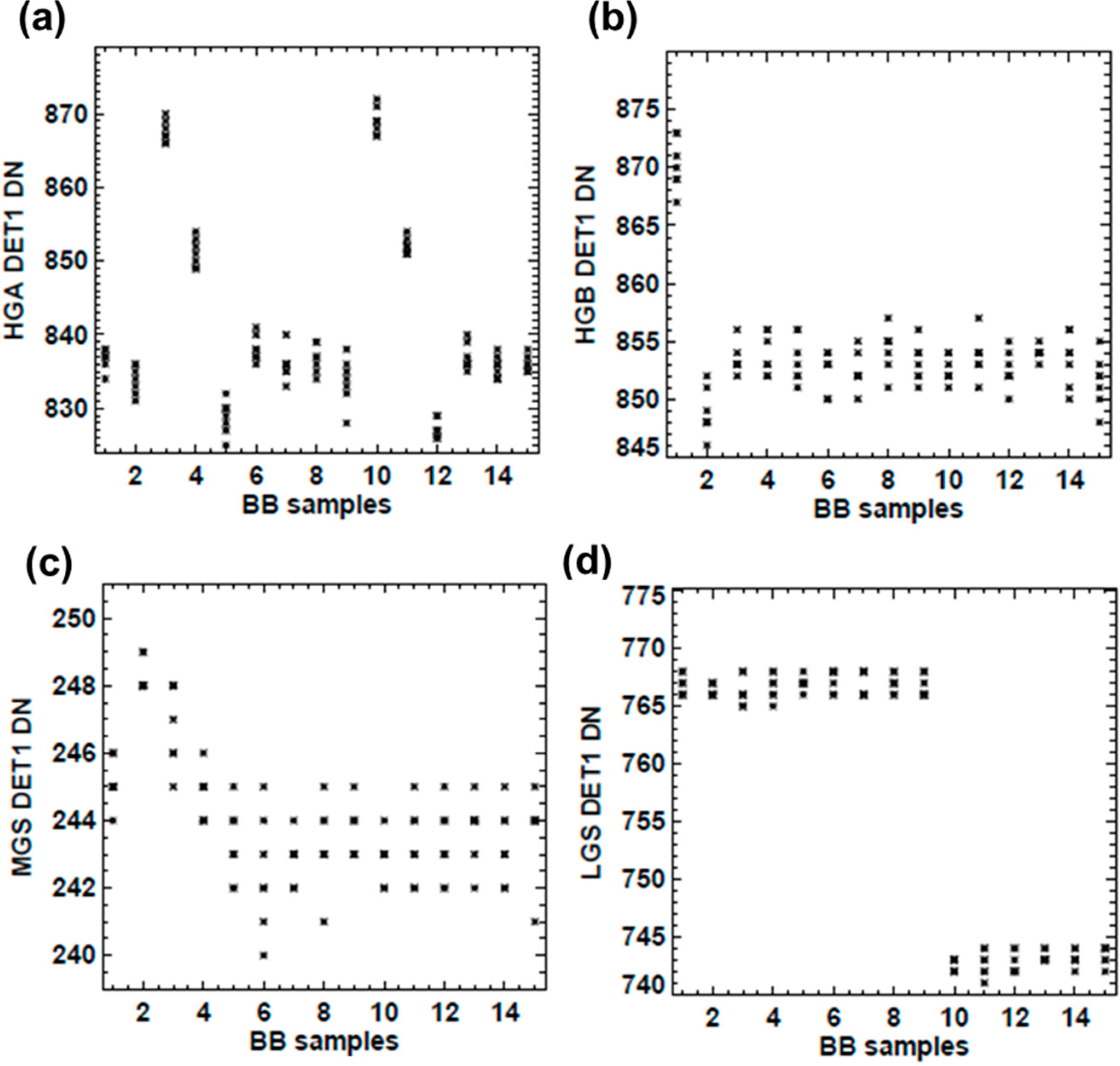
Figure 8 shows an example of a dark offset pattern generated via data collected from successive dark scans. This offset pattern is caused by a limitation in the DNB sensor’s electronics timing card and varies by detector, gain stage and aggregation mode, but is independent of calibration view and the half-angle-mirror (HAM) side. Computing sample noise without removing this fixed pattern will result in artificially increased noise estimates.
Figure 8.
Repeat DNB measurement of DN at each BB sample during orbit 6600 (4 February 2013, 13:23 UTC) when the spacecraft is on the dark side of the Earth. HGA, HGB, MGS and LGS are shown from (a) to (d). The repeated dark measurements show a fixed pattern behavior that is different across gain stages. The plots show aggregation Mode 26, Detector 1 as an example, and the fixed pattern is different at different aggregation modes and detectors.
Before computing the sample variance, the DNB calibration view dark offset sample patterns are determined from data collected from the BB while the spacecraft is within the Earth’s shadow. The offset sample patterns are determined for a given day for each detector, gain stage and aggregation mode. Using the estimated calibration view sample offsets, we can compute the background subtracted DN for each DNB calibration view sample. We then compute the DNB noise from the variance of the 15 calibration view samples. The noise is computed as the sample standard deviation of the zero radiance view, and the SNR is computed assuming a mean view radiance of 3 × 10⁻⁹ W∙cm−2∙sr−1, the specified minimum DNB dynamic range.
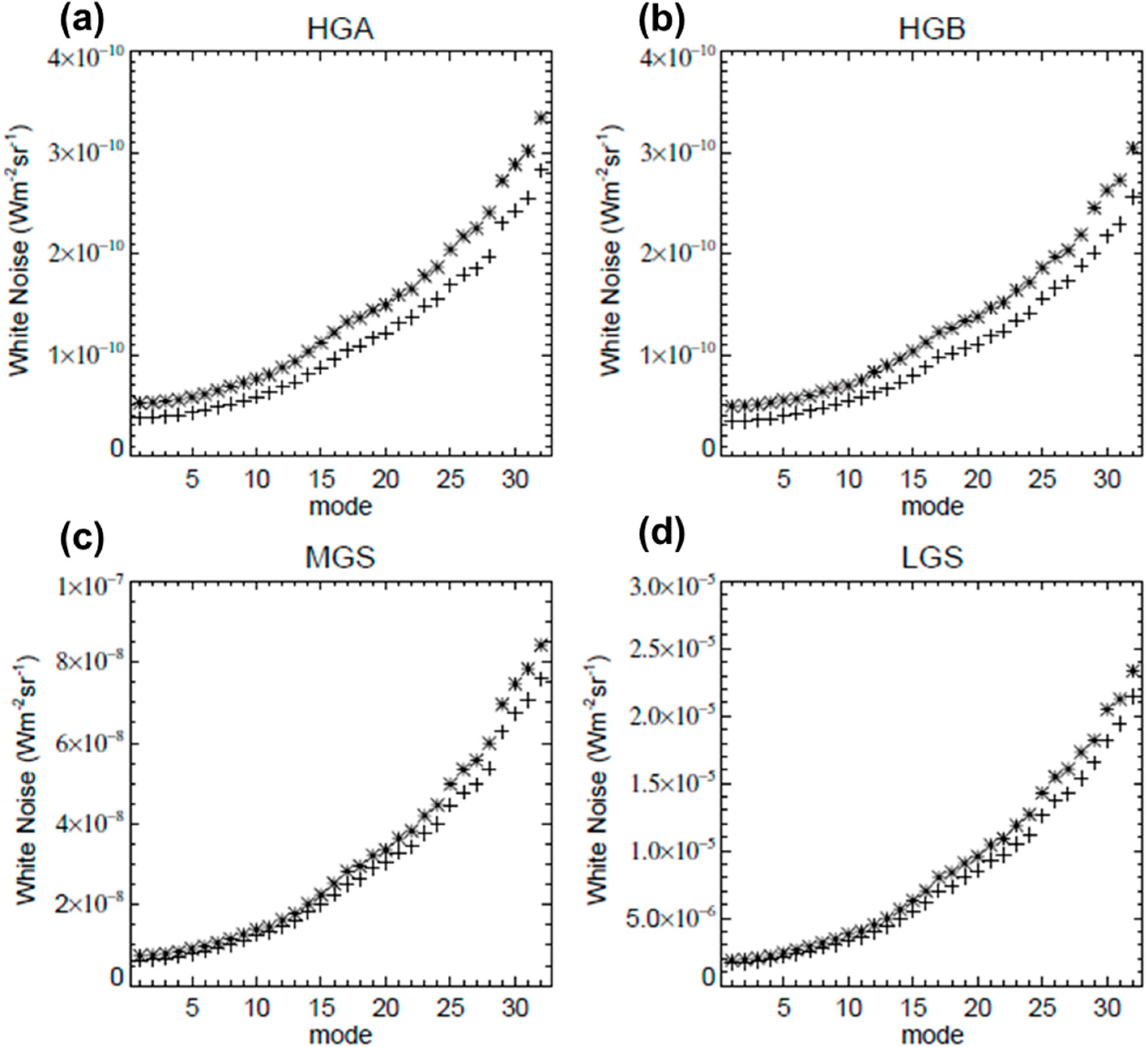
Figure 9 shows the detector-averaged DNB white noise computed using BB dark views for all gain stages and aggregation modes.
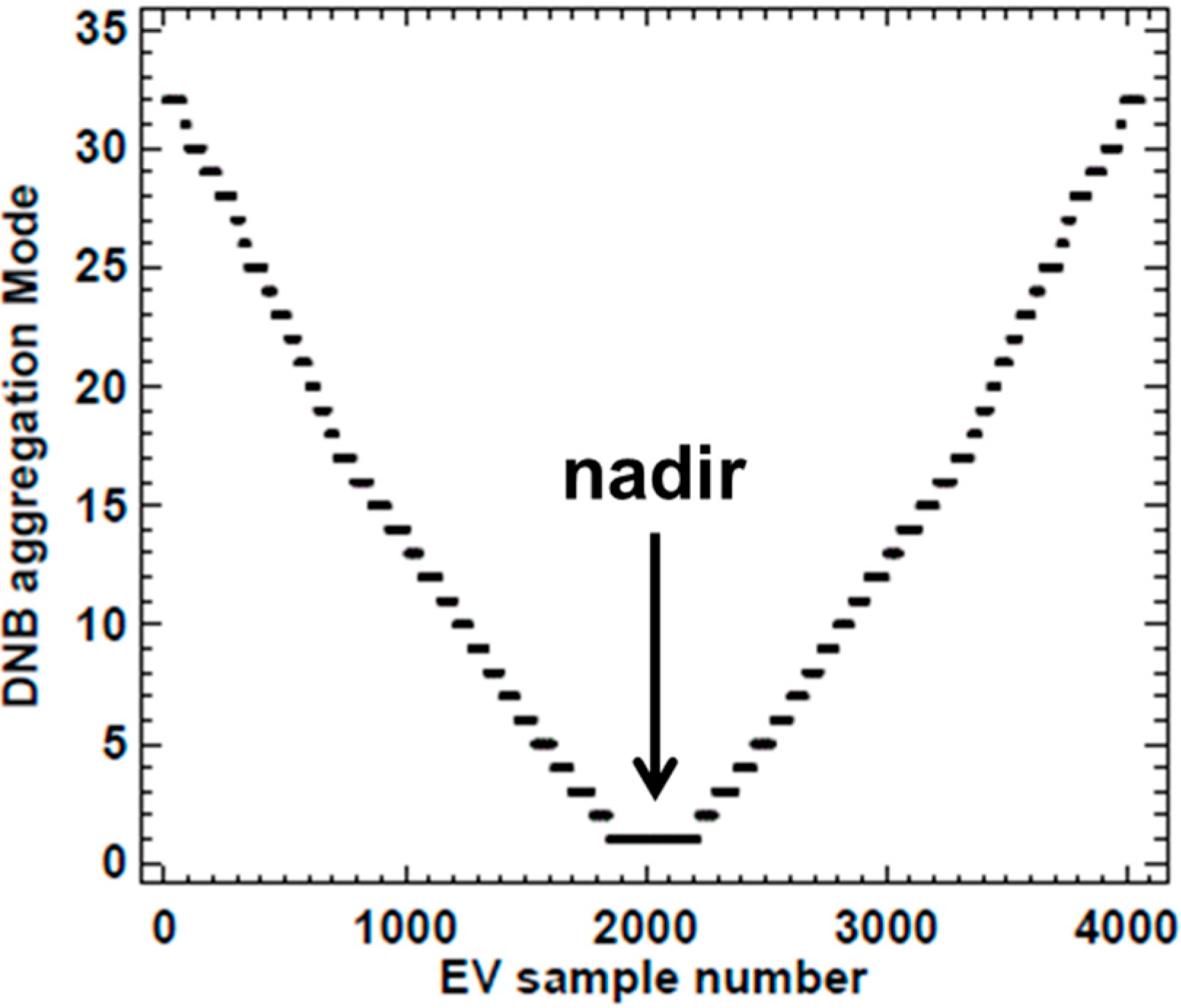
Figure 10 shows the DNB aggregation mode used for each set of EV samples. The information in
Figure 9 and
Figure 10 gives an estimate of white noise at each EV sample. The mean values for the months February 2012, and August 2014, are shown as (+) and (*), respectively, in the plots. The DNB white noise has slowly increased over time (results not shown here), and we show the 2012 and 2014 values as snapshots. For white noise in a specific time frame, it is reasonable to interpolate the values from the 2012 and 2014 values. The white noise is lower at the lower aggregation modes near the nadir EV scan angle and gradually increases toward higher aggregation modes near the edge of the EV scan. The redundant high gain stages, HGA and HGB, have similar white noise profiles and increasing trends over time. The white noise measured for the HGA/HGB detectors are ~0.4 × 10
−10 to ~3 × 10
−10 W∙cm
−2∙sr
−1 from Modes 1 to 32 (nadir to the edge of EV scan) indicating a noise floor that is at least an order of magnitude lower than the design dynamic range (3 × 10
−9 W∙cm
−2∙ sr
−1). The MGS white noise is ~0.7 × 10
−8 to ~8 × 10
−8 W∙cm
−2∙sr
−1, and the LGS white noise is ~0.2 × 10
−5 to ~2.3 × 10
−5 W∙cm
−2∙sr
−1 from the center to the edge of the EV scan. Both MGS and LGS white noise also increased over time, although at a slower rate than the HGA and HGB noise.
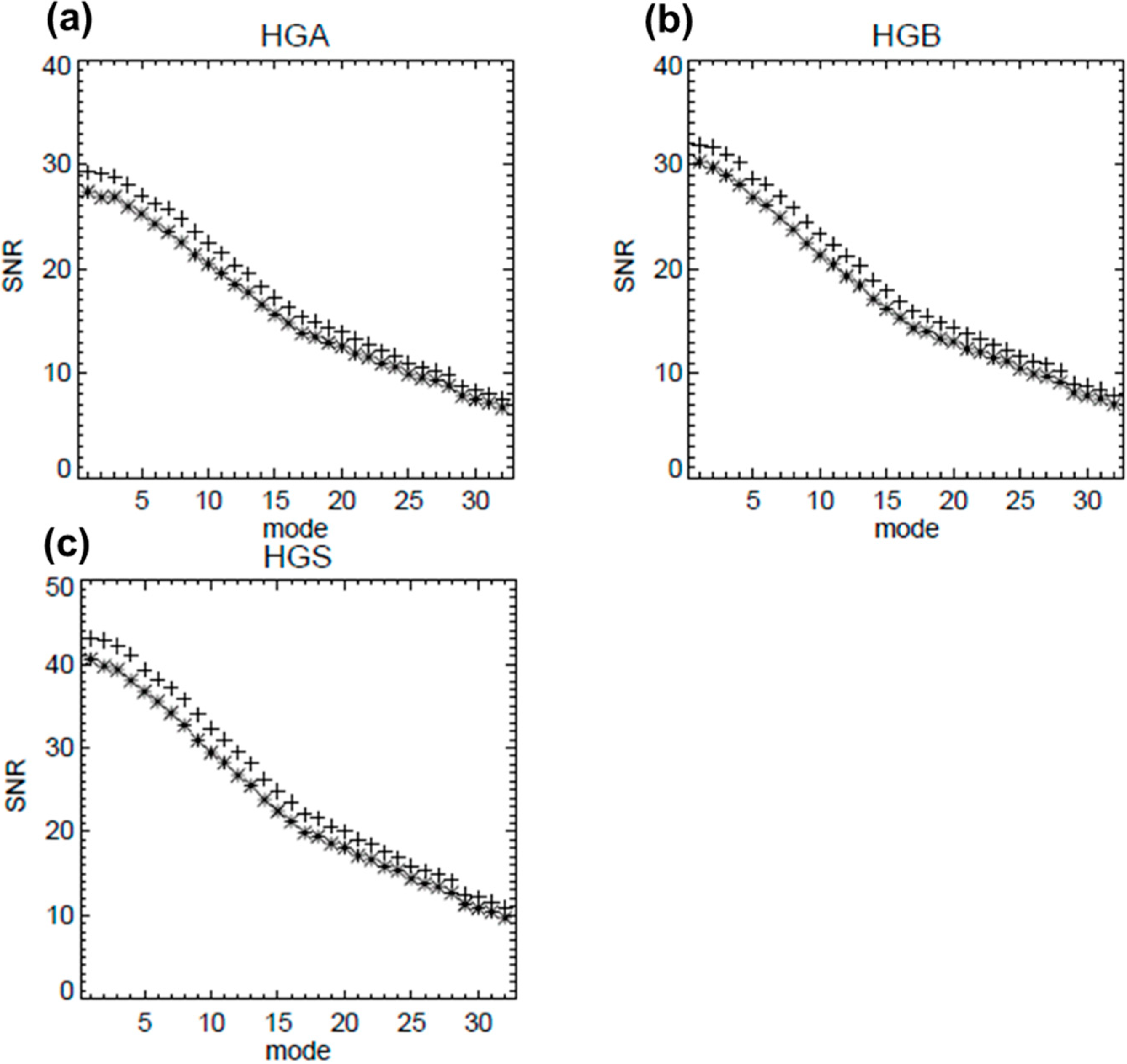
Figure 11 shows the detector-averaged SNR for the HGA, HGB and HGS. The mean SNR values for the months February 2012, and August 2014, are shown as (+) and (*), respectively, in the plots. The HGA and HGB SNRs are computed using SV samples when the S-NPP spacecraft is crossing the north-south terminator during the night orbit where the Earth radiance is near the specified SNR radiance of 3 × 10
−9 W∙cm
−2∙sr
−1. Our estimates show that the SNRs for both HGA and HGB have slowly decreased over time (results not shown here) as indicated by the 2012 and 2014 values. HGA and HGB SNRs decreased at similar rates over time with the lower aggregation modes having slightly larger decreases. The decrease in SNR is expected and is mostly caused by the decrease in detector gain due to RTA mirror darkening [
15] and the increase in detector noise over time. Since the DNB’s EV high gain stage (HGS) readout is the average of HGA and HGB data, the HGS SNR will be higher than the individual HGA and HGB stages [
14]. Because the HGA and HGB data are reported separately in the calibration view, the HGS SNRs were estimated using a standard noise propagation method (Equation (2)):
Figure 9.
Detector averaged white noise computed from BB view data during February 2012 (+), and August 2014 (*). HGA, HGB, MGS and LGS are shown from (
a) to (
d), respectively. The x-axis indicates the DNB aggregation modes, where Modes 1 to 32 are used to collect data from nadir to the edge of the scan (see
Figure 10).
Figure 10.
DNB aggregation modes vs. EV samples. The entire DNB EV consists of 4064 samples from the edge-to-edge scan angle with Sample 2032 centered at the nadir. A total of 32 aggregation modes are used to cover nadir to the edge of the scan angles, with Mode 1 being a nadir mode and Mode 32 at the edge of the scan. The FOV varies among aggregation modes, with Mode 1 being the largest FOV and Mode 32 being the smallest in order to provide near-consistent ground resolution.
The estimated HGS SNRs represent the nominal EV high gain radiometric sensitivity where HGA and HGB data are averaged to produce HGS data.
Figure 11 shows that the HGS SNRs are above 40 in the most sensitive nadir aggregation Mode 1 and monotonically decrease to ~10 at the edge aggregation Mode 32. This large change in HGS SNR is due to varying DNB CCD sub-pixel aggregation to achieve the near-constant ground resolution. The minimum usable radiance, therefore, is dependent on scan angle and is much lower than the design specification at nadir. In summary, the DNB data quality is much better at nadir than the edge of the scan. Users should take notice of this characteristic to make full use of DNB data.
Figure 11.
Detector averaged SNR computed from SV view data for February 2012 (+) and August 2014 (*). HGA, HGB and HGS are shown from (
a) to (
c). The x-axis indicates the DNB aggregation modes, where Modes 1 to 32 are used to collect data from nadir to the edge of the EV scan (see
Figure 10).
Figure 11.
Detector averaged SNR computed from SV view data for February 2012 (+) and August 2014 (*). HGA, HGB and HGS are shown from (
a) to (
c). The x-axis indicates the DNB aggregation modes, where Modes 1 to 32 are used to collect data from nadir to the edge of the EV scan (see
Figure 10).
3.5. Stray Light Correction
The S-NPP VIIRS DNB on-orbit stray light contamination is larger and wider than was originally expected, with up to 25% of all nighttime data affected. The stray light is caused by the sneak path radiance when the S-NPP spacecraft is illuminated by the Sun and is most prominent while the Earth remains dark. The stray light affects regions covering high latitudes of the Northern and Southern Hemispheres. The magnitude of stray light and the affected latitudes are time dependent, as they are determined by the Earth-Sun-spacecraft geometry. The stray light magnitude also varies by detector, HAM mirror side and RTA position (or scan angle), as the sneak path is different for each detector and can be modified by HAM mirror and RTA position. A correction algorithm was developed by the IDPS SDR team to estimate the stray light at each new moon [
11], and a stray light correction LUT was generated to be incorporated in the DNB SDR calibration algorithm to remove excess stray light. The stray light correction was implemented in the IDPS operational process in August 2013. Because IDPS only performs forward processing, the DNB SDRs prior to August 2013, do not have stray light correction applied. Furthermore, the IDPS operational DNB SDR is generated by using the previous month’s stray light correction LUT due to the offline processing latency normally required to apply the new correction LUT into the operational data stream. To remove such a latency constraint, the IDPS has started to apply stray light correction LUTs generated for the same month from the prior year. The updated strategy improves the correction accuracy as the stray light pattern repeats for the yearly Earth-Sun-spacecraft geometry cycle. However, some biases still exist when using the prior year’s stray light estimate for correction.
At NASA, we have developed our own stray light correction method and have generated mission-wide stray light correction LUTs. These LUTs were used in Land PEATE Collection 1.1 reprocessing. The NASA DNB stray light correction method is based on the same principles as used in the IDPS method [
11], which assumes that the small signal observed over the dark Earth scene during a new moon is the result of a combination of stray light and airglow [
21]. Our method, however, is different than the IDPS method in two ways. First, the dark Earth scene signals are computed from up to 14 orbits (one full day) of data during the new moon period, as opposed to the IDPS method, which uses an Earth nighttime light map to mask out the nightlight [
11]. In our method, pixels with nightlight are removed as outliers, because repeat measurements at each successive orbit will cover different parts of the Earth. Since nightlights are present in only a small fraction of the Earth’s surface, a carefully-selected outlier exclusion threshold can remove most of the contaminated pixels. Secondly, the computed dark scene signals are smoothed over the spacecraft zenith angle and scan angles, except for the region with high contrast,
i.e., the penumbra region. In twilight regions, where the Earth scene signals increase exponentially, stray light is assumed to be the same as the last known value as an approximation. Lastly, the airglow in the dark scene is subtracted from regions not affected by the stray light and is subtracted from the dark signals to generate the final stray light estimates. Although we do not attempt to quantify the uncertainty of the corrected radiance, we estimate it to be about half of the scene’s airglow variation within the same scan angle. This uncertainty is due to the averaging, smoothing and airglow estimates derived from a region that is likely to have different airglow than the regions affected by stray light.
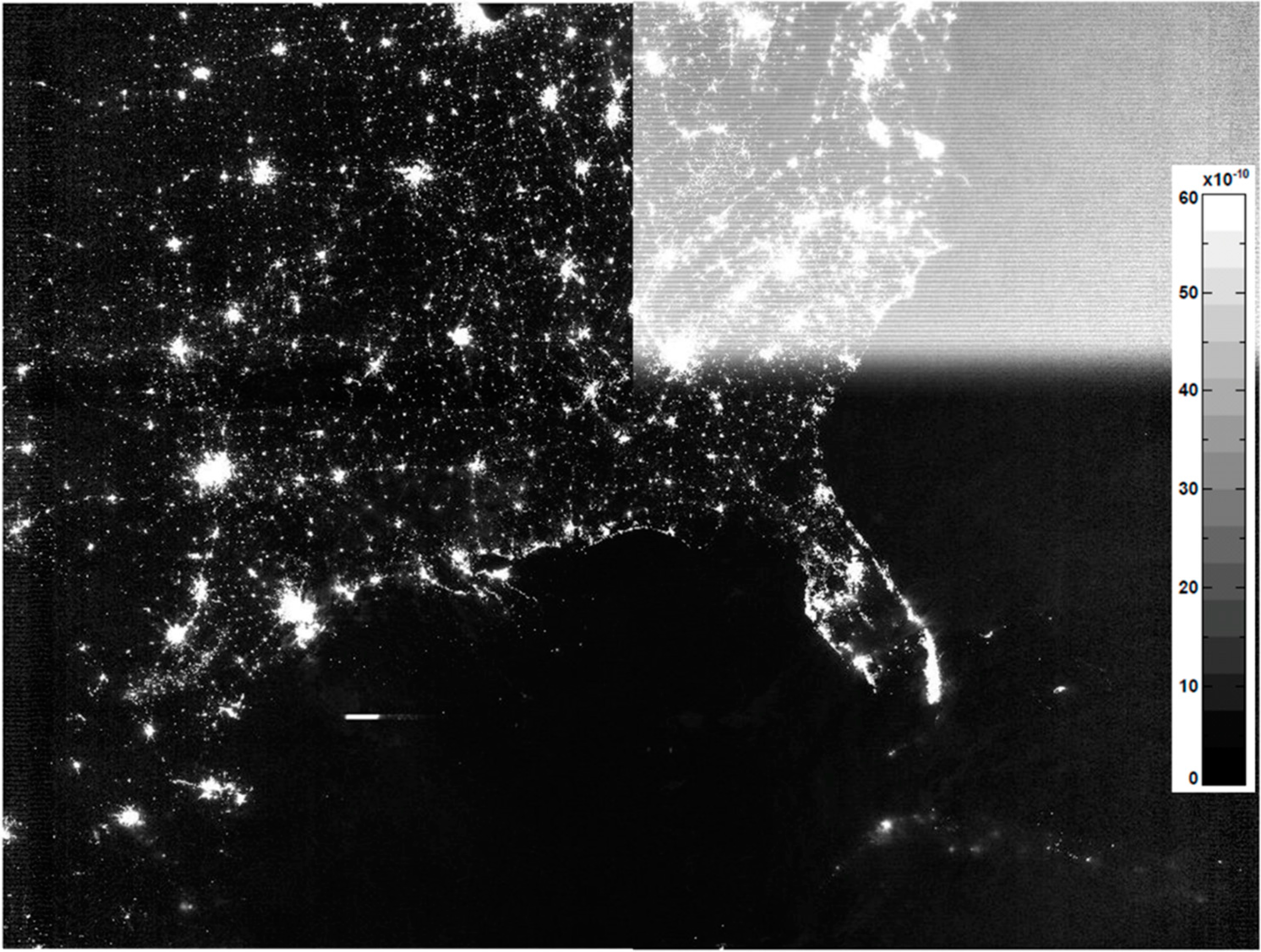
Figure 12 shows an example of a North America DNB SDR image before and after stray light correction. Before the correction (right side of the image), the stray light is visible everywhere north of South Carolina of the United States of America. The apparent striping in the image is the result of strong stray light detector dependency. After the correction (left side of the image), the image is free from stray light contamination without any visible quality degradation of real nightlight features. Note that the latitude of the stray light affected region will change over time as it depends on the Earth-Sun-spacecraft geometry. Because the Earth-Sun-spacecraft geometry roughly repeats at a yearly cycle, the stray light pattern will follow the same cycle. Because of this yearly cycle, it might be a good approximation to use the prior year’s stray light correction LUT generated for the same month [
21]. However, retroactive verification is necessary, because factors, such as spacecraft altitude, attitude, declination angle drift,
etc., might not follow the yearly cycle.
Figure 12.
An example of Northern Hemisphere DNB SDR image before and after applying stray light correction. The image was taken on 19 June 2012, 07:27 UTC. The legend is in units of W∙cm−2∙sr−1.
Figure 12.
An example of Northern Hemisphere DNB SDR image before and after applying stray light correction. The image was taken on 19 June 2012, 07:27 UTC. The legend is in units of W∙cm−2∙sr−1.
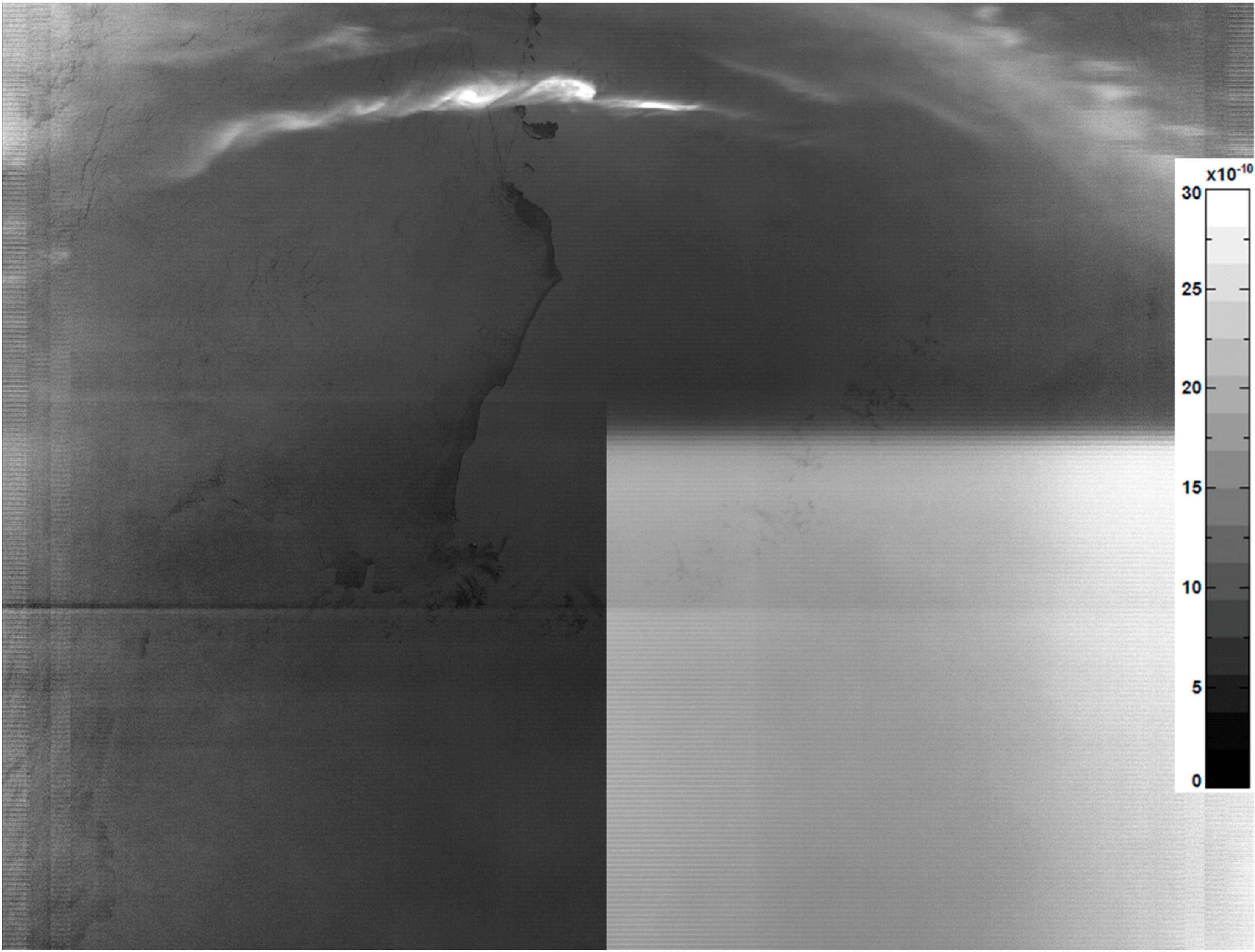
Figure 13 shows another stray light correction example in the Southern Hemisphere. The uncorrected part of the image (right side in
Figure 13) showed that the stray light has a two-tone pattern, which is the result of additional stray light entering through the SD screen, a path that is only possible when the spacecraft is near solar calibration events in the southern day-night terminator crossing. Removing the stray light from the SD path is challenging, because it is more sensitive to the spacecraft azimuth angle than the stray light entering from the EV port. The stray light corrected part of the image (left side in
Figure 13) shows that most of the stray light-associated features are removed. However, a dark strip can be observed about 2/3 down in the image that is the result of over-correction. The over-correction is mostly caused by the drift of the SD port stray light onset angle since the stray light correction LUT was generated. The accuracy of the SD port stray light onset angle is important, because the stray light signal has a sharp increase. The mismatched SD port stray light onset angle will result in either over- (in
Figure 13 example) or under-correction. Because the SD port stray light onset angle changes at a faster rate than the onset of EV port stray light angle, using the stray light correction LUT derived from the closest new moon data can minimize the SD onset angle differences. In verifying the SD onset angle shifts, we generated test images using stray light correction LUTs from prior months (results not shown here). We found that the area of under-correction increases as the time between the image and correction LUT time. For future improvement, a new LUT format or a different approach is needed to remove the limitations of the current design of the stray light correction mechanism.
Figure 13.
An example of Southern Hemisphere DNB SDR product before and after applying stray light correction. The image was taken on 19 June 2012, 08:01 UTC. The legend is in units of W∙cm−2∙sr−1.
Figure 13.
An example of Southern Hemisphere DNB SDR product before and after applying stray light correction. The image was taken on 19 June 2012, 08:01 UTC. The legend is in units of W∙cm−2∙sr−1.


