Hydrological Impacts of Urbanization of Two Catchments in Harare, Zimbabwe

Abstract

By increased rural-urban migration in many African countries, the assessment of changes in catchment hydrologic responses due to urbanization is critical for water resource planning and management. This paper assesses hydrological impacts of urbanization on two medium-sized Zimbabwean catchments (Mukuvisi and Marimba) for which changes in land cover by urbanization were determined through Landsat Thematic Mapper (TM) images for the years 1986, 1994 and 2008. Impact assessments were done through hydrological modeling by a topographically driven rainfall-runoff model (TOPMODEL). A satellite remote sensing based ASTER 30 metre Digital Elevation Model (DEM) was used to compute the Topographic Index distribution, which is a key input to the model. Results of land cover classification indicated that urban areas increased by more than 600 % in the Mukuvisi catchment and by more than 200 % in the Marimba catchment between 1986 and 2008. Woodlands decreased by more than 40% with a greater decrease in Marimba than Mukuvisi catchment. Simulations using TOPMODEL in Marimba and Mukuvisi catchments indicated streamflow increases of 84.8 % and 73.6 %, respectively, from 1980 to 2010. These increases coincided with decreases in woodlands and increases in urban areas for the same period. The use of satellite remote sensing data to observe urbanization trends in semi-arid catchments and to represent catchment land surface characteristics proved to be effective for rainfall-runoff modeling. Findings of this study are of relevance for many African cities, which are experiencing rapid urbanization but often lack planning and design.

1. Introduction

Understanding the impacts of land conversion and land cover changes on the hydrological cycle has become a global concern in view of the increasing urban populations [1,2]. Studies by [3,4] concluded that the effects of land conversions on river flows are of major interest to water resource managers and hydrologists as they plan, manage and develop water resources. [5] observed that increases in impervious areas through urbanization may result in the following hydrological impacts (i) reduced interception by tree canopies; (ii) reduced infiltration; (iii) increased surface runoff; (iv) increased flow velocities in urban areas due to decreased surface roughness and (v) increased peak flow discharges. Similarly, [6] noted that conversion of natural catchments to peri-urban or urban areas affect many processes of the hydrological cycle, such as interception, infiltration, evaporation and streamflow by runoff processes. However, the magnitude of impacts of urbanization on hydrological processes is commonly not well known especially in large parts of Africa. Furthermore, conclusive studies on the implications of urbanization on closure of the water balance and availability of water resources are limited [5,7,8,9]. Yet knowledge on the effects of urbanization on the hydrology of catchments is critical for water resources management in most water-scarce areas, such as those in Africa.

Studies that have assessed impacts of urbanization have adopted different approaches. For instance, [10] studied the effects of suburban developments on runoff generation using hydrograph analysis techniques. They showed that with increased suburban development there was an accelerated recession phase and increased peak flows. Similarly, [11] analyzed hydrograph characteristics at an annual scale for a 38-year runoff record to determine the effects of urbanization on streamflow. The study showed that the annual runoff coefficient of the urban stream (Peachtree Creek) was not significantly greater than that of the less-urbanized watersheds. However, the storm recession period of the urban stream was one to two days less than that of the other streams. [12] applied a water budget and meteorological approach to assess the effects of urbanization on catchment evapotranspiration (ET). The study showed significant decreases in catchment ET that were linked to increases in urban and residential areas. In a different study, [13] assessed the impacts of urbanization of river flow frequencies by a controlled experimental modeling approach using the model MIKE-SHE and the 1D hydrodynamic river model MIKE-11. The study showed that the frequency of low flows decreased with increasing urban expansion and that the frequency of average and high-flow events increased with increasing urbanization. Recently, there have been attempts to incorporate remote sensing data in hydrological models to enhance understanding of the effects of urbanization on the hydrological cycle. [14] applied a coupled distributed Hydrologic Engineering Center’s Hydrologic Modeling System (HEC-HMS) for runoff simulations with the integrated Markov Chain and Cellular Automata model (CA-Markov model) for development of future land use scenario maps. Landsat and CBERS satellite data were used. The results showed that increases in annual runoff volume, daily peak flows and flood volume between the years 1988–2009 could be related to urbanization. These hydrological variables were projected to further increase with increasing urbanization. These studies have encouraged incorporation of land use change information in distributed hydrologic models. However, the assessment of urbanization on hydrological impacts of catchments remains complicated due the spatial heterogeneity of the land surface in urban areas (see [5,7]). In this regard, satellite remote sensing provides an opportunity to assess and track changes in land cover over selected space and time domains thereby serving as an important input in impact assessments and modeling studies. Despite the importance of remote sensing in providing land cover maps which are critical inputs to hydrological models, there are often inconsistencies that may arise from image misclassifications or registration errors [15]. It is therefore important to correct for such inconsistencies through assessment of land use and land cover (LULC) spatial and temporal patterns [15,16] and or through accuracy assessment of classified images [17].

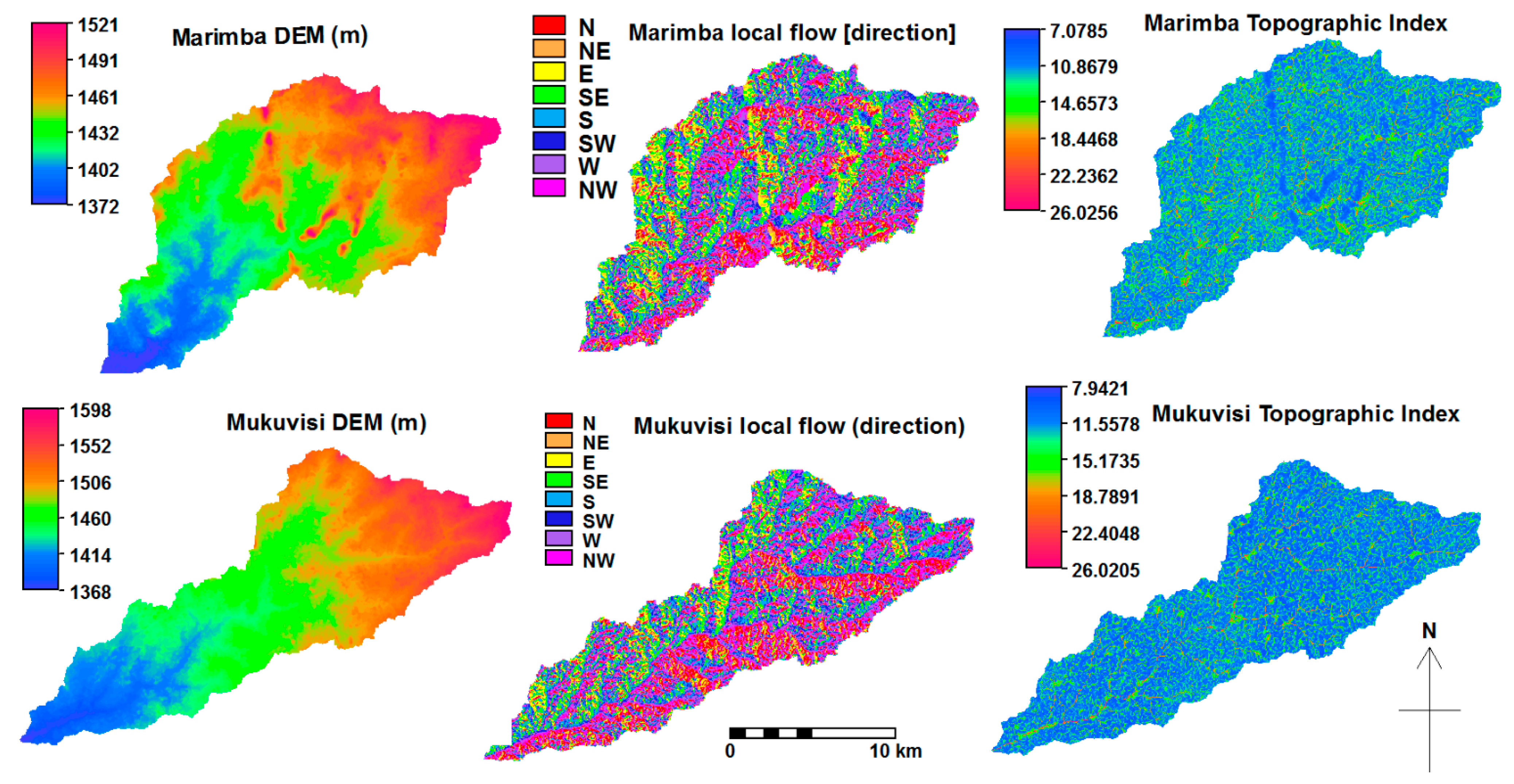
This study relied on satellite remote sensing data to represent land cover and elevation characteristics as inputs for the topographically driven TOPMODEL, which served to simulate the relationship between rainfall and runoff. TOPMODEL is a semi-distributed, mass conservative model which relies on a simple representation of basin characteristics and hydrologic processes [18] as compared to fully distributed and data demanding models like MIKE SHE [19]. The semi-distributed form of TOPMODEL makes full use of elevation data which is freely available through the Advanced Spaceborne Thermal Emission and Reflection Radiometer (ASTER) or the Shuttle Radar Topography Mission (SRTM) Digital Elevation Models (DEMs). TOPMODEL requires a small number of topographic and land surface based parameters and makes optimized parameter values physically meaningful [20]. Furthermore, in its setup, the model can adapt to a specific catchment and specific modeling purposes [21]. However, TOPMODEL mostly has applications in natural catchments [22,23,24,25,26] with only few applications in urban catchments [6,27]. Latter applications have characterized urbanized land cover by introducing impervious surfaces with very low percolation and surface infiltration rates [6,9,23,28] which resulted in increased and more rapid runoff responses. Despite these efforts, the use of TOPMODEL approach in an urban setting as shown in [6] indicated that the ISBA-TOPMODEL simulations underestimated total streamflow during dry periods whereas it overestimates streamflow during rain events and wet weather conditions. In the study by [29], modifications of TOPMODEL (TOPURBAN v.1 and v.2) were tested for urbanized watersheds by altering the topographic index and the mechanism to generate surface runoff but detailed descriptions on the processing of data including remote sensing data were missing. In fact, several studies [9,10,11,13,14] that have characterized urbanized land cover types for hydrological assessments have failed to adequately capture relevant spatial information of historical land surfaces in urban catchments. In that regard, this study determined historical changes in land cover and incorporated topographical attributes through ASTER DEM hydro-processing approaches as a first step towards assessing impacts of urbanization on hydrology.

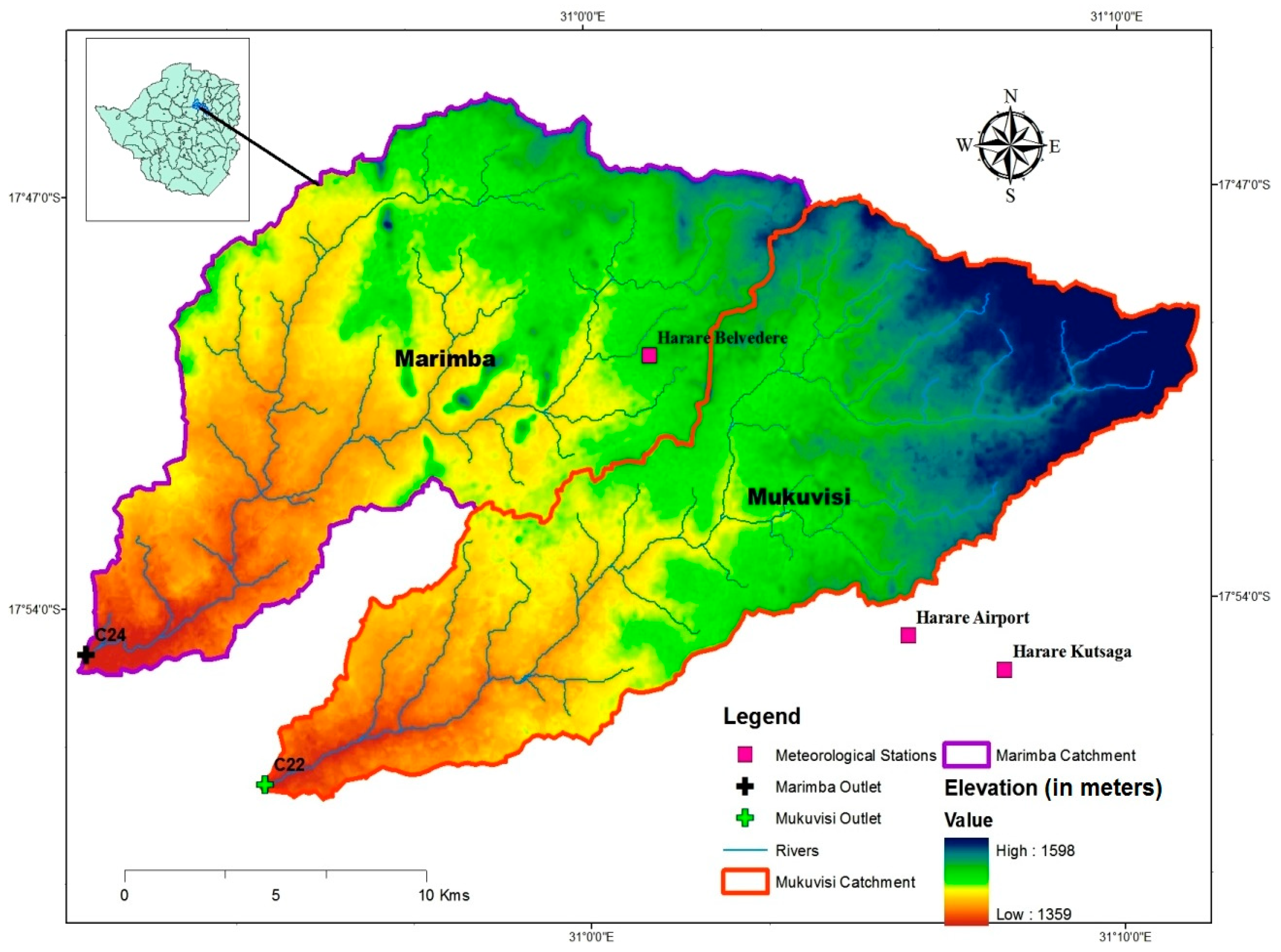
Within the African context, the assessment of the impacts of urbanization on streamflow is important for water development and management. Urbanization in Africa is common due to urban migration resulting in increases in paved and built-up areas in the urban setting. According to [30], Africa is one of the hotspots of serious urban growth and will continue to be so for the next four decades. It is projected that the population of African cities will increase by 0.9 billion by 2050. In Zimbabwe, the population of Harare has grown from 1.8 million in 2002 to 2.1 million in 2012 [31]. As a consequence, the demand for land for housing increased and peri-urban and rural areas have been converted to urban areas. In addition to exterior sprawling, densification is a strategy also being applied to grow the city of Harare. Densification promotes the growth of the city through the construction of buildings on lands previously left as open spaces thus increasing the extent of paved and build-up areas. Densification and sprawling have had the concomitant effect of intensifying urbanization. In Harare City, Marimba and Mukuvisi catchments are two catchments that are experiencing rapid urbanization as characterized by rapid growth and densification. Both catchments constitute the greater part of the built-up environment of the city. These catchments are the most urbanized in Harare City and therefore were selected for this study. The urban areas are characterized by middle-to-low income housing, office complexes and industrial areas. Hydrology and water related studies in and around the Marimba and Mukuvisi catchments have mainly focused on water quality and pollution, evapotranspiration and urban drainage [32,33,34]. Only few studies have focused on hydrology and quantification of water resources [35,36], but within the broader context of the Upper Manyame catchment. Detailed studies on hydrological impacts of urbanization of the catchments are unknown to the authors. Objectives of this study are to: (1) assess trends in rainfall and streamflow; (2) assess changes in land cover in the Marimba and Mukuvisi catchments; and (3) assess hydrological impacts of urbanization and land conversion by rainfall-runoff model simulations.

In Section 2 descriptions of the study area and available data are given including satellite data. Methods used in this study are described in Section 3. Findings of the study are presented and discussed in Section 4. Section 5 gives the conclusions and an outline of the recommendations.

2. Study Area and Data

2.1. Description of Study Area

For this study the Marimba and Mukuvisi River catchments in Harare City are selected which are tributary catchments of the Upper Manyame basin in Zimbabwe (Figure 1). Mukuvisi catchment has an area of 223.1 km² and a longest flow path of 44.7 km whereas Marimba catchment has an area of 220.5 km² and a longest flow path of 38.6 km. Both catchments have similar elevation ranges between 1350 m and 1550 m above mean sea level. The soil is primarily sandy clay loam. The mean annual rainfall for the period 2000–2010 is 810 mm/yr whereas potential evapotranspiration is around 1600 mm/yr. These two catchments were selected for this study since both are characterized by a rapid increase of built-up area and urbanization. The dominant residential housing in both catchments is high to medium density houses with limited space for gardens. The population density in the catchments is around 2.540 people/km² according to [31]. However, there are low-density areas in the northern and eastern parts of the catchments that have spacious gardens. Trees are also kept within the residential stands.

Figure 1. Mukuvisi and Marimba catchments in Zimbabwe showing elevation and locations of meteorological stations and streamflow gauging stations.

Figure 1. Mukuvisi and Marimba catchments in Zimbabwe showing elevation and locations of meteorological stations and streamflow gauging stations.

2.2. Hydro-Meteorological Data

For this study, daily streamflow data for the years 1970 to 2008 for the gauging stations of Marimba and Mukuvisi catchments (C22 and C24, respectively) were made available by the Zimbabwe National Water Authority. Time series of daily meteorological data including rainfall data were acquired from the Meteorological Office of Zimbabwe. Potential Evapotranspiration at daily time step is estimated from the meteorological data using the FAO-Penman Monteith method as outlined in [37].

The relation between rainfall and streamflow was assessed as part of data screening. For rainfall time series data from Airport, Belvedere and Kutsaga rain stations was used whereas for streamflow time series data from gauging stations C22 and C24, for Mukuvisi and Marimba catchments, respectively, was used (see Figure 1). Correlation between time series suggests dependency of streamflow on rainfall in both catchments (Table 1).

Table 1. The significant relationship (p < 0.05) between rainfall and streamflow in the study area. All p values were equal to 0.000.

Rain Station	Streamflow Gauging Station	Correlation R
Airport	C22	0.675
Airport	C24	0.649
Belvedere	C22	0.651
Belvedere	C24	0.656
Kutsaga	C22	0.667
Kutsaga	C24	0.642

Table 1. The significant relationship (p < 0.05) between rainfall and streamflow in the study area. All p values were equal to 0.000.

Rain Station	Streamflow Gauging Station	Correlation R
Airport	C22	0.675
Airport	C24	0.649
Belvedere	C22	0.651
Belvedere	C24	0.656
Kutsaga	C22	0.667
Kutsaga	C24	0.642

2.3. Satellite Data

For estimation of the topographic index an ASTER DEM (30 m resolution) covering the study area was retrieved from the Global ASTER GDEM. For land cover change assessments we used land cover images from Landsat satellites, which were processed in ILWIS open source software. Landsat TM images analyzed in the study (path 170 and row 72) were downloaded from the United States Geological Survey (USGS) Global Visualization Viewer (GLOVIS) for the years 1986, 1994 and 2008, all in the dry month of August. Google Earth imagery of the study area was used to assess the imperviousness of the two catchments.

3. Methodology

3.1. Land Cover by Remote Sensing

Table 2 shows the dates of image acquisition, spatial resolution as well as the bands used for land cover change analysis. The false color composites (5, 4, 3) were used in the classification process because of their ability to enhance image interpretation that ultimately facilitates differentiation of land cover types, such as: grass, woodland, cropped area, aquatic weeds and bare surfaces which are critical for assessing changes in land cover as a result of urbanization.

Table 2. Description of imagery used for land cover classification.

Sensor	Date of Acquisition	Spatial Resolution	Bands Used	Cloud Cover
Landsat 5 TM	31 August 1986	30 meters	5, 4, 3	0
Landsat 5 TM	21 August 1994	30 meters	5, 4, 3	0
Landsat 5 TM	10 August 2008	30 meters	5, 4, 3	10 *

^* Although the overall scene had 10% cloud cover, the study site had less than 5% cloud cover.

Table 2. Description of imagery used for land cover classification.

Sensor	Date of Acquisition	Spatial Resolution	Bands Used	Cloud Cover
Landsat 5 TM	31 August 1986	30 meters	5, 4, 3	0
Landsat 5 TM	21 August 1994	30 meters	5, 4, 3	0
Landsat 5 TM	10 August 2008	30 meters	5, 4, 3	10 *

^* Although the overall scene had 10% cloud cover, the study site had less than 5% cloud cover.

Prior to image classification, all the images were georeferenced to the Universal Transverse Mercator zone 36 south projection based on the WGS84 datum. A minimum of 15 ground control points were used during image registration. The nearest neighbour resampling method was used for image registration and a root mean square error less than 0.2 pixels (~6 m) was obtained. To ensure comparability of the images across the years, digital numbers were converted to radiance and from this to a dimensionless top-of-atmosphere (ρTOA) reflectance:

$$\rho TOA=\pi ·L\lambda ·d2/ESUN\lambda ·Cos\theta s$$

(1)

where:

• Lλ = the spectral radiance at the sensor
• d = the Earth-sun distance in astronomical units
• ESUNλ = the mean solar exo-atmospheric irradiance for each band and
• Cosθs = the solar zenith angle in degrees (Irish 1998).

The sensor calibration information, such as solar zenith angle and earth-sun distance, was extracted from the header file of the imagery [38]. Once converted to ρTOA reflectance, bands 5, 4 and 3 representing the Short-wave Infrared, Near Infra-Red and the Red bands of Landsat, respectively, were combined in the ILWIS Geographic Information System (GIS) to create a color composite, which enhanced visualization before image classification. The images were then classified using the maximum likelihood classification algorithm in a GIS environment based on the six land cover classes in the study area (Table 3). The maximum likelihood classification algorithm is based on the probability that a pixel belongs to a particular class and thus a pixel is assigned to a predefined set of classes to which it has the highest probability of belonging to [17]. The maximum likelihood was used for the study because of its robustness [39]. Image classification was important in the determination of land cover, an important determinant of streamflow generation in hydrological catchments. Table 3 provides a description of the classes used in this study.

Table 3. Description of the land cover classes used in the study.

Class	Description
Aquatic weeds	Area under aquatic weeds
Cropped Field	Area under crops
Grassland	Area predominantly covered with grass for a significant part of the year
Urban	Area covered with bare surfaces that have been cleared for urban developments, impervious surfaces, such as roads and buildings
Water	Area occupied by water, such as rivers and wetlands
Woodland	Area covered with sparse to dense woody species, such as shrubs, bushes and trees. Miombo species dominate this cover.

Table 3. Description of the land cover classes used in the study.

Class	Description
Aquatic weeds	Area under aquatic weeds
Cropped Field	Area under crops
Grassland	Area predominantly covered with grass for a significant part of the year
Urban	Area covered with bare surfaces that have been cleared for urban developments, impervious surfaces, such as roads and buildings
Water	Area occupied by water, such as rivers and wetlands
Woodland	Area covered with sparse to dense woody species, such as shrubs, bushes and trees. Miombo species dominate this cover.

Results of classification were assessed for their accuracy using Kappa statistic. The Kappa statistic was based on 1720 ground control points for Marimba catchment and 985 points for Mukuvisi catchment. The ground control points were taken from high resolution Google Earth imagery and aerial photographs for the dates which coincided with the Landsat imagery acquisition dates. The selection of these points was based on the relative proportion of each land cover type derived from visual interpretation of the image. Table 4 shows the average number of these ground control points used for accuracy assessment in the study.

Table 4. Average number of points used for validating the classified landcover images for Marimba and Mukuvisi Catchment.

Land Cover	Marimba	Mukuvisi
Aquatic weed	42	*
Urban	356	322
Cropped Field	128	104
Grassland	678	292
Water	375	89
Woodland	141	178

* No aquatic weeds were observed in Mukuvisi catchment. Aquatic weeds were mainly observed in Lake Chivero.

Table 4. Average number of points used for validating the classified landcover images for Marimba and Mukuvisi Catchment.

Land Cover	Marimba	Mukuvisi
Aquatic weed	42	*
Urban	356	322
Cropped Field	128	104
Grassland	678	292
Water	375	89
Woodland	141	178

* No aquatic weeds were observed in Mukuvisi catchment. Aquatic weeds were mainly observed in Lake Chivero.

After image classification, overlay analysis was performed on the 1986, 1994 and 2008 images to assess land conversion and urbanization in the study area. The result of the overlay analysis is a confusion matrix, which shows land cover and land cover conversions for both catchments for respective years.

3.2. Trend Analysis and Hydro-Meteorological Time Series

Trend analysis for rainfall and streamflow time series is critical to assess if changes in streamflow could be related to changes in rainfall as possibly caused by climate change. In this study, the Mann-Kendall test was used to test whether, statistically, significant trends at monthly and annual base (1954–2006) could be identified. We tested for significant levels at p < 0.05. The Mann-Kendal (MK) test, also known as the as the Kendall’s tau statistic [40,41], is a rank-based non-parametric statistical test that is commonly applied for trend detection [40,42,43]. The test compares the relative magnitudes of sample data rather than the data values themselves [44]. The tau statistic, τ, reads:

$$\tau =\frac{2S}{n(n-1)}$$

(2)

where:

$$S={\displaystyle \sum }_{i-1}^{n-1}{\displaystyle \sum }_{j=i+1}^{n}sign\left(Y_{j-}{X}_i\right)$$

(3)

$$sign\left(Y_{j-}{X}_i\right)=\left(\begin{array}{c}1 if \left(Y_{j-}{X}_i\right)>0\\ 0 if\left(Y_{j-}{X}_i\right)=0\\ -1 if\left(Y_{j-}{X}_i\right)<0 \end{array}\right)$$

(4)

The quantity S in Equation (2) shows the number of concordant pairs minus the number of discordant pairs. A high positive value of S is an indicator of an increasing trend, whereas a low negative value indicates a decreasing trend.

3.3. Hydrological Modeling

For this study a TOPMODEL code was developed at Faculty of Geo-information Science and Earth Observation (ITC), University of Twente, for application in a semi-distributed fashion. The code was developed in the IDL programming language and is a conversion of FORTRAN (viz. FORmula TRANslator) version of TOPMODEL in [45]. This version was selected to allow for infiltration excess overland flow simulation by urbanization and land conversion. This was implemented by means of the Green and Ampt equation [46]. Table 5 shows the most relevant model parameters and the Green and Ampt parameters [47,48,49], which were obtained from literature and linked to soil texture and soil compactness in the study area. The imperviousness of the two catchments was obtained through visualization of freely available Google Earth imagery of the study area and the texture was assessed using soil maps of the study area.

The Green and Ampt approach relies on physically based equations and serves to estimate infiltration rates from a maximum to minimum rate [46]. This study adopts the power function formulation with power n = 1 and 2 developed by [50]. In this approach only the linear and exponential forms are considered and serves to allow a faster decay of infiltration and more rapid generation of runoff [50].

TOPMODEL is a mass conservative rainfall-runoff model based on the variable contributing area concept. Predominant factors affecting the formation of runoff are (1) the topographic index; (2) the overland flow and channel network and (3) negative exponential function which links transmissivity of the soil with the vertical distance from the land surface by means of a scaling parameter m [51]. Full details of the governing equations and the rationale behind the model structure are available in [44,51,52,53].

Table 5. TOPMODEL parameters.

Parameter	Description	Equation
m (m)	Scaling parameter of the exponential transmissivity function which is a function of local storage deficit or depth to the water table [51]. Value range 0.01–1.0 m.	$T=T_o{e}^{-s_i/m}$
To (m2/h)	Transmissivity of the soil profile at full saturation. Value range 0.01–2.25 m2/h	$T=T_o{e}^{-s_i/m}$
td (h)	Time delay constant for routing unsaturated flow. Value range 0.01–24 h [52].	$q_v=\frac{S_{uz}}{S_i{t}_d}$
CHV (m/h)	Channel and overland flow routing velocity. Ranges vary with specific catchment	$t_d=\sum _{i=1}^N\frac{x_i}{CHV tan {\beta }_i}$
RV (m/h)	Channel flow inside catchment (vary with specific catchment)
SRmax (m)	The root zone available water storage capacity. Value range 0–0.3 m	$E_a=E_p\left(1-SRZ/S{R}_{\text{max}}\right)$
Qb (m/h)	Initial stream discharge to represent baseflow. Used in recession curve analysis (function of rainfall-runoff relationship in the specific area).	$\frac{d{Q}_b}{dt}=\frac{Q_b}{A{S}_m}\frac{d{Q}_b}{d\delta }$
SR0 (m)	Initial value of root zone deficit, also called SRinit. Value range 0.001–0.1 m
INFEX (–)	An infiltration flag set to 1 to include infiltration excess calculations, otherwise 0.	[46,50,53]
Ko (m/hr)	Surface value of the saturated hydraulic conductivity (Ks)	[46,50,53]
Ψf (m)	Effective suction head for the calculation of infiltration excess flow	[46,47,53]
θ (–)	Water content change across the wetting front (Beven, 1984).	[46,50,53]

Table 5. TOPMODEL parameters.

Parameter	Description	Equation
m (m)	Scaling parameter of the exponential transmissivity function which is a function of local storage deficit or depth to the water table [51]. Value range 0.01–1.0 m.	$T=T_o{e}^{-s_i/m}$
To (m2/h)	Transmissivity of the soil profile at full saturation. Value range 0.01–2.25 m2/h	$T=T_o{e}^{-s_i/m}$
td (h)	Time delay constant for routing unsaturated flow. Value range 0.01–24 h [52].	$q_v=\frac{S_{uz}}{S_i{t}_d}$
CHV (m/h)	Channel and overland flow routing velocity. Ranges vary with specific catchment	$t_d=\sum _{i=1}^N\frac{x_i}{CHV tan {\beta }_i}$
RV (m/h)	Channel flow inside catchment (vary with specific catchment)
SRmax (m)	The root zone available water storage capacity. Value range 0–0.3 m	$E_a=E_p\left(1-SRZ/S{R}_{\text{max}}\right)$
Qb (m/h)	Initial stream discharge to represent baseflow. Used in recession curve analysis (function of rainfall-runoff relationship in the specific area).	$\frac{d{Q}_b}{dt}=\frac{Q_b}{A{S}_m}\frac{d{Q}_b}{d\delta }$
SR0 (m)	Initial value of root zone deficit, also called SRinit. Value range 0.001–0.1 m
INFEX (–)	An infiltration flag set to 1 to include infiltration excess calculations, otherwise 0.	[46,50,53]
Ko (m/hr)	Surface value of the saturated hydraulic conductivity (Ks)	[46,50,53]
Ψf (m)	Effective suction head for the calculation of infiltration excess flow	[46,47,53]
θ (–)	Water content change across the wetting front (Beven, 1984).	[46,50,53]

3.3.1. The Topographic Index

TOPMODEL is mathematically and parametrically simple and relies on the processing of digital terrain data to calculate the topographic index distribution function of the catchment. For estimation of the topographic index an ASTER DEM was processed in the ILWIS GIS software. Local depressions were removed and local slopes and drainage patterns were defined. The topographic index (TPI) combines the (local) topographic slope and the specific runoff contributing area α as critical input to model simulations. TPI serves to predict local variations in water table [54,55] as the main driver to generate runoff. The topographic index (TPI) reads:

$$TPI=Ln\left(\frac{\alpha }{tan\beta }\right)$$

(5)

where:

• Ln = the natural logarithm
• α = specific runoff contributing area
• tanβ = the average outflow gradient from the DEM grid element.

3.3.2. Overland Flow and Channel Network Routing

To simulate the flow travel time, TOPMODEL uses a simple scheme called a delay approach [56]. Fractional area and its distance from the outlet are required as well as channel velocity, which is a constant across the catchment. The model computes the time it takes for a water particle to travel from each fractional area to contribute to the catchment outlet. Then for each area, contributions are defined and accumulated for the calculation time steps [44]. We note that the rainwater networks for the urban part of the catchments are integrated into the natural streams and rivers and therefore the mechanism of surface runoff generation and flow routing is maintained. Selecting a DEM grid element as catchment outlet, a distance map was produced showing the shortest distance to the catchment outlet for any DEM element. The distance map was then sliced into thirteen distance classes of equal size for surface flow routing [57].

The Transmissivity Profile 

The scaling parameter m, is also known as a decay parameter that controls the decrease of transmissivity, T_o, with depth from the land surface when full saturation is considered. Following [58], recession curve analysis of streamflow data was performed to estimate the scaling parameter. A larger value of m increases infiltration whereas a smaller value decreases infiltration and thus m directly affects simulation results.

Land Cover Parameterization 

To evaluate impacts of urbanization and land cover change on hydrological processes, scaling parameter (m), soil transmissivity (T_o), root zone available water capacity (SR_max) and saturated hydraulic conductivity (K_s) were used. These parameters were selected because they have been found to be the most sensitive TOPMODEL parameters in literature [18,49,58,59]. Also parameter values are affected by soil characteristics and vegetation cover and therefore are of relevance in land cover change impacts assessments.

SR_max was selected since it represents maximum root zone storage, which directly affects actual evapotranspiration from the root zone (Table 5). Moreover, net precipitation in excess to SR_max causes runoff generation by overland flow. To simulate effects of urbanization in TOPMODEL, using the Green and Ampt infiltration excess approach four additional parameters (Table 4) are required. In residential areas, with compacted soils, the concept adopted from [49] provides a number of infiltration decay methods to increase flexibility in matching the increased incidence of infiltration excess runoff. The Green and Ampt parameters remain constant (i.e., frozen) during a model simulation run. The spatial variability and distribution of hydraulic conductivity (K_s) is represented in the model setup by specifying K_s values for different land covers.

For comparison of streamflow for the 10-year simulation periods, which enclose the 1986, 2004 and 2008 images, m, SR_max and K_s were changed for both catchments to mimic the variation and change in land cover by urbanization. The approach for the land cover change impact assessment in this study is that for different years of image analysis different land cover types apply and thus distribution of hydraulic conductivity change as well. In a semi-distributed fashion, values for the parameters are weighted based on area size by each land use and subsequently averaged for the whole catchment. The initial estimates of the parameters were extracted from literature addressing parameterization of land cover in TOPMODEL [25,26,49,51,59].

In order to implement the subsurface storage, each land cover type was allowed to have its specific mean catchment deficit (S_LUi). The average specific mean catchment deficit (S_i) was obtained by area weighted averaging. The recharge rate from each land cover type was areally-weighted and summed before updating S_i at each time step. The calibrated and validated model parameter set and the meteorological forcing date for the period enclosing 2008 was applied to 10-year periods enclosing the 1986 and 1994 land cover images. In this approach, hydrological impacts by urbanization and land conversion were made explicit since only effects by land cover changes (i.e., urbanization) are considered.

Interception and Evaporation 

For the estimation of rainfall interception in this study, an interception technique adopted from the agro-hydrological model Soil-Water-Atmosphere-Plant (SWAP) [60,61] was adopted. Interception is assumed not to contribute to infiltration or runoff production and therefore an interception depth is subtracted from the rainfall before infiltration and runoff production are estimated. Interception loss was therefore estimated from Leaf Area Index (LAI) values, which were calculated from the Soil Adjusted Vegetation Index (SAVI) [62,63] using the 1986, 1994 and 2008 Landsat images. SAVI reads:

$$SAVI=\frac{NIR-R}{NIR+R+L}(1+L)$$

(6)

where:

• NIR = near-infrared reflectance;
• R = red reflectance;
• L = soil adjustment factor, most often defined as 0.5 for intermediate vegetation.

LAI is defined as the ratio of the total area of all leaves on a plant to the ground area covered by the plant. The LAI was computed from the SAVI map as follows:

$$LAI=\frac{SAVI-C1}{C2}$$

(7)

where:

• C1, C2 = empirical constants.

Literature values for SAVI constants and their ranges are summarized (after [64]).

In order to determine changes in evapotranspiration due to land cover changes, evapotranspiration from each specific vegetation type or crop evapotranspiration (ETc) was calculated using the crop coefficient approach (Kc) according to Allen et al. [37]. In the crop coefficient approach, crop evapotranspiration is calculated by multiplying the reference evapotranspiration (ET_o) by the Kc values as follows:

$$E{T}_c=K_{c}E{T}_o$$

(8)

where:

• ETc = crop evapotranspiration (mm∙d⁻¹);
• ETo = reference crop evapotranspiration (mm∙d⁻¹);
• Kc = crop coefficient.

For assessing impacts of urbanization on runoff, the hydrographs obtained in the periods 1980–1990, 1990–2000 and 2000–2010 were compared visually. Also percentage changes in accumulated and yearly maximum streamflow amongst the 3 periods were compared. In addition, flow duration curves were used to evaluate changes in the flow regimes for both catchments for the above specified periods.

3.3.3. Model Calibration and Validation

Before the model was applied for land cover change impact assessment, it was initialized, calibrated and validated. Initialization or warming of the model was for the period October 2000–September 2001, which makes up a hydrological year. Selection of periods for calibration and validation were based on the split sample test approach. For calibration, the period October 2001–September 2007 was selected whereas for validation the period 2007–2010 was selected. Results of calibration and validation were evaluated graphically by comparing observed and simulated streamflow hydrographs and numerically by the Nash-Sutcliffe Efficiency (NS) and Relative Volume Error (RVE) objective functions. For NS, values between 0.6 and 0.8 commonly indicate that the model performs fair (0.6) to good (0.8). Values between 0.8 and 0.9 indicate that the model performs very well and values between 0.9 and 1.0 indicate that the model performs extremely well [65]. RVE can vary between +∞ and −∞ with optimum value of 0. A RVE value of 0 indicates that there is no difference between simulated and observed streamflow volume. A RVE between +5% to −5% indicates that a model performs well whereas a RVE between +5% and +10% and −5% and −10% indicates a model with fair performance [65,66]. We note that interpreting model performance indices is not trivial and refer to recent studies by [67,68,69,70].

Calibration in this study was done through an iterative process in which the model parameters were manually adjusted to optimize model performance. Initial parameter values were set by considering values from literature [21,53,58,71,72,73,74,75]. The first step in calibration aimed at simulation of baseflow in the dry season after which calibration aimed at higher streamflows and the hydrographs in general. Secondly, parameters were calibrated so that simulated and observed recession periods matched. Lastly, parameters m, SR_max, and T_o were tuned until the rising limb of the simulated hydrograph and timing of the peak flow matched to counter parts of the observed hydrograph. By optimizing the SR_max parameter, the timing of the peak flow could be improved since a higher value of SR_max results in a model response that cause better fit of the rising limb. The model was validated for the period October 2007–2010.

4. Results and Discussion

4.1. Trend Analysis

4.1.1. Rainfall

Results of the Mann-Kendall test performed on rainfall data from the three meteorological stations showed that in some months there are statistically significant changes in long-term monthly rainfall (see Table 6). Specifically, statistics for the Airport rainfall station indicated a downward trend for all the months except January, March, June and August. January and March marks the midway of the rainfall season in Zimbabwe while June and August marks the middle of the dry season. Analyses further indicate a statistically significant downward trend for the months of April, May and September. April and May mark the end of the rainfall season in Zimbabwe while September marks the end of the dry season. For Kutsaga rainfall station, there was an overall decreasing trend in rainfall for seven months of the year with May being the only month that showed a statistically significant decreasing trend.

Belvedere station showed an increasing trend for eight months of the year and experienced a decreasing trend for four months of the year but the trends were not significant. For greater part of the rainfall season, which covers the period November till February, no significant trends were detected in the three stations. There is a general decreasing trend in both annual and monthly rainfall for most of the months at Kutsaga station. However, these trends are statistically not significant except for the month of May. Furthermore, findings show that although there are negative trends in annual rainfall, trends are not statistically significant. Since most of the decreases in rainfall have been observed in the dry season, these changes are likely to have minimal effect on streamflow as they contribute little to runoff production.

4.1.2. Streamflow

Table 7 illustrates annual and monthly streamflow trends based on data from Marimba and Mukuvisi gauging stations. Trend analysis results of annual and monthly streamflow between 1970 and 2006 showed that there was a significant increase in streamflow generated in the catchment as observed at Marimba and Mukuvisi gauging stations.

Table 6. The Kendall test statistic (tau) for trend analysis at annual and monthly base for rainfall. Statistically significant trends (p < 0.05) are shown in bold.

Month	Airport			Belvedere			Kutsaga
	tau	z-Score	p-Value	tau	z-Score	p-Value	tau	z-Score	P-Value
January	0.015	0.118	(0.906)	0.111	0.94	(0.347)	0.006	0.041	(0.967)
February	−0.015	−0.118	(0.906)	0.013	0.095	(0.924)	−0.013	−0.095	(0.924)
March	0.089	0.759	(0.44)	0.162	1.399	(0.162)	0.127	1.076	(0.282)
April	−0.258	−2.237	(0.025)	−0.191	−1.649	(0.099)	−0.222	−1.894	(0.058)
May	−0.24	−2.156	(0.031)	−0.206	−1.859	(0.063)	−0.262	−2.293	(0.022)
June	0.074	0.723	(0.45)	0.083	0.853	(0.394)	0.098	0.949	(0.343)
July	−0.137	−1.352	(0.177)	−0.062	−0.591	(0.554)	−0.068	−0.621	(0.535)
August	0.106	1.076	(0.282)	0.133	1.32	(0.187)	0.108	1.092	(0.275)
September	−0.267	−2.366	(0.018)	0.016	0.123	(0.902)	−0.208	−1.829	(0.067)
October	−0.01	−0.068	(0.946)	−0.111	−0.94	(0.347)	−0.04	−0.327	(0.744)
November	−0.01	−1.839	(0.066)	0.089	0.749	(0.454)	−0.14	−1.185	(0.236)
December	−0.01	0.041	(0.967)	0.749	0.454	(0.089)	0.029	0.231	(0.819)
Annual	−0.107	−0.916	(0.36)	−0.051	−0.422	(0.673)	−0.14	−1.185	(0.236)

Table 6. The Kendall test statistic (tau) for trend analysis at annual and monthly base for rainfall. Statistically significant trends (p < 0.05) are shown in bold.

Month	Airport			Belvedere			Kutsaga
	tau	z-Score	p-Value	tau	z-Score	p-Value	tau	z-Score	P-Value
January	0.015	0.118	(0.906)	0.111	0.94	(0.347)	0.006	0.041	(0.967)
February	−0.015	−0.118	(0.906)	0.013	0.095	(0.924)	−0.013	−0.095	(0.924)
March	0.089	0.759	(0.44)	0.162	1.399	(0.162)	0.127	1.076	(0.282)
April	−0.258	−2.237	(0.025)	−0.191	−1.649	(0.099)	−0.222	−1.894	(0.058)
May	−0.24	−2.156	(0.031)	−0.206	−1.859	(0.063)	−0.262	−2.293	(0.022)
June	0.074	0.723	(0.45)	0.083	0.853	(0.394)	0.098	0.949	(0.343)
July	−0.137	−1.352	(0.177)	−0.062	−0.591	(0.554)	−0.068	−0.621	(0.535)
August	0.106	1.076	(0.282)	0.133	1.32	(0.187)	0.108	1.092	(0.275)
September	−0.267	−2.366	(0.018)	0.016	0.123	(0.902)	−0.208	−1.829	(0.067)
October	−0.01	−0.068	(0.946)	−0.111	−0.94	(0.347)	−0.04	−0.327	(0.744)
November	−0.01	−1.839	(0.066)	0.089	0.749	(0.454)	−0.14	−1.185	(0.236)
December	−0.01	0.041	(0.967)	0.749	0.454	(0.089)	0.029	0.231	(0.819)
Annual	−0.107	−0.916	(0.36)	−0.051	−0.422	(0.673)	−0.14	−1.185	(0.236)

Table 7. The Kendall test statistic (tau) for trend analysis for annual and monthly streamflow measured from 1970 to 2008 at Marimba and Mukuvisi gauging stations. Statistically significant trends (p < 0.05) are shown in bold.

Month	Mukuvisi Gauging Station			Marimba Gauging Station
	tau	z-Score	p-Value	Tau	Z-Score	p-Value
January	0.276	2.393	(0.017)	0.203	1.785	(0.074)
February	0.165	1.426	(0.154)	0.124	1.081	(0.280)
March	0.255	2.21	(0.027)	0.195	1.71	(0.087)
April	0.264	2.289	(0.022)	0.283	2.49	(0.013)
May	0.354	3.074	(0.002)	0.42	3.696	(0.000)
June	0.554	4.813	(0.000)	0.539	4.752	(0.000)
July	0.435	3.78	(0.000)	0.607	5.356	(0.000)
August	0.572	4.97	(0.000)	0.63	5.558	(0.000)
September	0.614	5.337	(0.000)	0.631	5.558	(0.000)
October	0.628	5.454	(0.000)	0.578	5.093	(0.000)
November	0.444	3.858	(0.000)	0.35	3.08	(0.002)
December	0.336	2.917	(0.004)	0.337	2.97	(0.003)
Annual	0.357	3.099	(0.001)	0.295	2.59	(0.009)

Table 7. The Kendall test statistic (tau) for trend analysis for annual and monthly streamflow measured from 1970 to 2008 at Marimba and Mukuvisi gauging stations. Statistically significant trends (p < 0.05) are shown in bold.

Month	Mukuvisi Gauging Station			Marimba Gauging Station
	tau	z-Score	p-Value	Tau	Z-Score	p-Value
January	0.276	2.393	(0.017)	0.203	1.785	(0.074)
February	0.165	1.426	(0.154)	0.124	1.081	(0.280)
March	0.255	2.21	(0.027)	0.195	1.71	(0.087)
April	0.264	2.289	(0.022)	0.283	2.49	(0.013)
May	0.354	3.074	(0.002)	0.42	3.696	(0.000)
June	0.554	4.813	(0.000)	0.539	4.752	(0.000)
July	0.435	3.78	(0.000)	0.607	5.356	(0.000)
August	0.572	4.97	(0.000)	0.63	5.558	(0.000)
September	0.614	5.337	(0.000)	0.631	5.558	(0.000)
October	0.628	5.454	(0.000)	0.578	5.093	(0.000)
November	0.444	3.858	(0.000)	0.35	3.08	(0.002)
December	0.336	2.917	(0.004)	0.337	2.97	(0.003)
Annual	0.357	3.099	(0.001)	0.295	2.59	(0.009)

Streamflow of Mukuvisi catchment showed a significant positive trend (p < 0.05) for all months of the year except for February in which streamflow has increased (Table 6). For Marimba catchment, streamflow does not show any significant trend between January and March indicating that the streamflow did not notably change for these months. Analysis of streamflow measured at Marimba and Mukuvisi gauging stations indicate that mean monthly streamflow increased from 7.55 m³ and 4.51 m³ in 1970 to 35.01 m³ and 25.18 m³ in 2006, respectively which suggest large changes in mean monthly streamflow during a period covering nearly four decades.

4.2. Topographic Index

Figure 2 (left panels) shows the spatial variation of elevation for the Marimba and Mukuvisi catchments. Elevation in both catchments range between 1300 m and 1600 m and, as such, indicates little variation. The dominant flow direction in both catchments is south west (middle panels). Regions of higher topographic index (>20) for both catchments are found along rivers and along gentle slopes (right panels). The upstream areas that represent low topographic index are called runoff contributing areas. Comparatively the low lying areas which showed a high topographic index represent zones of saturation [21,76]. In this work, the topography of the two catchments, which is critical for hydrological simulation, is represented by use of a satellite derived ASTER DEM.

4.3. Land Cover Changes

Land cover for Marimba and Mukuvisi catchments was analyzed for the years 1986, 1994 and 2008 for which satellite images were available. Results of the accuracy assessment based on Kappa statistics show that the accuracy levels were above 0.92 for all years (Table 8). A Kappa statistic of more than 92% indicate that there is almost an agreement between land cover indicated by the classified images and ground control points relative to the agreement that can be expected by chance [77,78]. As such, the classified images well represent the land cover in the catchments and the results are suitable for further use.

Figure 2. The spatial variation of topographic derivatives, such as elevation (left pannels), local flow direction (middle panels) and yopographic index (right panels).

Figure 2. The spatial variation of topographic derivatives, such as elevation (left pannels), local flow direction (middle panels) and yopographic index (right panels).

Table 8. Kappa statistics for the classified images of the Marimba and Mukuvisi catchments for 1986, 1994 and 2008.

Catchment	Year	Kappa Statistic
Marimba	1986	0.981
	1994	0.983
	2008	0.922
Mukuvisi	1986	0.995
	1994	0.978
	2008	0.93

Table 8. Kappa statistics for the classified images of the Marimba and Mukuvisi catchments for 1986, 1994 and 2008.

Catchment	Year	Kappa Statistic
Marimba	1986	0.981
	1994	0.983
	2008	0.922
Mukuvisi	1986	0.995
	1994	0.978
	2008	0.93

4.3.1. Marimba Catchment

Marked changes in land cover were observed in Marimba catchment between 1986 and 2008 (Table 9 and Figure 3). The urban area increased from 34.62 km² in 1986 to 40.15 km² in 1994 and subsequently increased to 71.95 km² in 2008. The increase in urban areas was larger for the period 1994–2008 compared to the period 1986–1994. Results also showed that the area covered by woodlands in Marimba catchment decreased from 99.94 km² in 1986 to 57.26 km² in 2008. The decrease in woodland area was larger between 1986 and 1994 (25.98 km²) compared to the decrease in area between 1994 and 2008 (16.70 km²). Grasslands showed an increase from 1986 to 1994 and a decrease in 1994 and 2008 thus changes were not consistent over the 22-year period. The changes in grasslands can be attributed to conversion of grassland into other land cover types, such as woodland (e.g., through reforestation) as well as clearance for urban developments (see discussion on land cover conversions in Marimba catchment). The aquatic weeds and the water class remained relatively unchanged over the study period.

Table 9. Land conversions in square kilometers for Marimba catchment for the period 1986–2008.

Land Cover	1986	1994	2008
Aquatic weeds	0.11	0.09	0.11
Urban	34.62	40.15	71.95
Cropped Field	9.24	3.25	2.70
Grassland	76.41	102.95	88.38
Water	0.25	0.18	0.17
Woodland	99.94	73.96	57.26
Total	220.57	220.57	220.57

Table 9. Land conversions in square kilometers for Marimba catchment for the period 1986–2008.

Land Cover	1986	1994	2008
Aquatic weeds	0.11	0.09	0.11
Urban	34.62	40.15	71.95
Cropped Field	9.24	3.25	2.70
Grassland	76.41	102.95	88.38
Water	0.25	0.18	0.17
Woodland	99.94	73.96	57.26
Total	220.57	220.57	220.57

The land cover conversions in Marimba catchment for the years 1986, 1994 and 2008 were determined using overlay analysis in a GIS. Results from land cover analysis show that significant proportions of grasslands (13.75 km²) and woodlands (6.82 km²) were converted to urban area between 1986 and 1994. Although there were some conversions from grasslands to woodland and vice versa, there was a pronounced decrease of 31.22 km² in woodlands over the same period. The second period (1994–2008) was characterized by considerable conversion of grasslands (31.58 km²) and woodlands (18.56 km²) to urban area. Despite some conversions from urban to grasslands (13.74 km²) and to woodlands (4.73 km²) there is a net gain of the urban area from the two classes.

Figure 3. Results of Land cover classification in Marimba (top panels) and Mukuvisi (bottom panels) catchments for 1986, 1994 and 2008.

Figure 3. Results of Land cover classification in Marimba (top panels) and Mukuvisi (bottom panels) catchments for 1986, 1994 and 2008.

4.3.2. Mukuvisi Catchment

For Mukuvisi catchment findings indicated that the urban area increased from 21.43 km² to 56.31 km² between 1986 and 1994 (Table 10). The same land cover class increased substantially to 135.04 km² in 2008. Cropped fields and grasslands varied during the same period. In contrast, woodlands decreased considerably from 100.78 km² in 1986 to 65.19 km² in 1994 and subsequently decreased to 52.12 km² in 2008. Thus, woodlands decreased by nearly 50% whereas the urban area increased by more than 500% over the twenty-two year period.

Table 10. Land conversions in the Mukuvisi catchment between 1986 and 2008 (Area is in square kilometers).

Land Cover	1986	1994	2008
Urban	21.43	56.31	135.04
Cropped Field	3.45	1.24	5.67
Grassland	97.15	100.21	30.12
Water	0.38	0.24	0.24
Woodland	100.78	65.19	52.12
Total	223.20	223.20	223.20

Table 10. Land conversions in the Mukuvisi catchment between 1986 and 2008 (Area is in square kilometers).

Land Cover	1986	1994	2008
Urban	21.43	56.31	135.04
Cropped Field	3.45	1.24	5.67
Grassland	97.15	100.21	30.12
Water	0.38	0.24	0.24
Woodland	100.78	65.19	52.12
Total	223.20	223.20	223.20

An analysis of land cover in the Mukuvisi catchment showed that between 1986 and 1994, 27.63 km² of grassland was converted to urban area. About 14.45 km² of woodland was also converted to urban area. Table 11 provides a summary of land cover conversions that occurred in the catchment.

Table 11. Land conversions in Mukuvisi catchment between 1986 and 1994 (Area is in square kilometers).

1986	1994
Land Cover Type	Urban	Cropped Field	Grassland	Water	Woodland
Urban	13.82	0.11	6.16	0.00	1.33
Cropped Field	0.37	0.80	0.51	0.00	1.77
Grassland	27.63	0.18	54.03	0.02	15.29
Water	0.04	0.00	0.08	0.16	0.11
Woodland	14.45	0.15	39.42	0.07	46.69

Table 11. Land conversions in Mukuvisi catchment between 1986 and 1994 (Area is in square kilometers).

1986	1994
Land Cover Type	Urban	Cropped Field	Grassland	Water	Woodland
Urban	13.82	0.11	6.16	0.00	1.33
Cropped Field	0.37	0.80	0.51	0.00	1.77
Grassland	27.63	0.18	54.03	0.02	15.29
Water	0.04	0.00	0.08	0.16	0.11
Woodland	14.45	0.15	39.42	0.07	46.69

The period 1994 to 2008 experienced a conversion of 64.87 km² of grassland to urban area whereas 23.11 km² of woodland was converted to the urban class (Table 12).

Table 12. Land conversions in Mukuvisi catchment between 1994 and 2008 (Area is in square kilometers).

1994	2008
Land Cover Type	Urban	Cropped Field	Grassland	Water	Woodland
Urban	46.11	1.04	4.96	0.02	4.18
Cropped Field	0.88	0.15	0.08	0.00	0.14
Grassland	64.87	0.99	20.50	0.05	13.79
Water	0.07	0.01	0.01	0.12	0.03
Woodland	23.11	3.48	4.57	0.05	33.97

Table 12. Land conversions in Mukuvisi catchment between 1994 and 2008 (Area is in square kilometers).

1994	2008
Land Cover Type	Urban	Cropped Field	Grassland	Water	Woodland
Urban	46.11	1.04	4.96	0.02	4.18
Cropped Field	0.88	0.15	0.08	0.00	0.14
Grassland	64.87	0.99	20.50	0.05	13.79
Water	0.07	0.01	0.01	0.12	0.03
Woodland	23.11	3.48	4.57	0.05	33.97

Findings for grassland indicate that 13.79 km² was converted to woodland during the same period whereas about 4.57 km² of woodland was converted to grassland. When combined this indicates a decrease of woodland.

4.4. Model Calibration and Validation

Figure 4 and Figure 5 show results of model calibration, whereas Table 13 shows the optimized model parameter values. Generally, the model was able to successfully reproduce the peak flows and the baseflow throughout the years 2000–2010. However, for Mukuvisi catchment there are overestimations of simulated streamflow throughout the simulation period. For Marimba and Mukuvisi catchments Nash-Sutcliffe (NS) efficiencies of 0.79 and 0.70 were obtained, respectively, suggesting a fair model performance. A Relative Volume Error (RVE) of 6% and 5.2% was obtained for Marimba catchment and Mukuvisi catchment, respectively and indicate that the total streamflow is somewhat overestimated. However, RVE values were in the range of −10% to 10% [66] which, by itself, suggests a fair model performance in terms of representing the catchment water balance. [22] and [79] assert that the proper characterization of topography plays an important role in runoff generation and thus the obtained NS and RVE objective function values indicate that the topographic-index distribution function for both catchments are adequate.

For Marimba and Mukuvisi catchments, for the validation period (2009–2010) the model reproduced the observed streamflow hydrographs quite well but mostly overestimated peak flow discharges. The NS efficiency for the validation period for Marimba and Mukuvisi catchments were 0.74 and 0.65, respectively. The RVE for Marimba and Mukuvisi catchments were 7.4% and 10%, respectively, which also indicates that the model overestimated the streamflow volume.

Figure 4. Model calibration results Marimba catchment (October 2001–September 2007).

Figure 4. Model calibration results Marimba catchment (October 2001–September 2007).

Figure 5. Model calibration results Mukuvisi catchment (October 2001–September 2007).

Figure 5. Model calibration results Mukuvisi catchment (October 2001–September 2007).

Table 13. Optimized parameter values used in the model for Marimba and Mukuvisi catchments.

Parameter	m (m)	To (m2/h)	Td (h)	CHV (m/h)	RV (m/h)	SRMAX (m)	Q0 (m/day)	SR0 (m)
Marimba	0.045	5	20	3600	1700	0.045	0.000286	0.001
Mukuvisi	0.035	5	22	3500	1500	0.035	0.000329	0.002

Table 13. Optimized parameter values used in the model for Marimba and Mukuvisi catchments.

Parameter	m (m)	To (m2/h)	Td (h)	CHV (m/h)	RV (m/h)	SRMAX (m)	Q0 (m/day)	SR0 (m)
Marimba	0.045	5	20	3600	1700	0.045	0.000286	0.001
Mukuvisi	0.035	5	22	3500	1500	0.035	0.000329	0.002

Figure 6. Observed and simulated streamflow for Marimba catchment (2000–2010).

Figure 6. Observed and simulated streamflow for Marimba catchment (2000–2010).

4.5. Simulation Results under Land Conversions

For assessment of hydrologic impacts, the optimized parameter sets were applied to the historic time periods 1980–1990 and 1990–2000. For these periods, classified land covers served as TOPMODEL input to make hydrologic impacts and effects of land cover changes explicit. In the procedure the optimized parameters for each land cover for the period 2000–2010 are selected and applied to the land cover of the historic time period. In this procedure, changes in land cover areas are represented by a re-distribution of optimized model parameters across the catchments. The premise for model impact assessments is that any difference in the streamflow hydrograph characteristics is a direct result of the changed spatial distribution of model parameters by the different degrees of urbanization. It is noted that rainfall and ET for the 2000–2010 period is used for the 1990–2000 and 1980–1990 periods and therefore model forcing remained unchanged. In such procedure the simulated streamflow hydrographs for the period 2000–2010 also may serve as reference to simulation results of the historic period to assess hydrological impacts. Results of streamflow simulations are shown in Figure 6 and Figure 7. It is shown that peak flows and baseflows in both catchments were well represented.

Figure 7. Observed and simulated streamflow for Mukuvisi catchment (2000–2010).

Figure 7. Observed and simulated streamflow for Mukuvisi catchment (2000–2010).

A comparison of simulated streamflow hydrograph for all three periods indicates that runoff behavior has changed in both Marimba and Mukuvisi catchments (Figure 8 and Figure 9). Streamflow hydrographs for the simulation period showed that during the period 2000–2010 more runoff was generated than in the periods 1990–2000 and 1980–1990. The peak flows of the 2000–2010 period were higher than the peak flows of the other two periods. The baseflow of the period 1980–1990 was higher than the baseflow of the period 1990–2000, with the period 2000–2010 being the lowest. The average yearly streamflow for Marimba and Mukuvisi in Table 14 shows that streamflow increased between 1980–1990 and 1990–2000 in both catchments. For the period 1980–2010 there was a notable increase in streamflow by 46% and 45%, respectively for the Marimba and Mukuvisi catchments. Table 14 also shows an increase in the yearly highest streamflow for the same period, which coincided with an increased loss of forest area. The increase in streamflow simulated by TOPMODEL for the three consecutive periods (see Table 14) suggests that the changes in vegetation and soil permeability through urbanization is the main cause for changes in the streamflow. Results of model simulations for the period 1980–2000 in Marimba and Mukuvisi catchments indicated relative increases in mean annual streamflow by 8.5% and 8.4% respectively. For the 20 year period (1990–2010) increases as large as 34.6% and 33.3% were experienced in Marimba and Mukuvisi catchments, respectively, and suggest a progressive and accelerated impact. For the entire 30-year period (1980–2010), increases of mean annual streamflow were as large as 45.9% and 44.5% for Marimba and Mukuvisi catchments, respectively. The highest streamflow values observed during the simulation period were used to assess the impacts of land conversions. Table 14 shows the same trend of increase as experienced in the mean annual streamflow from 1980 to 2010. Findings indicated that urbanization resulted in enlarged areas of reduced infiltration potential thus causing more frequent rapid-runoff responses but also increasing streamflow discharges. The baseflow of the period 2000–2010 in the two catchments is lower than for the period 1980–1990 presumably because of reduced infiltration. We note that reduced forest area caused a reduction in baseflow as forest soils often are characterized by relatively high infiltration whereas root zones are relatively deep and hold and store water. From a modeling point of view, findings suggest the ability of TOPMODEL to add to insights on the changes in hydrological system behavior due to urbanization and land conversion as observed by satellite remote sensing.

Figure 8. Comparison of streamflow hydrographs in Marimba catchment for the three periods.

Figure 8. Comparison of streamflow hydrographs in Marimba catchment for the three periods.

Figure 9. Comparison of streamflow hydrographs in Mukuvisi catchment for the three periods.

Figure 9. Comparison of streamflow hydrographs in Mukuvisi catchment for the three periods.

Table 14. Comparison of simulated Mean Annual Streamflow (Q_mean) and Yearly Highest Streamflow (Q_hst) for respective periods.

Period	Catchment	Qmean (m3/s)	Qhst (m3/s)
1980–1990	Marimba	491.2	16.2
	Mukuvisi	529.8	21.9
1990–2000	Marimba	532.7	29.4
	Mukuvisi	574.1	27.2
2000–2010	Marimba	716.8	50.0
	Mukuvisi	771.0	34.0
		% Change in Qmean	% Change in Qhst
1980–2000	Marimba	8.5	81.6
	Mukuvisi	8.4	55.6
1990–2010	Marimba	34.6	70.1
	Mukuvisi	33.3	24.9
		% Change in Qmean	% Change in Qhst
1980–2010	Marimba	45.9	208.8
	Mukuvisi	44.5	55.6

Table 14. Comparison of simulated Mean Annual Streamflow (Q_mean) and Yearly Highest Streamflow (Q_hst) for respective periods.

Period	Catchment	Qmean (m3/s)	Qhst (m3/s)
1980–1990	Marimba	491.2	16.2
	Mukuvisi	529.8	21.9
1990–2000	Marimba	532.7	29.4
	Mukuvisi	574.1	27.2
2000–2010	Marimba	716.8	50.0
	Mukuvisi	771.0	34.0
		% Change in Qmean	% Change in Qhst
1980–2000	Marimba	8.5	81.6
	Mukuvisi	8.4	55.6
1990–2010	Marimba	34.6	70.1
	Mukuvisi	33.3	24.9
		% Change in Qmean	% Change in Qhst
1980–2010	Marimba	45.9	208.8
	Mukuvisi	44.5	55.6

Figure 10 and Figure 11 show the flow duration curves for Marimba and Mukuvisi catchments which were used to assess changes in the flow regimes. The flow duration curves show the relationship between the magnitude of streamflow discharges and % number flow discharges are exceeded or equaled. Inter-comparison of the curves and their shifts serves to assess hydrological impacts due to land conversions. Low flows (<1 m³/s) in the Marimba catchment were exceeded 20% of the times for the period 1980–1990, some 22% for the period 1990–2000 and 54% for the period 2000–2010. For Mukuvisi catchment, flow discharge of 1 m³/s was exceeded 58% of the times and decreased to 45% for the period 1990–2000 and to 60% for the period 2000–2010. Furthermore, streamflow discharge of 10 m³/s was equaled or exceeded <1% of the times in both the periods 1980–1990 and 1990–2000 as compared to 7% in the period 2000–2010 for Marimba catchment. For Mukuvisi catchment, stream flow discharge of 10 m³/s was exceeded 5% in the period 2000–2010. The slope of all the flow duration curves in the period 2000–2010 for higher streamflow is much steeper as compared to the other periods for both catchments. This is an indication of the effect of urbanization which causes higher streamflow responses during the rainy season [80]. For streamflow discharges higher than 30 m³/s there is no percentage exceedance for the 1980–1990 and 1990–2000 period and are alike conclusions found in [81] in a Tanzanian catchment where changes in flow duration curves were attributed to effects of land conversions.

The flow duration curve for the period 2000–2010 indicates that hydrological impacts are more pronounced compared to earlier periods and particularly applies for higher streamflow discharges. These findings well match to results of land cover classification, which indicate accelerated urbanization for the last (2000–2010) time period.

Figure 10. Flow duration curves in the Marimba catchment for the periods 1980–1990, 1990–2000 and 2000–2010.

Figure 10. Flow duration curves in the Marimba catchment for the periods 1980–1990, 1990–2000 and 2000–2010.

Figure 11. Flow duration curves in the Mukuvisi catchment for the periods 1980–1990, 1990–2000 and 2000–2010.

Figure 11. Flow duration curves in the Mukuvisi catchment for the periods 1980–1990, 1990–2000 and 2000–2010.

5. Conclusions and Recommendations

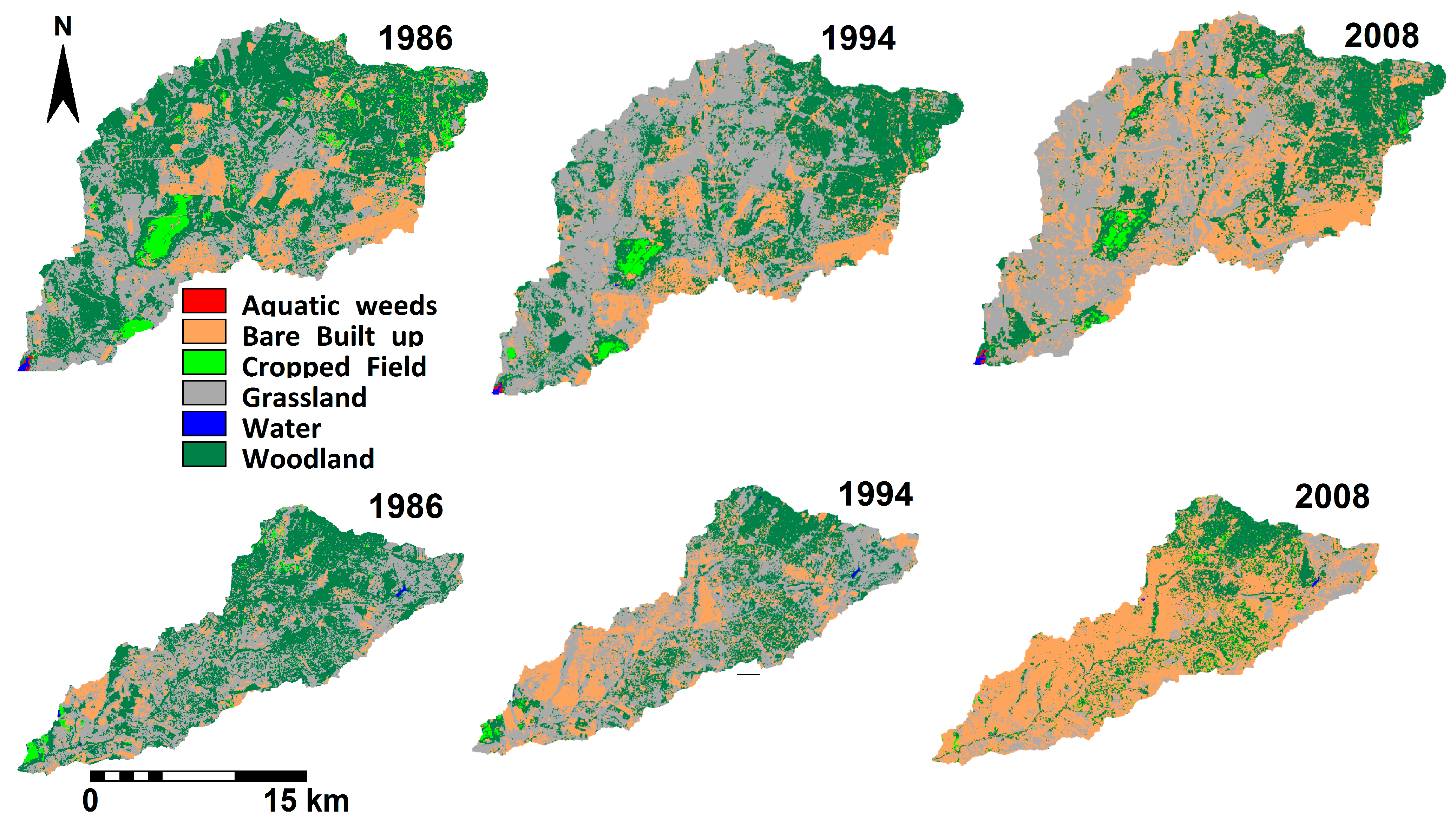
Results of satellite image classification for land cover change assessment in Mukuvisi and Marimba catchments in the city of Harare have shown that the urban area increased by more than 500% in the Mukuvisi catchment and by more than 200% in the Marimba catchment between 1986 and 2008. Woodlands decreased by more than 40% over the same period in the two catchments with a larger decrease in Marimba than in Mukuvisi. Findings on land conversion showed increased conversion of grasslands and woodlands to urban area over the past decades. This accelerated urbanization suggests that several land cover types have been converted to impervious surfaces over the past few decades.

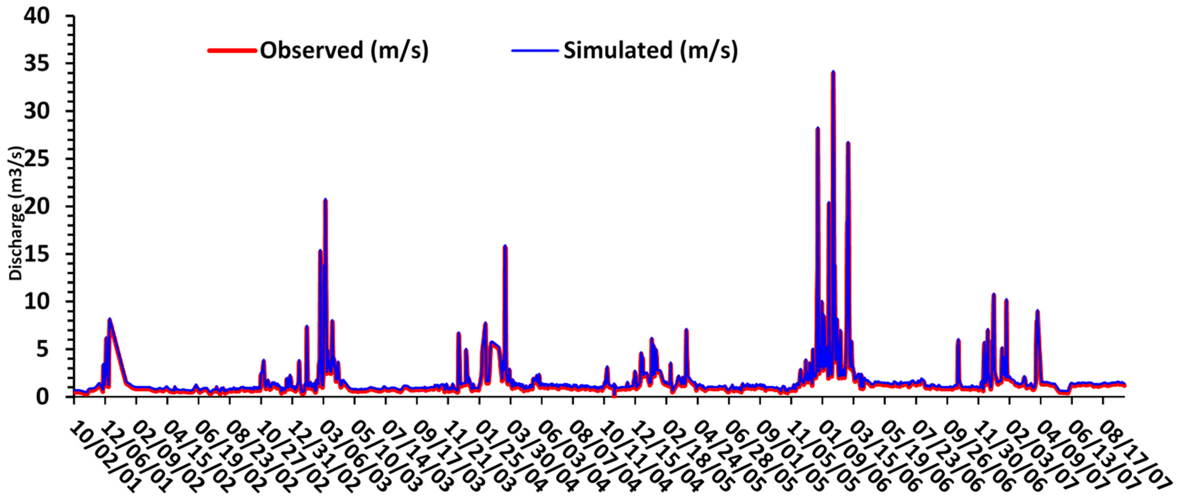
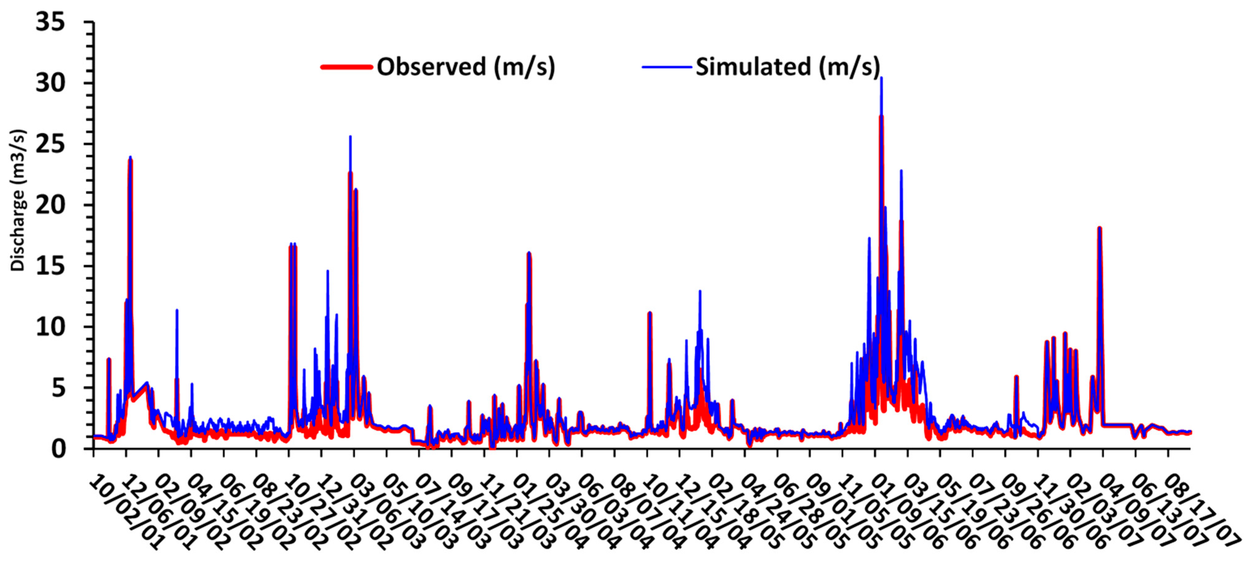
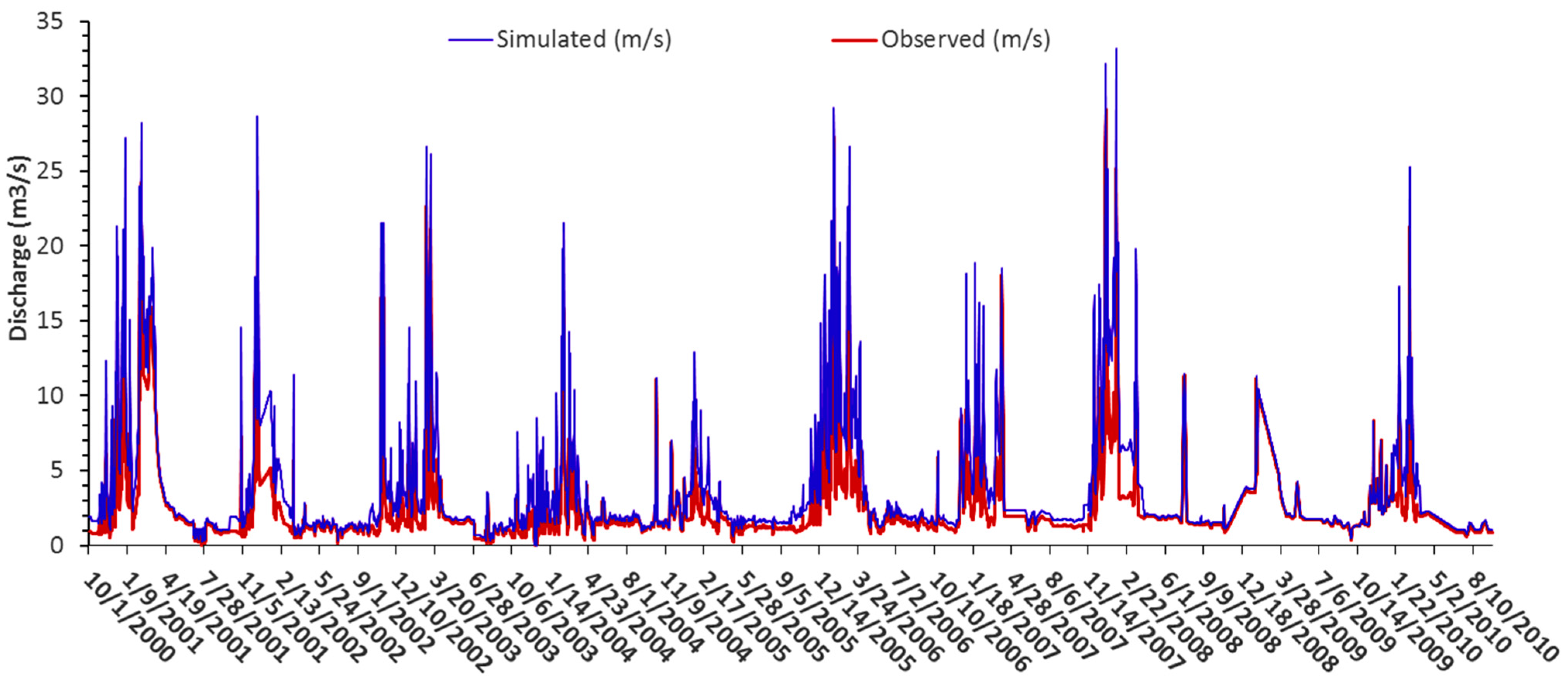
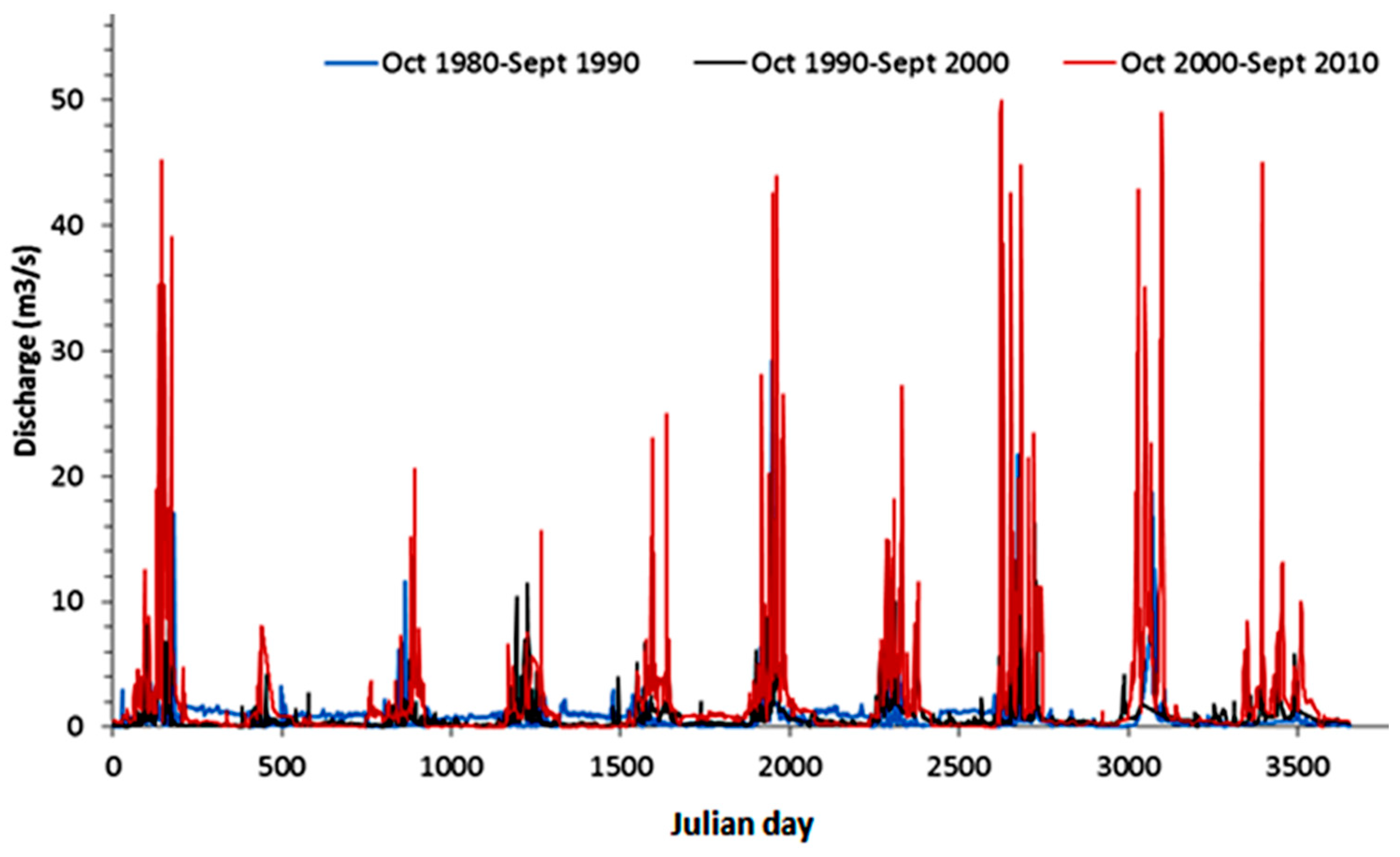
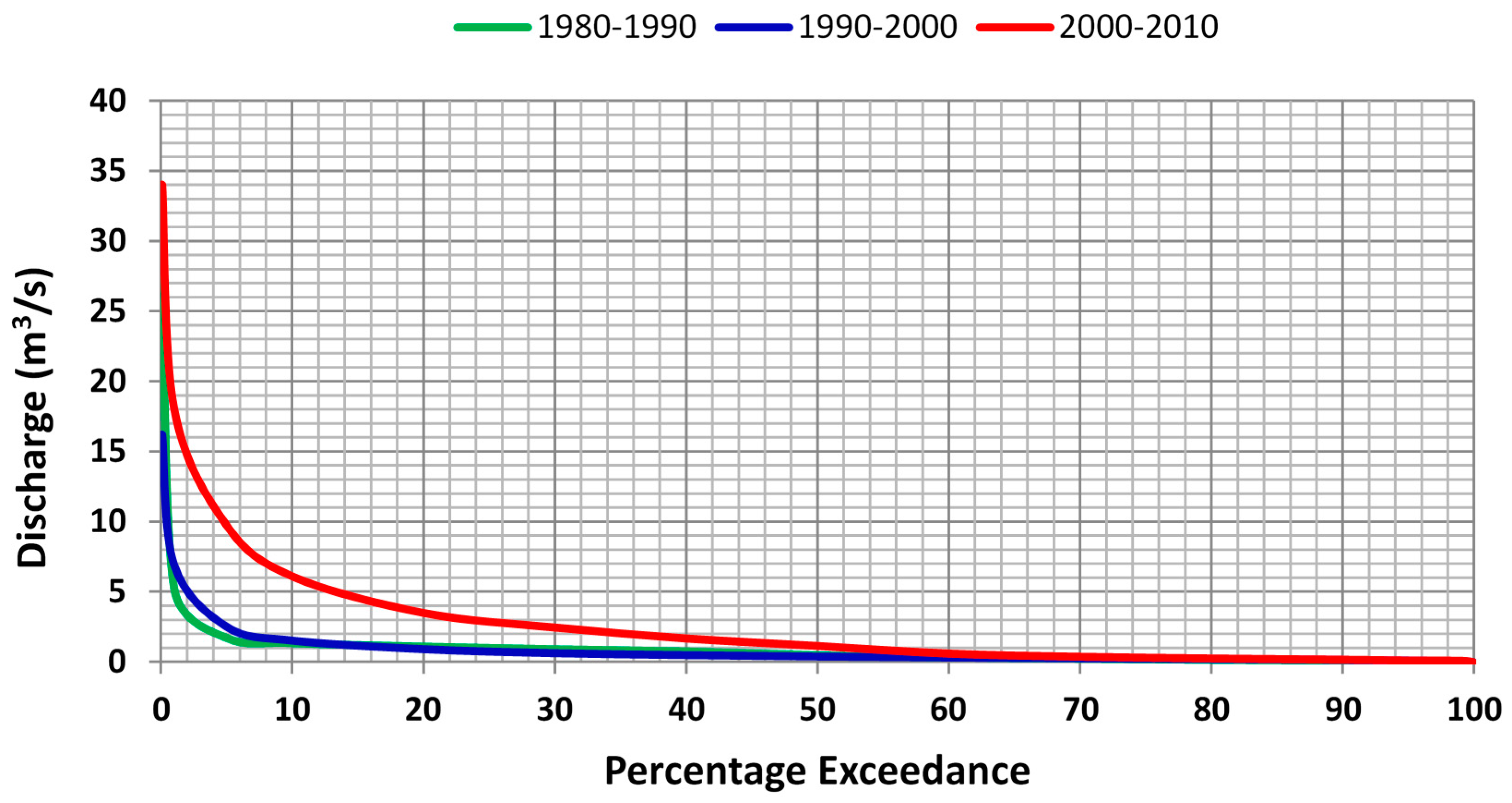
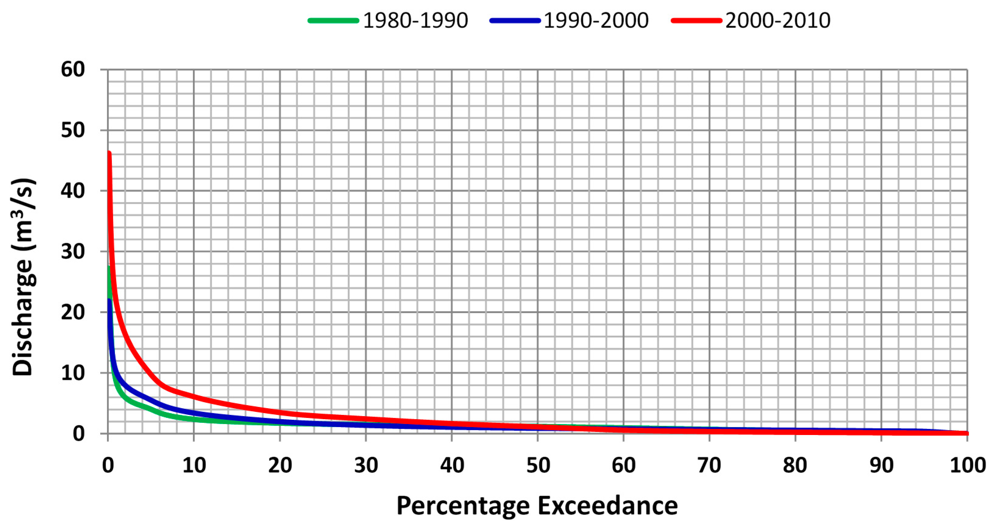
Statistical analysis on rainfall and streamflow time series indicated a significant decreasing trend (p < 0.05) for rainfall and significant increasing trend (p < 0.05) for streamflow. The increasing trends in streamflow could be attributed to the increase in low permeability land surfaces in the two catchments. Results of streamflow modeling for Marimba and Mukuvisi catchments indicated that the mean annual streamflow increased by 46% and 45%, respectively from 1980 to 2010. These increases coincided with the decrease in forest area and an increase in urban area over the same period. As such, findings of this study indicate clear impacts by urbanization in the two catchments. The observed streamflow increases due to land conversions in this study are relatively high compared to other studies (e.g., [82]) which have shown that a 10% increase in imperviousness, results in an increase in the range of 9.8% to 10.2% in annual mean streamflow. A significant impact of urbanization on hydrological regimes is the increase of impervious surfaces, which cause increased streamflow volumes due to the reduction in soil infiltration capacity. As such, urbanized surfaces are likely to generate more runoff than areas, which are densely covered with vegetation especially woodlands. Also, the increase in paved and roofed surfaces reduces the area over which precipitation can infiltrate the soil and results in increased overland flow which, by itself, contributes to quick runoff and streamflow. It can be concluded that clearance of woodlands through urbanization has significantly altered the streamflow regimes in both catchments. These opposing signals in rainfall and streamflow trends signify that the increase in low permeable land surfaces as a result of urbanization probably is the main cause for the streamflow increases.

This study further demonstrated that a widely accepted rainfall-runoff modeling approach can be extended beyond its basic purpose of predicting local variations in water table utilizing the topographic index. To simulate impacts of land use change in this study, land surface parameterization for the rainfall-runoff model was successfully carried out through quantifying the topographic indices, land cover and vegetation indices for urbanization impact assessment. Parameterization served to estimate interception loss, evapotranspiration loss and infiltration excess overland flow by means of the Green and Ampt approach. An approach was applied that used State of the Art GIS and satellite imagery to represent land cover for the years 1986, 1994 and 2008, respectively. For this study, TOPMODEL was run for periods of 10 years which enfolded the dates the satellite images were acquired. This study therefore provided insights into the hydrologic cycle and its regime when a natural or peri-urban catchment undergoes urbanization. Results can be used in the broader spectrum of integrated water resources management and are consistent with observations by [83].

Finally, the study provided insights into hydrologic impacts by an increase in built-up areas and paved surfaces as a result of the urbanization of natural or peri-urban catchments. The findings of this study are highly relevant to many African countries, which are facing accelerated rural-urban migration over the past decades. The latter has been shown in several demographic surveys across Africa with many catchments undergoing rapid urbanization. For instance in Nairobi, Kenya [84] showed the rapid encroachment of urban areas using satellite imagery but hydrological impact assessments are still lacking. Similarly, [85] indicated a rapid increase in urban settlement between 1990 and 2000 in Port Elizabeth, South Africa. These results have important implications on water resources management in Africa, where a number of countries are undergoing rapid urbanization

The authors recommend that besides field measurements to verify model parameters, future work must apply hydrologic models with a clear physical base, such as the Representative Elementary Watershed model (see [86,87]) to allow better evaluation of the impacts of land cover changes and rainfall distributions on the hydrologic regime. In addition, changes in actual evapotranspiration as caused by urbanization must be assessed spatially. Future work also should integrate climate change impacts with impacts of land conversions on streamflow since both have feedback impacts. Therefore, studying these impacts will greatly benefit the water managers in decision-making. In addition, by urbanization, unmonitored wastewater disposal into urban streams have impacts on streamflow and this is scheduled for future work.

References

1. Dube, T.; Gumindoga, W.; Chawira, M. Detection of landcover changes based on traditional remote sensing image classification techniques, around Lake Mutirikwi, Zimbabwe. Afr. J. Aquat. Sci. 2014, 39, 89–95. [Google Scholar] [CrossRef]
2. Wijesekara, G.N.; Gupta, A.; Valeo, C.; Hasbani, J.G.; Qiao, Y.; Delaney, P.; Marceau, D.J. Assessing the impact of future land-use changes on hydrological processes in the Elbow River watershed in southern Alberta, Canada. J. Hydrol. 2012, 412–413, 220–232. [Google Scholar] [CrossRef]
3. Jothityangkoon, C.; Hirunteeyakul, C.; Boonrawd, K.; Sivapalan, M. Assessing the impact of climate and land use changes on extreme floods in a large tropical catchment. J. Hydrol. 2013, 490, 88–105. [Google Scholar] [CrossRef]
4. Meenu, R.; Rehana, S.; Mujumdar, P.P. Assessment of hydrologic impacts of climate change in Tunga-Bhadra river basin, India with HEC-HMS and SDSM. Hydrol. Process. 2013, 27, 1572–1589. [Google Scholar] [CrossRef]
5. Dams, J.; Dujardin, J.; Reggers, R.; Bashir, I.; Canters, F.; Batelaan, O. Mapping impervious surface change from remote sensing for hydrological modeling. J. Hydrol. 2013, 485, 84–95. [Google Scholar] [CrossRef]
6. Furusho, C.; Chancibault, K.; Andrieu, H. Adapting the coupled hydrological model ISBA-TOPMODEL to the long-term hydrological cycles of suburban rivers: Evaluation and sensitivity analysis. J. Hydrol. 2013, 485, 139–147. [Google Scholar] [CrossRef]
7. Ackerman, D.; Stein, E.D. Estimating the variability and confidence of land use and imperviousness relationships at a regional scale1. JAWRA J. Am. Water Resour. Assoc. 2008, 44, 996–1008. [Google Scholar] [CrossRef]
8. Bach, M.; Ostrowski, M. Analysis of intensively used catchments based on integrated modelling. J. Hydrol. 2013, 485, 148–161. [Google Scholar] [CrossRef]
9. Braud, I.; Breil, P.; Thollet, F.; Lagouy, M.; Branger, F.; Jacqueminet, C.; Kermadi, S.; Michel, K. Evidence of the impact of urbanization on the hydrological regime of a medium-sized periurban catchment in France. J. Hydrol. 2013, 485, 5–23. [Google Scholar] [CrossRef] [Green Version]
10. Burns, D.; Vitvar, T.; McDonnell, J.; Hassett, J.; Duncan, J.; Kendall, C. Effects of suburban development on runoff generation in the Croton River basin, New York, USA. J. Hydrol. 2005, 311, 266–281. [Google Scholar] [CrossRef]
11. Rose, S.; Peters, N.E. Effects of urbanization on streamflow in the Atlanta area (Georgia, USA): A comparative hydrological approach. Hydrol. Process. 2001, 15, 1441–1457. [Google Scholar] [CrossRef]
12. Dow, C.L.; DeWalle, D.R. Trends in evaporation and Bowen Ratio on urbanizing watersheds in eastern United States. Water Resour. Res. 2000, 36, 1835–1843. [Google Scholar] [CrossRef]
13. Chu, M.L.; Knouft, J.H.; Ghulam, A.; Guzman, J.A.; Pan, Z. Impacts of urbanization on river flow frequency: A controlled experimental modeling-based evaluation approach. J. Hydrol. 2013, 495, 1–12. [Google Scholar] [CrossRef]
14. Du, J.; Qian, L.; Rui, H.; Zuo, T.; Zheng, D.; Xu, Y.; Xu, C.Y. Assessing the effects of urbanization on annual runoff and flood events using an integrated hydrological modeling system for Qinhuai River basin, China. J. Hydrol. 2012, 464–465, 127–139. [Google Scholar] [CrossRef]
15. Verbeiren, B.; van de Voorde, T.; Canters, F.; Binard, M.; Cornet, Y.; Batelaan, O. Assessing urbanisation effects on rainfall-runoff using a remote sensing supported modelling strategy. Int. J. Appl. Earth Observ. Geoinf. 2013, 21, 92–102. [Google Scholar] [CrossRef]
16. Wang, D.; Gong, J.; Chen, L.; Zhang, L.; Song, Y.; Yue, Y. Spatio-temporal pattern analysis of land use/cover change trajectories in Xihe watershed. Int. J. Appl. Earth Observ. Geoinf. 2012, 14, 12–21. [Google Scholar] [CrossRef]
17. Lillesand, T.M.; Kiefer, R.W. Remote Sensing and Digital Image Interpretation, 4th ed.; Wiley: New York, NY, USA, 2000; p. 724. [Google Scholar]
18. Beven, K. TOPMODEL: A critique. Hydrol. Process. 1997, 11, 1069–1085. [Google Scholar] [CrossRef]
19. Refsgaard, J.C.; Storm, B.; Refsgaard, A. Validation and applicability of distributed hydrological models. In Modelling and Management of Sustainable Basin-Scale Water Resource Systems; IAHS Publ.: Oxfordshire, UK, 1995; No. 231; pp. 387–397. [Google Scholar]
20. Sorooshian, S.; Gupta, V. Model calibration. In Computer Models of Watershed Hydrology; Singh, V.P., Ed.; Water Resources Management Publications: Highlands Ranch, CO, USA, 1995; pp. 23–67. [Google Scholar]
21. Quinn, P.F.; Beven, K.J.; Lamb, R. The Ln(a/TanB) Index: How to calculate it and how to use it within the Topmodel framework. Hydrol. Process. 1995, 9, 161–182. [Google Scholar] [CrossRef]
22. Beven, K.; Freer, J. A dynamic TOPMODEL. Hydrol. Process. 2000, 15, 1993–2011. [Google Scholar] [CrossRef]
23. Beven, K.J. Rainfall-Runoff Modelling: The Primer; John Wiley & Sons: Lancaster, UK, 2001. [Google Scholar]
24. Gumindoga, W.; Rwasoka, D.T.; Murwira, A. Simulation of streamflow using TOPMODEL in the Upper Save River catchment of Zimbabwe. Phys. Chem. Earth. 2011, 36, 806–813. [Google Scholar] [CrossRef]
25. Gunter, A.; Uhlenbrook, S.; Sibert, J.; Leibundgut, C. Multi-criterial validation of TOPMODEL in a mountaneous catchment. Hydrol. Process. 1999, 13, 1603–1620. [Google Scholar] [CrossRef]
26. Huang, B.; Jiang, B. AVTOP: A full integration of TOPMODEL into GIS. Environ. Model. Softw. 2002, 17, 261–268. [Google Scholar] [CrossRef]
27. Nourani, V.; Roughani, A.; Gebremichael, M. TOPMODEL capability for rainfall-runoff modeling of the Ammameh watershed at different time scales using different terrain algorithms. J. Urban Environ. Eng. 2011, 5, 1–14. [Google Scholar] [CrossRef]
28. Braud, I.; Fletcher, T.D.; Andrieu, H. Hydrology of peri-urban catchments: Processes and modelling. J. Hydrol. 2013, 485, 1–4. [Google Scholar] [CrossRef]
29. Valeoa, C.; Moinb, S.M.A. Variable source area modelling in urbanizing watersheds. J. Hydrol. 2000, 228, 68–81. [Google Scholar] [CrossRef]
30. United Nations-Department of Economic and Social Affairs, Population Division. World Population Prospects: The 2012 Revision, Highlights and Advance Tables; Working Paper No. ESA/P/WP.228; United Nations: New York, NY, USA, 2013. [Google Scholar]
31. ZIMSTATS. Census 2012 Preliminary Report; ZIMSTATS: Harare, Zimbabwe, 2012; p. 123. [Google Scholar]
32. Gumbo, B. Re-enginering the urban drainage system for resource recovery and protection of drinking water supplies. In Proceedings of the 2nd WARFSA/WaterNet Symposium: Integrated Water Resources Management: Theory, Practice, Cases, Cape Town, South Africa, 30–31 October 2001.
33. Hranova, R.; Gumbo, B.; Kaseke, E.; Klein, J.; Nhapi, I.; van der Zaag, P. The challenge of integrated water resources management in the Chivero basin, Zimbabwe. In Proceedings of the 2nd WARFSA/WaterNet Symposium: Integrated Water Resources Management: Theory, Practice, Cases, Cape Town, South Africa, 30–31 October 2001.
34. Rwasoka, D.T.; Gumindoga, W.; Gwenzi, J. Estimation of actual evapotranspiration using the Surface Energy Balance System (SEBS) algorithm over land surfaces. J. Phys. Chem. Earth 2011, 36, 736–746. [Google Scholar] [CrossRef]
35. Japanese International Co-Operation Agency (JICA). The Study of Water Pollution Control in Upper Manyame River Basin in the Republic of Zimbabwe; MLGRUD: Harare, Japan; Nippon Jogeduido Sekkei Co. Ltd.: Tokyo, Japan; Nippon Koei Co. Ltd.: Tokyo, Japan, 1996. [Google Scholar]
36. Nhapi, I.; Zvikomborero, Z.; Siebel, M.A.; Gijzen, H.J. Assessment of the major water and nutrient flows in the Chivero catchment area, Zimbabwe. Phys. Chem. Earth 2002, 27, 783–792. [Google Scholar] [CrossRef]
37. Allen, R.G.; Pereira, L.S.; Raes, D.; Smith, M. Crop evapotranspiration-guidelines for computing crop water requirements. In FAO Irrigation and Drainage Paper 56; FAO: Rome, Italy, 1998. [Google Scholar]
38. Tebbs, E.J.; Remedios, J.J.; Harper, D.M. Remote sensing of chlorophyll-a as a measure of cyanobacterial biomass in Lake Bogoria, a hypertrophic, Saline–Alkaline, Flamingo lake, using Landsat ETM+. Remote Sens. Environ. 2013, 135, 92–106. [Google Scholar] [CrossRef]
39. Lu, D.; Weng, Q. A survey of image classification methods and techniques for improving classification performance. Int. J. Remote Sens. 2007, 28, 823–870. [Google Scholar] [CrossRef]
40. Zheng, H.; Zhang, L.; Liu, C.; Shao, Q.; Fukushima, Y. Changes in streamflow regime in headwater catchments of the Yellow River basin since the 1950s. Hydrol. Process. 2007, 21, 886–893. [Google Scholar] [CrossRef]
41. Rientjes, T.H.M.; Haile, A.T.; Kebede, E.; Mannaerts, C.M.M.; Habib, E.; Steenhuis, T.S. Changes in land cover, rainfall and streamflow in Upper Gilgel Abbay catchment, Blue Nile basin—Ethiopia. Hydrol. Earth Syst. Sci. 2011, 15, 1979–1989. [Google Scholar] [CrossRef]
42. Yue, S.; Pilon, P.; Cavadias, G. Power of the Mann-Kendall and Spearman’s rho tests for detecting monotonic trends in hydrological series. J. Hydrol. 2002, 259, 254–271. [Google Scholar] [CrossRef]
43. Kahya, E.; Kalayci, S. Trend analysis of streamflow in Turkey. J. Hydrol. 2004, 289, 128–144. [Google Scholar] [CrossRef]
44. Beven, K.J.; Kirkby, M.J. A physically based, variable contributing area model of basin hydrology. Hydrol. Sci. Bull. Sci. Hydrol. 1979, 24, 43–69. [Google Scholar]
45. Gilbert, R.O. Statistical Methods for Environmental Pollution Monitoring; Wiley: New York, NY, USA, 1987. [Google Scholar]
46. Green, W.H.; Ampt, G. Studies of soil physics, Part I—The flow of air and water through soils. J. Agric. Sci. 1911, 4, 1–24. [Google Scholar] [CrossRef]
47. Barry, D.A.; Parlange, J.Y.; Li, L.; Jeng, D.S.; Crapper, M. Green-Ampt approximations. Adv. Water Resour. 2005, 28, 1003–1009. [Google Scholar] [CrossRef]
48. Swartzendruber, D. Derivation of a two-term infiltration equation from the Green-Ampt model. J. Hydrol. 2000, 236, 247–251. [Google Scholar] [CrossRef]
49. Van den Putte, A.; Govers, G.; Leys, A.; Langhans, C.; Clymans, W.; Diels, J. Estimating the parameters of the Green-Ampt infiltration equation from rainfall simulation data: Why simpler is better. J. Hydrol. 2013, 476, 332–344. [Google Scholar] [CrossRef]
50. Wang, J.; Endreny, T.A.; Hassett, J.M. Power function decay of hydraulic conductivity for a TOPMODEL-based infiltration routine. Hydrol. Process. 2006, 20, 3825–3834. [Google Scholar] [CrossRef]
51. Beven, K.; Lamb, R.; Quinn, P.; Romanowicz, R.; Freer, J. TOPMODEL. In Computer Models of Watershed Hydrology; Sing, V.P., Ed.; Water Resources Publications: Colorado Springs, CO, USA, 1995; pp. 627–668. [Google Scholar]
52. Peters, N.E.; Freer, J.; Beven, K. Modelling hydrologic responses in a small forested catchment (Panola Mountain, Georgia, USA): A comparison of the original and a new dynamic TOPMODEL. Hydrol. Process. 2003, 17, 345–362. [Google Scholar] [CrossRef]
53. Beven, K.J. Infiltration into a class of vertically non-uniform soils. Hydrol. Sci. 1984, 29, 425–434. [Google Scholar] [CrossRef]
54. Wolock, D.M.; McCabe, G.J., Jr. Comparison of single and multiple flow direction algorithms for computing topographic parameters in TOPMODEL. Water Resour. Res. 1995, 31, 1315–1324. [Google Scholar] [CrossRef]
55. Ibbitt, R.; Woods, R. Re-scaling the topographic index to improve the representation of physical processes in catchment models. J. Hydrol. 2004, 293, 205–218. [Google Scholar] [CrossRef]
56. Fedak, R. Effect of Spatial Scale on Hydrologic Modeling in a Headwater Catchment. Master’s Thesis, Virginia Polytechnic Institute and State University, Blacksburg, VA, USA, 1999. [Google Scholar]
57. Gumindoga, W. Hydrologic Impacts of Landuse Change on the Hydrology of Upper Gilgel Abbay Basin—Application of TOPMODEL Concept. Master’s Thesis, University of Twente, Enschede, The Netherlands, 2010; p. 99. [Google Scholar]
58. Ambroise, B.; Beven, K.; Freer, J. Toward a generalization of the TOPMODEL concepts: Topographic indices of hydrological similarity. Water Resour. Res. 1996, 32, 2135–2145. [Google Scholar] [CrossRef]
59. Kim, S.; Delleur, J.W. Sensitivity analysis of extended TOPMODEL for agricultural watersheds equipped with tile drains. Hydrol. Process. 1997, 11, 1243–1261. [Google Scholar] [CrossRef]
60. Kroes, J.G.; van Dam, J.C. Reference Manual SWAP (version 3.0.3); Alterra Green World Research; Alterra-Report 773; Waggeningen UR: Wageningen, The Netherlands, 2003. [Google Scholar]
61. Van Dam, J.C. Field-Scale Water Flow and Solute Transport: SWAP Model Concepts, Parameter Estimation and Case Studies; Wageningen Institute for Environment and Climate Research: Wageningen, The Netherlands, 2000. [Google Scholar]
62. Huete, A.R. A Soil-Adjusted Vegetation Index (SAVI). Remote Sens. Environ. 1988, 25, 295–309. [Google Scholar] [CrossRef]
63. Van Leeuwen, W.J.D.; Huete, A.R.; Walthall, C.L.; Prince, S.D.; Bégué, A.; Roujean, J.L. Deconvolution of remotely sensed spectral mixtures for retrieval of LAI, fAPAR and soil brightness. J. Hydrol. 1997, 188–189, 697–724. [Google Scholar]
64. Parodi, G.N. AHVRR Hydrological Analysis System Algorithms and Theory—Version 1.3. AHAS User Guide; WRES-ITC: Enschede, The Netherlands, 2000. [Google Scholar]
65. Nash, J.E.; Sutcliffe, J.V. River flow forecasting through conceptual models. Part I: A discussion of principles. J. Hydrol. 1970, 10, 282–290. [Google Scholar] [CrossRef]
66. Janssen, P.H.M.; Heuberger, P.S.C. Calibration of process-oriented models. Ecol. Model. 1995, 83, 55–66. [Google Scholar] [CrossRef]
67. De Vos, N.J.; Rientjes, T.H.M. Multi-objective performance comparison of an artificial neural network and a conceptual rainfall-runoff model. Hydrol. Sci. J. 2007, 52, 397–413. [Google Scholar]
68. De Vos, N.J.; Rientjes, T.H.M. Multi-objective training of artificial neural networks for rainfall-runoff modeling. Water Resour. Res. 2008, 44, W08434. [Google Scholar] [CrossRef]
69. Deckers, D.E.H.; Booij, M.; Rientjes, T.M.; Krol, M. Catchment variability and parameter estimation in multi-objective regionalisation of a rainfall-runoff model. Water Resour. Manag. 2010, 24, 3961–3985. [Google Scholar] [CrossRef]
70. Rientjes, T.H.M.; Perera, B.U.J.; Haile, A.T.; Reggiani, P.; Muthuwatta, L.P. Regionalisation for lake level simulation—The case of Lake Tana in the Upper Blue Nile, Ethiopia. Hydrol. Earth Syst. Sci. 2011, 15, 1167–1183. [Google Scholar] [CrossRef]
71. Beven, K.J.; Wood, E.F. Catchment geomorphology and the dynamics of runoff contributing areas. J. Hydrol. 1983, 65, 139–158. [Google Scholar] [CrossRef]
72. Fisher, J.; Beven, K.J. Modelling of streamflow at Slapton Wood using TOPMODEL within an uncertainty estimation framework. Field Stud. 1996, 8, 577–584. [Google Scholar]
73. Lamb, R. Distributed Hydrological Prediction Using Generalised TOPMODEL Concepts. Ph.D. Thesis, Lancaster University, Lancaster, UK, 1996. [Google Scholar]
74. Molicová, H.; Grimaldi, M.; Bonell, M.; Hubert, P. Using TOPMODEL towards identifying and modelling the hydrological patterns within a headwater, humid, tropical catchment. Hydrol. Process. 1997, 11, 1169–1196. [Google Scholar] [CrossRef]
75. Saulnier, G.-M.; Beven, K.; Obled, C. Including spatially variable effective soil depths in TOPMODEL. J. Hydrol. 1997, 202, 158–172. [Google Scholar] [CrossRef]
76. Quinn, P.F.; Beven, K.J. Spatial and temporal predictions of soil moisture dynamics, runoff, variable source areas and evapotranspiration for Plynlimon, Mid-Wales. Hydrol. Process. 1993, 7, 425–448. [Google Scholar] [CrossRef]
77. Doswell, C.A.; Davies-Jones, R.; Keller, D.L. On summary measures of skill in rare event forecasting based on contingency tables. Weather Forecast. 1990, 5, 576–585. [Google Scholar] [CrossRef]
78. Landis, J.R.; Koch, G.G. The measurement of observer agreement for categorical data. Biometrics 1977, 33, 159–74. [Google Scholar] [CrossRef] [PubMed]
79. Wolock, D.M.; Price, C.V. Effects of digital elevation model map scale and data resolution on a topography-based hydrologic model. Water Resour. Res. 1994, 30, 3041–3052. [Google Scholar] [CrossRef]
80. Brown, A.E. Predicting the Effect of Forest Cover Changes on Flow Duration Curves. Ph.D. Thesis, University of Melbourne, Melbourne, VIC, Australia, 2008. [Google Scholar]
81. Kashaigili, J.J.; Majaliwa, A.M. Implications of land use and land cover changes on hydrological regimes of the Malagarasi river, Tanzania. J. Agric. Sci. Appl. 2013, 2, 45–50. [Google Scholar]
82. Bhaduri, B.; Minner, M.; Tatalovich, S.; Harbor, J. Long-term hydrologic impact of urbanization: A tale of two models. J. Water Resour. Plan. Manag. 2001, 127, 13–19. [Google Scholar] [CrossRef]
83. Fohrer, N.; Haverkamp, S.; Eckhardt, K.; Frede, H.G. Hydrologic response to land use changes on the catchment scale. Phys. Chem. Earth Part B Hydrol. Ocean. Atmos. 2001, 26, 577–582. [Google Scholar] [CrossRef]
84. Mundia, C.N.; Aniya, M. Analysis of land use/cover changes and urban expansion of Nairobi city using remote sensing and GIS. Int. J. Remote Sens. 2005, 26, 2831–2849. [Google Scholar] [CrossRef]
85. Odindi, J.; Mhangara, P.; Kakembo, V. Remote sensing land-cover change in Port Elizabeth during South Africa’s democratic transition. South Afr. J. Sci. 2012, 108, 60–66. [Google Scholar]
86. Reggiani, P.; Rientjes, T.H.M. Flux parameterization in the Representative Elementary Watershed (REW) approach: Application to a natural basin. Water Resour. Res. 2005, 41. [Google Scholar] [CrossRef]
87. Reggiani, P.; Rientjes, T.H.M. Closing horizontal groundwater fluxes with pipe network analysis: An application of the REW approach to an aquifer. Environ. Model. Softw. 2010, 25, 1702–1712. [Google Scholar] [CrossRef]