Letter

Evaluation of Radiometric Performance for the Thermal Infrared Sensor Onboard Landsat 8

1
Institute of Remote Sensing and Geographic Information System, Peking University, Beijing 100871, China
2
State Key Laboratory of Remote Sensing Science, School of Geography, Beijing Normal University, Beijing 100875, China
3
Key Laboratory of Agri-Informatics, Ministry of Agriculture/Institute of Agricultural Resources and Regional Planning, Chinese Academy of Agricultural Sciences, Beijing 100081, China
4
ICube Laboratory, Université de Strasbourg, 67412 Illkirch, France
*
Author to whom correspondence should be addressed.
Remote Sens. 2014, 6(12), 12776-12788; https://doi.org/10.3390/rs61212776
Submission received: 11 September 2014 / Revised: 16 November 2014 / Accepted: 15 December 2014 / Published: 19 December 2014
(This article belongs to the Special Issue Recent Advances in Thermal Infrared Remote Sensing)

Abstract

:
The radiometric performance of remotely-sensed images is important for the applications of such data in monitoring land surface, ocean and atmospheric status. One requirement placed on the Thermal Infrared Sensor (TIRS) onboard Landsat 8 was that the noise-equivalent change in temperature (NEΔT) should be ≤0.4 K at 300 K for its two thermal infrared bands. In order to optimize the use of TIRS data, this study investigated the on-orbit NEΔT of the TIRS two bands from a scene-based method using clear-sky images over uniform ground surfaces, including lake, deep ocean, snow, desert and Gobi, as well as dense vegetation. Results showed that the NEΔTs of the two bands were 0.051 and 0.06 K at 300 K, which exceeded the design specification by an order of magnitude. The effect of NEΔT on the land surface temperature (LST) retrieval using a split window algorithm was discussed, and the estimated NEΔT could contribute only 3.5% to the final LST error in theory, whereas the required NEΔT could contribute up to 26.4%. Low NEΔT could improve the application of TIRS images. However, efforts are needed in the future to remove the effects of unwanted stray light that appears in the current TIRS images.

1. Introduction

Landsat 8, prior to launch known as the Landsat Data Continuity Mission (LDCM), launched on 11 February 2013, is the latest in the series of Landsats. The payload of Landsat 8 consists of two push-broom instruments, namely, the Operational Land Imager (OLI, nine bands in visible, near-infrared, and shortwave infrared wavelengths) and Thermal Infrared Sensor (TIRS, two bands, 10 (10.6 µm–11.19 µm) and 11 (11.5 µm–12.51 µm)). These two instruments provide a global coverage every 16 days with a field-of-view (FOV) of approximately 15° at spatial resolutions of 30 m (OLI) and 100 m (TIRS). Unlike previous Landsat satellites (4, 5 and 7), which have only one thermal infrared band, the TIRS instrument pioneers a new technology, namely quantum well infrared photodetectors, to measure the thermal radiation of the Earth in two bands [1,2,3]. Theoretically, a split window (SW) algorithm, instead of a single-channel method [4,5], can be proposed for the two thermal bands to retrieve global land surface temperature (LST) with high accuracy [6,7].
TIRS was calibrated before its launch, but its radiometric performance may be affected by any potential changes in the optical status of the instrument generated in the rapid launch process and the long period of post-launch in the orbit. To optimize the use of TIRS data, knowledge about the noise in TIRS images is important before their quantitative applications in retrieving LST, sea surface temperature and atmospheric water vapor [2,5,8]. Noise is considered as the random error that will contaminate the signal (i.e., the useful information) and affect image quality, stability and uniformity. For thermal infrared data, noise-equivalent change in temperature (NEΔT) is most often used to investigate image noise level. The TIRS noise requirements were specified in terms of noise-equivalent change in radiance (NEΔL) and were ≤0.059 W/(m2∙μm∙sr) for Band 10 and ≤0.049 W/(m2∙μm∙sr)) for Band 11. This corresponded to NEΔTs of 0.80 K at 240 K, 0.4 K at 300 K and 0.27 K at 360 K for Band 10 and 0.71 K at 240 K, 0.4 K at 300 K and 0.29 K at 360 K for Band 11 [1]. However, these NEΔTs are larger than those of similar thermal infrared bands of the Moderate Resolution Imaging Spectroradiometer (MODIS, 0.05 K) [9,10] and Advanced Very High Resolution Radiometer (AVHRR, 0.1 K) [11]. They could, therefore, cause significant uncertainty in LST retrieval. To characterize the radiometric performance for possible post-launch degradation, the radiometric characteristics of the TIRS instrument are assessed in the orbit by observing deep space and the onboard blackbody calibrator [1]. This enables monitoring of the stability and noise of each single detector.
In order to optimize the use of TIRS images, this study estimates the radiometric noise (i.e., NEΔT) of TIRS bands from resampled georeferenced observed images of different uniform land covers, such as lake, deep oceans, snow, desert and Gobi, as well as densely-vegetated surface. Consequently, it is organized as follows: Section 2 will introduce the method and the data used to estimate temperature noise, and Section 3 will present temperature noise and its variation with brightness temperature and the NEΔT of TIRS bands. Section 4 and Section 5 will conduct discussion and conclusions, as well as prospective future work.

2. Method and Data

2.1. Method

To estimate the NEΔT for the TIRS two bands, finding some ground sites where the surface and atmospheric conditions are uniform is crucial. In such uniform sites, the pixel brightness temperature can be expressed as follows [9,12]:
T b ( c , j ) = T b , s u r f ( c ) + δ T b , n o i s e ( c , j ) + δ T b , s a ( c , j )
where b = 1 to 2 and stands for the TIRS band number. c is the detector number, because TIRS observes a surface with a push-broom manner by using a linear detector array for each band, which is different from the Thematic Mapper (TM) and Enhanced TM Plus (ETM+), with a whisk-broom manner. If the radiometric response is not the same for all detectors, the brightness temperature will change pixel by pixel. j is the pixel number over the study area. Tb,surf(c) is the brightness temperature at average surface and atmospheric conditions if no noise and change exist in surface and atmosphere conditions in the study area. δTb,noise(c, j) is the contribution to the brightness temperature due to the noise of the detector. δTb,s−a(c, j) is the effect of the variations in surface and atmospheric conditions. For a uniform area, if no variation exists in surface and atmospheric conditions, i.e., δTb,s−a(c, j) = 0, and all detectors of each band are assumed to have the same radiometric characteristics, then Equation (1) will change to:
T b ( j ) = T b , s u r f + δ T b , n o i s e ( j )
In Equation (2), the exact noise δTb,noise(j) for each pixel is difficult to determine. However, the temperature noise level may be evaluated by using the standard deviation σ of the pixel brightness temperature in the uniform area, i.e.,
T b , s u r f = 1 n i = 1 n T b ( j )
σ = δ T b , n o i s e = 1 n 1 i = 1 n [ T b ( j ) T b , s u r f ] 2
where n is the number of pixels in the uniform area. The average of the temperature noise σ at different times and places can be finally considered as an estimate of NEΔT at given temperatures. For clarity, the term temperature noise (or noise) in the following discussion mainly means the variation of pixels’ brightness temperatures in the uniform area and land covers, while the term NEΔT corresponds to the general assessment of the temperature noise level for the instrument’s band. Besides, note that, because all detectors of each band were assumed to have the same radiometric characteristics, the estimated NEΔT based on Equation (4) is the average noise level for all detectors, rather than each single detector.
The abovementioned method of estimating NEΔT is generally operational, because it only needs to find uniform surfaces, which can be achieved in large lake, deep ocean, snow, desert and dense vegetation. However, an absolutely “uniform” surface is impossible to find in a large area in satellite images, and variations of surface and atmospheric conditions between pixels in the selected area are inevitable. Consequently, the NEΔT in Equation (4) will be slightly overestimated.

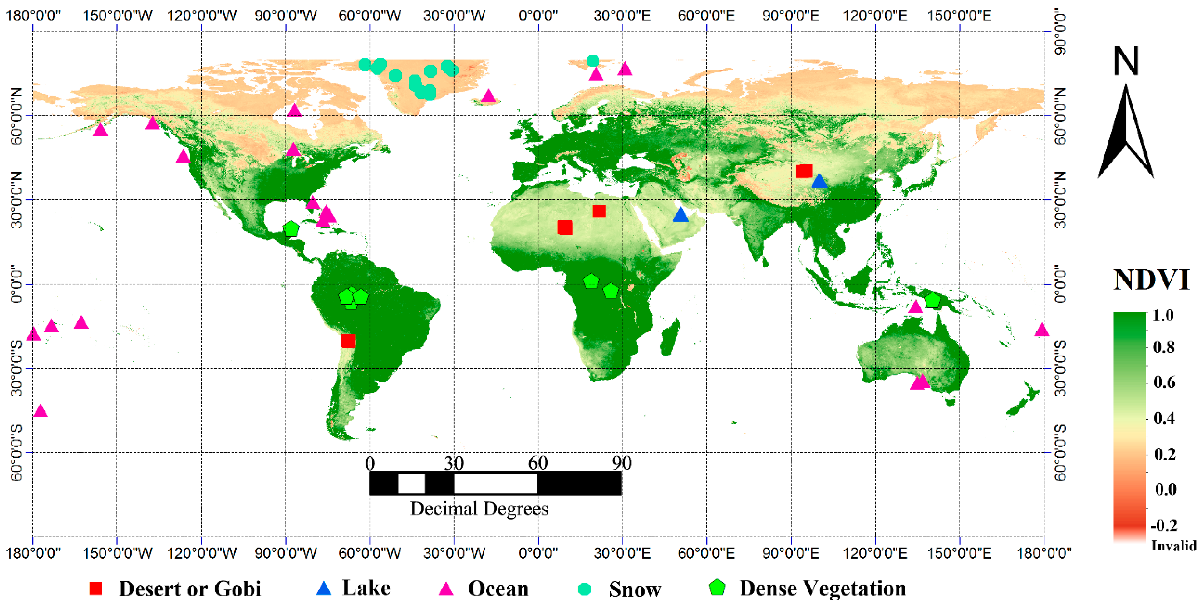
2.2. Landsat 8 Image Data

Large lakes and oceans are good candidates for uniform areas, because the surface temperature in the center of lakes or in the oceans far from land shows small variation. Given that the noise requirements are fixed values of NEΔL, the NEΔT of TIRS bands may decrease with brightness temperature [1]. Therefore, TIRS images at different brightness temperatures must be selected. Some additional land covers, including desert or Gobi, snow and dense vegetation, were also selected in this study, because these land covers can be distributed uniformly in a large area in satellite images. In the selected land covers, snow is expected to provide a low value of brightness temperature, whereas desert may present a high value of brightness temperature.
Finally, we chose a total of 45 ground sites, as shown in Figure 1, including 2 lake sites, 20 deep ocean sites, 13 snow sites, 4 desert or Gobi sites and 8 dense vegetation sites. We downloaded a total of 339 images before the end of May 2014, under clear sky conditions from the U.S. Geological Survey (USGS) website [13]. The background image of Figure 1 was driven from the MODIS global Normalized Difference Vegetation Index (NDVI) product at a spatial resolution of 0.05°. Among the sites, Qinghai Lake (Lon = 100.0°E, Lat = 36.8°N) in China, which was often used for satellite calibrations [14], and the Gulf of Bahrayn (Lon = 50.8°E, Lat = 24.9°N) were chosen. Four desert or Gobi sites (see red squares), including Dunhuang Gobi calibration sites (Lon = 94.0°E, Lat = 40.1°N) in China [15], a Sahara desert site in Niger (Lon = 9.0°E, Lat = 20.2°N) and the Uyuni Salt Flat in Bolivia (Lon = −68.0°W, Lat = −20.0°S) were chosen from the USGS Radiometry Test Site Gallery [16] because of their flat and uniform surfaces in large areas. The snow sites were close to the North Polar Region, and the dense vegetation was mainly distributed in the Amazon region and southern Africa. Given that we had no access as a public user to download ocean images from the USGS website, the ocean near some small islands was used for investigation.
Uniform sub-areas around the ground sites in the images were manually selected. On the one hand, the size of such sub-areas cannot be small, because this will reduce the representativeness of the obtained result. On the other hand, the size cannot be large, because the variations in surface and atmospheric conditions intensify as the size increases. After trial and error, we found that an area of about 1 km × 1 km (about 33 samples × 33 lines of pixels; note that the TIRS image downloaded from the USGS website was actually resampled from 100 m to 30 m for combined use with OLI images) is reasonable, and a meaningful result can be obtained for the temperature noise from Equation (4). Furthermore, the NDVI, Normalized Difference Water Index (NDWI) [17], Normalized Difference Snow Index (NDSI) [18] and Normalized Difference Building-up Index (NDBI) [19] of each pixel in the sub-areas were estimated from OLI reflectance at the top of the atmosphere. To ensure uniform sub-areas, with dense vegetation as an example, pixels with NDVI out of the range ( x ¯ 2 δ ,   x ¯ + 2 δ ) (where x ¯ is the average of the NDVI and δ is the standard deviation of NDVI) were removed before noise calculation. If the removed pixels covered more than 5% of the pixel number of one sub-area, the sub-area was consequently abandoned. Similarly, the same threshold method was applied to check the surface condition variation of lake and deep ocean from NDWI, snow from NDSI and desert and Gobi from DNBI.
Figure 1. Distributions of the ground sites. The background image came from the MODIS global NDVI product at Day 257, 2013, with a spatial resolution of 0.05°.
Remotesensing 06 12776 g001

3. Results and Analysis

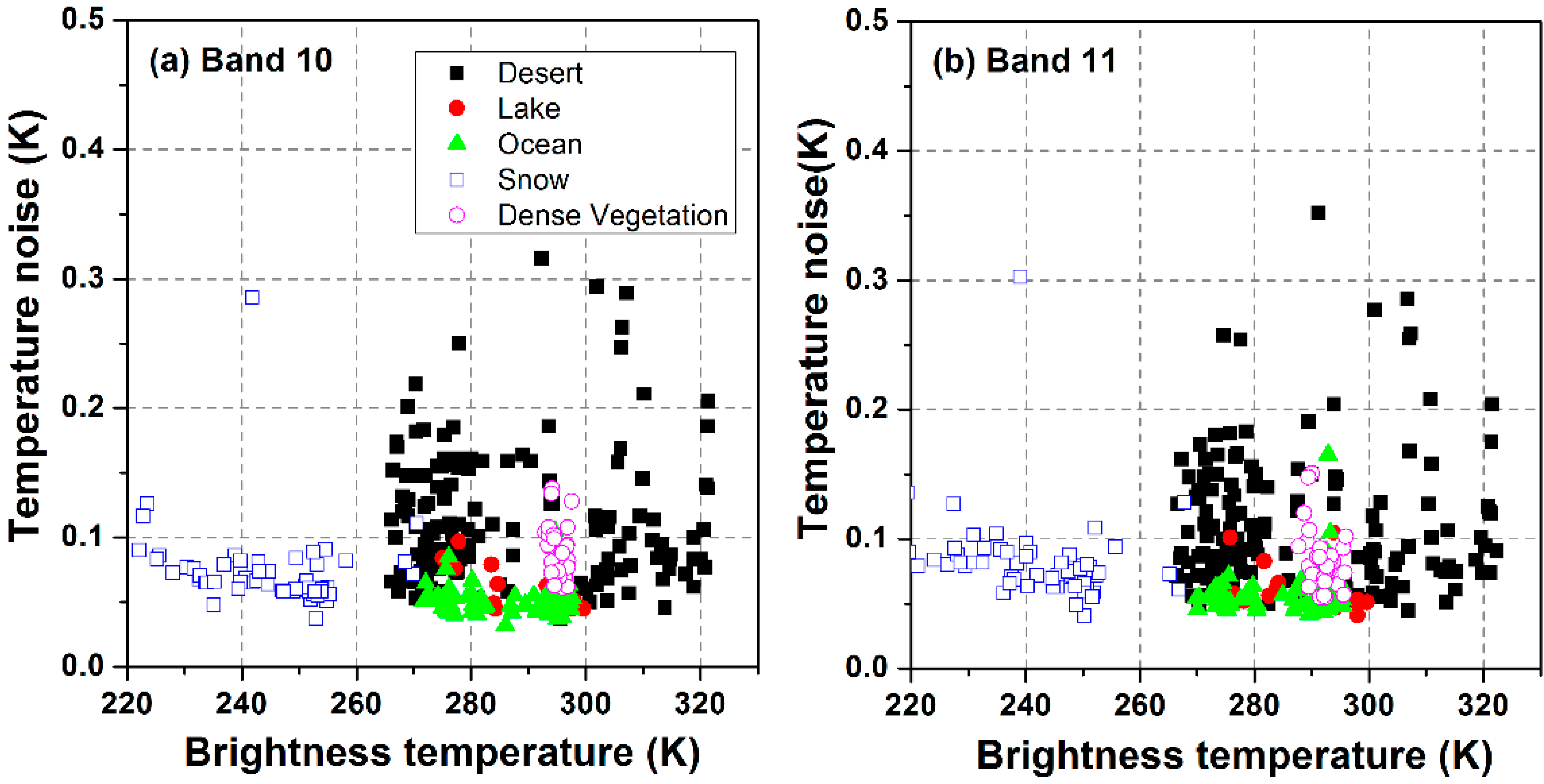
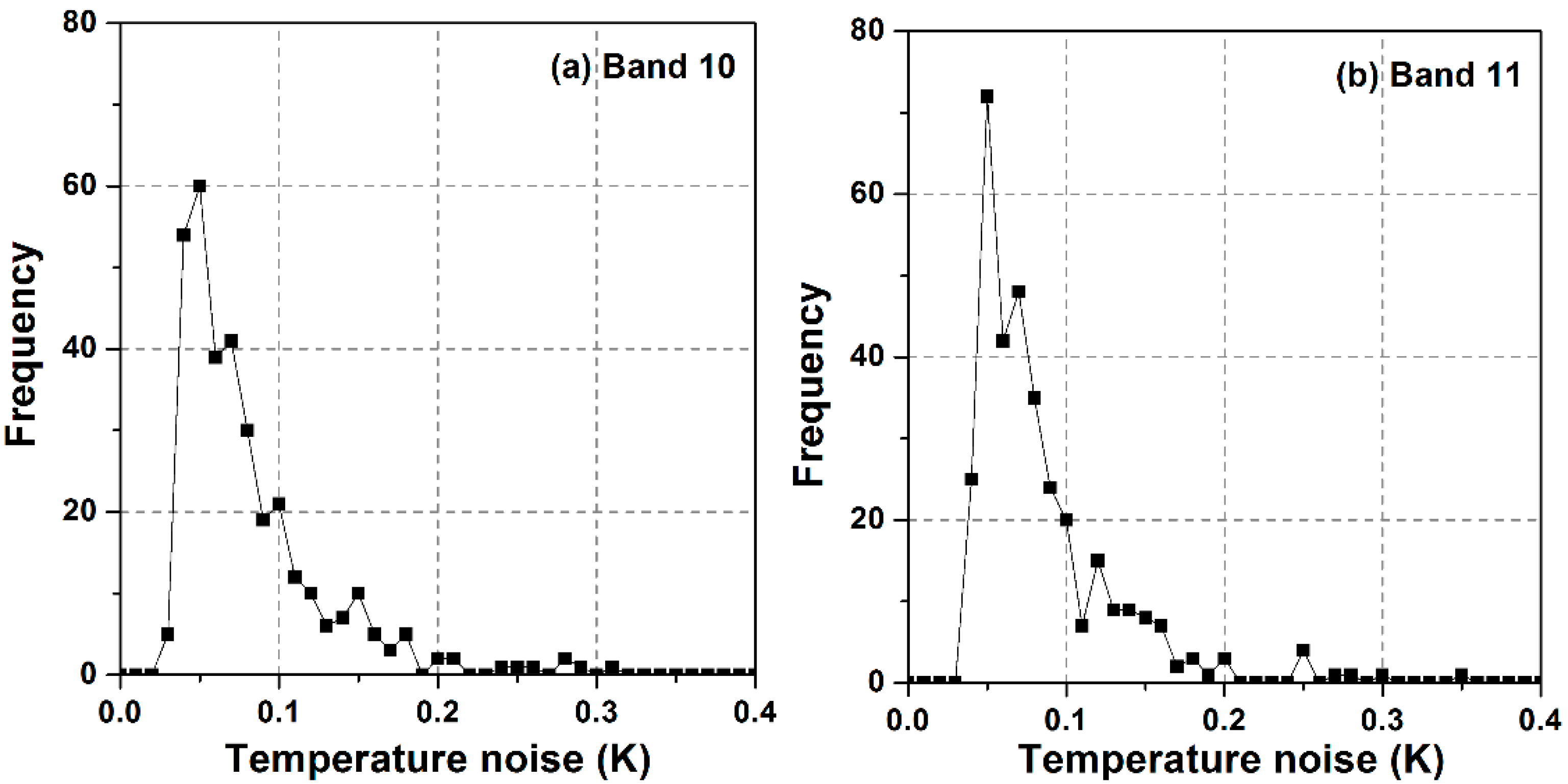
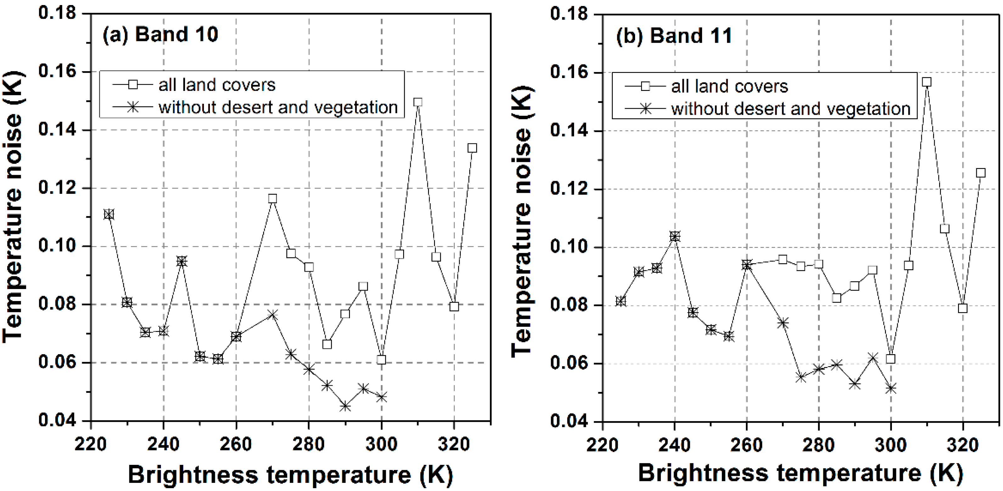
3.1. NEΔT of TIRS Images

To calculate NEΔT, the brightness temperature from the measured digital number (DN) must be obtained as follows:
L λ = a λ × D N + b λ ,   T = k 2 ln ( k 1 / L λ + 1 )
where aλ and bλ are the radiometric calibration rescaling coefficients and k1 and k2 are the channel-dependent coefficients used to transfer apparent radiance to brightness temperature T (K). All of the coefficients can be found in an auxiliary file along with the images [20]. Using Equations (3)–(5), we obtained the ranges of brightness temperature (BT) and temperature noise for different land covers, as listed in Table 1. The brightness temperature approximately ranged from 218 K (low temperature from snow) to 322 K (high temperature from desert). The temperature difference of each land cover was up to tens of Kelvins, because its images came from different places at different dates. Table 1 also shows that the temperature noise mainly ranged from 0.05 K to 0.35 K, but depended on the land covers.
To elucidate the temperature noise, we present σ (see Equation (4)) of all of the selected uniform sub-areas in the ground sites (see Figure 2). The temperature noise of the two bands fell within 0.1 K for most cases of snow, lake, deep ocean and dense vegetation, but was larger than 0.1 K and close to 0.4 K (the designed requirement) for some desert/Gobi samples (see black square). Such large noises for desert were probably caused by the inner variation of the desert surface composed of different materials with different reflectances and emissivities. A comparison between Figure 2a,b showed that the noise of Band 10 was smaller than that of Band 11, especially for the low (snow) and high brightness temperatures (desert). However, their difference was not significant.
Table 1. Ranges of brightness temperature and its temperature noise σ for different land covers. The terms Max, Min and Avg. correspond to the maximum, minimum and average values, respectively.
Band 10
Land CoversMin BT (K)Max BT (K)Avg. σ (K)Min σ (K)Max σ (K)
Lake275.0299.60.0590.0450.097
Ocean271.8297.60.0510.0320.105
Snow222.1270.50.0730.0410.286
Desert266.1321.30.1120.0370.316
Dense vegetation292.9297.50.1010.0610.138
Band 11
Lake275.8299.60.0620.0410.105
Ocean269.8295.50.0570.0420.165
Snow217.9267.70.0840.0410.303
Desert266.3322.30.1120.0450.352
Dense vegetation287.3296.00.1100.0550.151
Figure 2. Temperature noise of the TIRS two bands for different land covers and brightness temperatures.
Remotesensing 06 12776 g002
Figure 3 shows the temperature noise histograms of the TIRS two bands in an interval of 0.01 K. Approximately 72.8% and 72.1% points with noise less than 0. 1 K existed for Bands 10 and 11, respectively. Only a few points (approximately 2%) had a value larger than 0.25 K. These results indicated that the temperature noise included in the two bands was generally small.
Figure 3. Histograms of temperature noise for the TIRS two bands based on the ground samples.
Remotesensing 06 12776 g003
Figure 4. Variation of temperature noise with brightness temperature for the TIRS two bands. Unfilled squares stand for the noise calculated from all land covers, while the stars stand for the result calculated without desert and vegetation samples.
Remotesensing 06 12776 g004
To investigate the variation of noise with the brightness temperature, the brightness temperature ranges (approximately from 218 K to 322 K, as shown in Figure 2) of the two bands were divided into several subranges with a step of 5 K. Consequently, the average temperature noise of each subrange was calculated, as presented in Figure 4 (see the unfilled squares). In this figure, the temperature noise of most temperature subranges was smaller than 0.1 K, and its variation with the brightness temperature was not as strong as that of the designed specifications, though it had a relatively large fluctuation in the brightness temperature range of 295 K to 325 K. In Figure 2, this temperature range was mainly for the desert/Gobi and vegetation surface. The large noise in this range was probably caused by the variations of surface and atmospheric conditions, rather than the intrinsic feature of the thermal infrared bands. From this point of view, the desert and vegetation samples were possibly not suitable for the evaluation of the temperature noise, because of its “strong” non-uniformity. In order to reduce this influence, we recalculated the noise for each temperature subrange without desert and vegetation samples and showed the new results in Figure 4 (see the stars). A comparison indicated that the temperature noise of the lake, deep ocean and snow samples was significantly smaller than that calculated from all land covers in the temperature range of 275 K to 300 K. Because, as shown in Table 1, the brightness temperature of lake, deep ocean and snow samples was smaller than 300 K and it is difficult to find those covers with a brightness temperature larger than 300 K, the noise for larger temperature cannot be estimated. However, as shown Figure 4, the new estimated noise was found to generally decrease with the increase of the brightness temperature [1,21], and consequently, it is reasonable to think that the noise is around 0.05 K~0.06 K for temperatures larger than 300 K.
Based on the results in Figure 2, Figure 3 and Figure 4, the NEΔT was calculated as the average value of the noise in the specified temperature range. For comparison with the design required value, we used the average noise value in the temperature range from 230 K to 250 K as the NEΔT at 240 K, the average noise value of 270 K to 290 K as the NEΔT at 280 K and the average noise value of 290 K to 310 K as the NEΔT at 300 K. As a result, the NEΔT at different brightness temperatures for the two bands are listed in Table 2. Columns 2–4 showed the results calculated from all land cover samples, while the last three columns were the results without desert and vegetation samples. From Table 2, we knew that the potential surface non-uniformity of desert and vegetation impacted the NEΔT remarkably and almost increased by 50% compared to the NEΔT calculated only from lake, deep ocean and snow samples. Since lake, deep ocean and snowy regions were usually more uniform, the NEΔT based on those land covers should be more reliable. Therefore, the values in the last three columns of Table 2 were finally considered as the estimated NEΔT of the TIRS two bands. Those levels of NEΔT were close to that of MODIS and AVHRR, better than the design specification (e.g., 0.71 K at 240 K and 0.4 K at 300 K) [1], TM (0.17–0.30 K at 280 K) and ETM+ (0.22 K at 280 K for high gain observation and 0.28 K for low gain observation) [22]. According to the work of the Landsat Calibration/Validation team [23], the observed NEΔT of this study is very close to the average values of NEΔT (0.048 K for Band 10, and 0.052 K for Band 11) derived from the onboard blackbody source, especially at 280 K and 300 K (Table 2). This small difference indicated that our scene-based method from uniform ground sites is feasible to evaluate NEΔT, and it can be regarded as a vicarious method if the onboard calibration source does not work well enough, because of the aging and degradation of instruments and other reasons.
Table 2. NEΔT of the TIRS two bands at different brightness temperatures.
Band No.From All Land CoversWithout Desert and Vegetation
240 K280 K300 K240 K280 K300 K
Band 100.0750.0890.0860.0750.0550.051
Band 110.0830.0910.0920.0830.0560.060
However, as stated above, an important assumption used to evaluate temperature noise was that the surface and atmospheric conditions were as uniform as possible. Although we selected homogenous sub-areas carefully and used some spectral indices (NDVI, NDWI, NDSI and NDBI) to remove some invalid pixels, the changes of surface and atmospheric conditions (even for lake, deep ocean and snow) were inevitable. As a result, the standard deviation in Equation (4) was actually contributed by the real temperature noise involved in the images and the error from surface and atmospheric variations. Considering that the surface and atmospheric variations are impossible to remove completely, NE∆T was overestimated in theory. This might be the reason that caused NEΔT at 300 K for Band 10 to be slightly larger than that at 280 K, as shown in Columns 6 and 7 of Table 2.

3.2. Effect of NEΔT on LST Retrieval

The SW algorithm can be applied to retrieve LST from the TIRS two band images, and several studies have addressed this issue [6,7]. We also developed an operational SW algorithm [24] for TIRS data. In our algorithm, LST was retrieved from a nonlinear combination of the brightness temperatures of two bands, i.e., LST = A0 + A1·T10 + A2·T11 + A3·(T10T11)2, where the coefficient Ai (i = 0, 1, 2, 3) was determined from simulated data under different atmospheric and surface conditions and depended on atmospheric water vapor content ranges. The SW algorithm can cause an error of about 0.34 K for the retrieved LST for the typical water vapor range [0.0, 2.5] g/cm2 if no noise were contained in the input brightness temperatures and other parameters. To analyze the influence of NEΔT on LST retrieval, we added a Gaussian-distributed noise with a zero mean and a standard deviation equal to 2 × NE∆T (at 300 K) to the input brightness temperatures (Ti and Tj) of the two bands of TIRS, and finally, the LST error from the above SW algorithm became 0.352 K for water vapor within [0.0, 2.5] g/cm2. Compared to the LST error (0.34 K) caused by the conditions with noise-free brightness temperatures, the NE∆T obtained in this study only caused an error of approximately 0.012 K to the LST, which contributed approximately 3.5% to the total LST error (0.352 K). However, if the designed NEΔT (approximately 0.4 K) was used, the total LST error changed to 0.462 K, in which the designed NEΔT contributed about 0.122 K (covering 26.4%). Therefore, the NEΔT evaluation in this study is crucial for us to determine the exact noise level for TIRS images and its effect on LST retrieval and other applications. However, note that we here only investigated the effect of NEΔT on the LST retrieval from the theoretical SW algorithm, and more considerations, such as the unwanted stray light (see Figure 5 in Section 4.2 and [25]) in the current TIRS images and the uncertainty included in atmospheric data and emissivity, should be concerned in the practical applications of the SW algorithm.
Figure 5. An example of TIRS images with spatial discontinuity. (a) False-color image from Operational Land Imager (OLI) near-infrared, red and green bands; (b) Band 10 of TIRS; (c) Band 11 of TIRS.
Remotesensing 06 12776 g005

4. Discussions

In the above discussion, the NEΔT of the TIRS two bands was obtained with several important assumptions and simplifications, which were reasonable for most cases with uniform surfaces. However, to monitor the noise level of TIRS images in a long period completely, two important aspects have to be addressed in the future.

4.1. Time Variation of the Radiometric Response of the Instrument

TIRS instrument was designed to provide thermal multispectral image data of no less than three years. Given that the response of the instrument to the input energy may vary over time, the absolute radiometric calibration coefficients and noise level (NEΔT) should be updated as necessary [2,26]. This is currently in the plan for TIRS and ground measurements, such as those described here, provided a valuable check on the onboard calibration system. However, this study actually ignored the possible time variation of radiometric calibration coefficients and temperature noise. This condition is reasonable at the beginning of the TIRS mission, but considerable attention should be paid to such time variation in the future, especially at the end of the mission, when the instrument will probably show uncertainty and instability.

4.2. Pixel-to-Pixel Radiometric Variation in the Linear Array System

According to Equations (3) and (4), this study used the spatial standard deviation in uniform surfaces to calculate the noise level with an important assumption that all TIRS detectors of one band have the same radiometric characteristics. As reported recently [25], although the radiometric characteristics exist among the different detectors, for a 300-K blackbody, the observed maximum variation of an individual detector from the band average response is approximately 0.05% in Band 10 and 0.2% in Band 11. However, after checking hundreds of TIRS images in different places, we found that TIRS images suffer from the problem of spatial discontinuity in some places. Figure 5 shows an example of TIRS images with this problem: there was no obvious strip in Figure 5a (the false-color image composed of OLI near-infrared (Band 5: 0.845–0.885 μm), red (Band 4: 0.630–0.680 μm) and green bands (Band 3: 0.525–0.600 μm)), while some strips were found in both Figure 5b,c (TIRS two bands). This region (center Lon = −66.08°W, Lat = −5.83°S, path = 1, row = 64; date: 26 September 2013) is located in the Amazon rainforest of southern Africa. As we know, the linear array detectors of the TIRS two bands are composed of three modules in the focal plane [1]; however, stray light (i.e., signals from outside the FOV (about 15°)) was recently found to enter the optical system and to add to the direct line-of-sight signal recorded by the focal plane arrays, and consequently, some overlapping regions become visible between two adjacent focal plane modules [25]. The Landsat calibration term is trying to find an effective way to remove such stray light from the useful signals, and the TIRS performance is expected to improve after the correction for stray light is implemented. Unfortunately, we also had no method to correct this non-uniformity in this study, and actually had tried to avoid selecting surface samples in the overlapping area to make our results applicable for most detectors.

5. Conclusions

The radiometric noise of the remotely-sensed image is a key parameter to assess the uncertainty involved in the applications of this image. This study evaluated the noise level of the TIRS two thermal infrared bands from a scene-based method by using clear-sky images at 45 uniform ground sites, including lake, deep ocean, snow, desert and Gobi, as well as dense vegetation areas. Results revealed that the temperature noise decreased with the increasing brightness temperature in the range of 220 K to 300 K, and the estimated NEΔT was, respectively, 0.075 K at 240 K, 0.055 K at 280 K and 0.051 K at 300 K for TIRS Band 10 and was, respectively, 0.083 K at 240 K, 0.056 K at 280 K and 0.060 K at 300 K for TIRS Band 11. Those observed NEΔTs were smaller than the design requirement NEΔT (e.g., 0.4 K at 300 K) and close to the average NEΔT (0.048 K for Band 10, and 0.052 K for Band 11) estimated from the onboard blackbody source, which meant that this scene-based method from uniform ground sites is feasible to evaluate NEΔT, especially for the conditions that the onboard blackbody does not work well enough. We also analyzed the effect of NEΔT on LST retrieval from our newly-developed SW algorithm and found that the new observed NEΔT contributed only 3.5% to the LST error, whereas the design-specified NEΔT (0.4 K) contributed approximately 26.4% to the LST error in theory. Therefore, the small NEΔT of TIRS is expected to improve future applications of TIRS images in retrieving land surface and other parameters. However, considering the aging of detectors, future work should pay considerable attention to the time variation of the noise, and efforts are also needed to remove the unwanted stray light that comes from outside the TIRS FOV and appears in the current images to improve the data quality of TIRS images.

Acknowledgments

The authors would like to thank the four anonymous reviewers for their constructive and thoughtful comments and suggestions, and they also thank the USGS for downloading freely Landsat 8 images from their data archive. This work was supported by the program of the National Natural Science Foundation of China (Grant Nos. 41401375, 41230747, 41331171, 41231170 and 41471430), the China Post-doctoral Fund (Grant No. 2014M550551), the National Basic Research Program of China (Grant No. 2013CB733402) and the High Resolution Earth Observation Systems of National Science and Technology Major Projects.

Author Contributions

In this manuscript, Huazhong Ren provided the main ideas, evaluated the radiometric performance and also wrote the whole manuscript. Chen Du, Rongyuan Liu and Qiming Qin evaluated the radiometric performance and helped much with processing of Landsat 8 data. Jinjie Meng contributed by generating some of the graphs, and Zhao-Liang Li and Guangjian Yan made many revisions to the whole manuscript.

Conflicts of Interest

The authors declare no conflict of interest.

References

  1. Irons, J.R.; Dwyer, J.L.; Barsi, J.A. The next Landsat satellite: The Landsat Data Continuity Mission. Remote Sens. Environ. 2012, 122, 11–21. [Google Scholar] [CrossRef]
  2. Roy, D.P.; Wulder, M.A.; Loveland, T.R.; Woodcock, C.E.; Allen, R.G.; Anderson, M.C.; Helder, D.; Irons, J.R.; Johnson, D.M.; Kennedy, R.; et al. Landsat-8: Science and product vision for terrestrial global change research. Remote Sens. Environ. 2014, 145, 154–172. [Google Scholar] [CrossRef]
  3. Lulla, K.; Nellis, M.D.; Rundquist, B. The Landsat 8 is ready for geospatial science and technology researchers and practitioners. Geocarto Int. 2013, 28, 191–191. [Google Scholar] [CrossRef]
  4. Qin, Z.; Karnieli, A.; Berliner, P. A mono-window algorithm for retrieving land surface temperature from Landsat TM data and its application to the Israel-Egypt border region. Int. J. Remote Sens. 2001, 22, 3719–3746. [Google Scholar] [CrossRef]
  5. Li, Z.-L.; Tang, B.-H.; Wu, H.; Ren, H.; Yan, G.; Wan, Z.; Trigo, I.F.; Sobrino, J.A. Satellite-derived land surface temperature: Current status and perspectives. Remote Sens. Environ. 2013, 131, 14–37. [Google Scholar] [CrossRef]
  6. Rozenstein, O.; Qin, Z.; Derimian, Y.; Karnieli, A. Derivation of land surface temperature for Landsat-8 TIRS using a split window algorithm. Sensors 2014, 14, 5768–5780. [Google Scholar] [CrossRef] [PubMed]
  7. Jiménez-Muñoz, J.C.; Sobrino, J.A.; Skokovic, D.; Mattar, C.; Cristóbal, J. Land surface temperature retrieval methods from Landsat-8 Thermal Infrared Sensor data. IEEE Geosci. Remote Sens. Lett. 2014, 11, 1840–1843. [Google Scholar] [CrossRef]
  8. Ren, H.; Du, C.; Qin, Q.; Liu, R.; Meng, J.; Li, J. Atmospheric water vapor retrieval from Landsat 8 and its validation. In Proceedings of the 2014 IEEE International Geoscience and Remote Sensing Symposium (IGARSS), Quebec, QC, Canada, 13–18 July 2014; pp. 3045–3048.
  9. Wan, Z. Estimate of noise and systematic error in early thermal infrared data of the Moderate Resolution Imaging Spectroradiometer (MODIS). Remote Sens. Environ. 2002, 80, 47–54. [Google Scholar] [CrossRef]
  10. Xiong, X.; Barnes, W. An overview of MODIS radiometric calibration and characterization. Adv. Atmos. Sci. 2006, 23, 69–79. [Google Scholar] [CrossRef]
  11. Trishchenko, A.P.; Fedosejevs, G.; Li, Z.; Cihlar, J. Trends and uncertainties in thermal calibration of AVHRR radiometers onboard NOAA-9 to NOAA-16. J. Geophys. Res 2002. [Google Scholar] [CrossRef]
  12. Wan, Z.; Zhang, Y.; Li, Z.-L.; Wang, R.; Salomonson, V.V.; Yves, A.; Bosseno, R.; Hanocq, J.F. Preliminary estimate of calibration of the moderate resolution imaging spectroradiometer thermal infrared data using Lake Titicaca. Remote Sens. Environ. 2002, 80, 497–515. [Google Scholar] [CrossRef]
  13. Zhang, Y.; Zheng, Z.; Hu, X.; Rong, Z.; Zhang, L. Lake Qinghai: Chinese site for radiometric calibration of satellite infrared remote sensors. Remote Sen. Lett. 2012, 4, 315–324. [Google Scholar] [CrossRef]
  14. USGS Global Visualization Viewer. Available online: http://glovis.usgs.gov (accessed on 15 December 2014).
  15. Hu, X.; Liu, J.; Sun, L.; Rong, Z.; Li, Y.; Zhang, Y.; Zheng, Z.; Wu, R.; Zhang, L.; Gu, X. Characterization of CRCS Dunhuang test site and vicarious calibration utilization for Fengyun (FY) series sensors. Can. J. Remote Sens. 2010, 36, 566–582. [Google Scholar] [CrossRef]
  16. Remote Sensing Technologies:Test Site Catalog. Available online: http://calval.cr.usgs.gov/rst-resources/sites_catalog/radiometric-sites/test-site-gallery (accessed on 8 January 2013).
  17. Gao, B.-C. NDWI-A normalized difference water index for remote sensing of vegetation liquid water from space. Remote Sens. Environ. 1996, 58, 257–266. [Google Scholar] [CrossRef]
  18. Salomonson, V.; Appel, E. Development of the Aqua MODIS NDSI fractional snow cover algorithm and validation results. IEEE Trans. Geosci. Remote Sens. 2006, 44, 1747–1756. [Google Scholar] [CrossRef]
  19. Zha, Y.; Gao, J.; Ni, S. Use of normalized difference built-up index in automatically mapping urban areas from TM imagery. Int. J. Remote Sens. 2003, 24, 583–594. [Google Scholar] [CrossRef]
  20. Using the USGS Landsat 8 Product. Available online: http://landsat.usgs.gov/Landsat8_Using_Product.php (accessed on 17 May 2013).
  21. Cao, C.; Luccia, F.J.D.; Xiong, X.; Wolfe, R.; Weng, F. Early on-orbit performance of the Visible Infrared Imaging Radiometer Suite onboard the Suomi National Polar-Orbiting Partnership (S-NPP) satellite. IEEE Trans. Geosci. Remote Sens. 2014, 52, 1142–1156. [Google Scholar] [CrossRef]
  22. Chander, G.; Markhamb, B.L.; Helder, D.L. Summary of current radiometric calibration coefficients for Landsat MSS, TM, ETM+, and EO-1 ALI sensors. Remote Sens. Environ. 2009, 113, 893–903. [Google Scholar] [CrossRef]
  23. Morfitt, R. Radiometric Performance of Landsat 8. Available online: https://calval.cr.usgs.gov/wordpress/wp-content/uploads/14.007_JACIE_Morfitt_L8_Radiometric_performance.pdf (accessed on 27 March 2014).
  24. Du, C.; Ren, H.; Qin, Q.; Meng, J.; Li, J. Split-window algorithm for estimating land surface temperature from Landsat 8 TIRS data. In Proceedings of the 2014 IEEE International Geoscience and Remote Sensing Symposium (IGARSS), Quebec, QC, Canada, 13–18 July 2014; pp. 3578–3581.
  25. Montanaro, M.; Gerace, A.; Lunsford, A.; Reuter, D. Stray light artifacts in imagery from the Landsat 8 Thermal Infrared Sensor. Remote Sens. 2014, 6, 10435–10456. [Google Scholar] [CrossRef]
  26. Chander, G.; Markham, B. Revised Landsat-5 TM radiometric calibration procedures and postcalibration dynamic ranges. IEEE Trans. Geosci. Remote Sens. 2003, 41, 2674–2673. [Google Scholar] [CrossRef]

