Intercomparison of Seven NDVI Products over the United States and Mexico

Abstract

Satellites have provided large-scale monitoring of vegetation for over three decades, and several satellite-based Normalized Difference Vegetation Index (NDVI) datasets have been produced. Here we intercompare four long-term NDVI datasets based largely on the AVHRR sensor (NDVIg, NDVI3g, STAR, VIP) and three datasets based on newer sensors (SPOT, Terra, Aqua) and evaluate the effectiveness of homogenizing the datasets using the green vegetation fraction (GVF) and the impact it has on phenology trends. Results show that all NDVI datasets are highly correlated with each other. However, there are significant differences in the regression slopes that vary spatially and temporally. There is a general trend towards higher maximum annual NDVI over much of the temperate forests of the US and a longer greening period due mostly to a delayed end of the season. These trends are less well-defined over rainfall dependent ecosystems in Mexico and the southwest US Compared with the NDVI datasets, the derived GVF datasets show more one-to-one relationships, have reduced interannual variation, preserve their relationships better over the entire time period and are characterized by weaker trends. Finally, weak agreement between the trends in the datasets stresses the importance of using multiple datasets to evaluate changes in vegetation and its phenology.

1. Introduction

Understanding ecosystem responses and feedbacks to a changing climate in a complex environment requires vegetation datasets that are consistent, accurate, and precise and directly represent real biophysical parameters of a vegetation ecosystem. Ecosystem changes are caused by a variety of factors both natural and anthropogenic including land use changes [1], invasive species [2], climate change [3,4] and increases in carbon dioxide [5]. Furthermore, dynamic vegetation models that simulate long-term vegetation growth require accurate vegetation datasets for validation in order to provide confidence in prognostic forecasts of vegetation change due to the factors listed above.

The most accurate way to detect vegetation changes is through direct ground observations. However, detecting these changes across large areas would require a large number of research sites such as the Long Term Ecological Research sites over North America [6]. It is not feasible to scale data from isolated research sites up to the task of large-scale long-term continuous monitoring of vegetation activity. The most effective method to monitor vegetation across these scales is through satellite-based vegetation estimates.

Currently, the most appropriate way to estimate long-term changes in vegetation via satellites is through the Advanced Very High Resolution Radiometer (AVHRR) which has a nearly continuous record since July 1981 until present. Unlike newer sensors, AVHRR has only two channels that are used for vegetation detection; the near-infrared (NIR) and red (R) bands. The chlorophyll in vegetation causes a decrease in canopy reflectance from the R band and leaves are generally highly reflective in the NIR band. These bands have been combined into spectral indices that more directly relate to vegetation characteristics such as the Normalized Difference Vegetation Index (NDVI) [7,8]. NDVI is the normalized ratio of NIR to R reflectance (N = (ρ_NIR − ρ_R)/(ρ_NIR + ρ_R)) and varies from −1 to 1 with values close to one indicating high vegetation content and values close to zero indicating no vegetation over bare ground. Materials such as water which absorb more radiation in the NIR than visible actually have a negative NDVI.

Research has shown strong relationships between NDVI and biophysical properties such as leaf area index (LAI) [9], fraction of photosynthetically active radiation (fPAR) [10], areal vegetation fraction [11–14], net and gross primary productivity [15], chlorophyll abundance [16], and biomass [17]. It should be pointed out that areas not covered by vegetation may still show variations in NDVI due to atmospheric variations such as water vapor and aerosols, soil conditions as well as sensor characteristics [18]. NDVI has been used to study large-scale vegetation change at the global scale [19–23], Northern Hemisphere [24] as well as across the US and Mexico [25–27]. Furthermore, there have been several studies to explore large-scale interannual and seasonal dependence of satellite-based vegetation on climate [28–31] as well as how vegetation feeds back to the atmosphere [26,32].

It is important to compare the interannual variability and trends of various NDVI datasets to help in the development of consistent long-term multisensor NDVI records [33]. While different AVHRR-based records have been compared to each other [34–36] and some of these records have been compared with newer sensors such as the Satellite Pour l’Observation de la Terre SPOT-VGT [37–40] and Moderate Resolution Imaging Spectroradiometer (MODIS) [23,37,39], new long-term NDVI records have been developed recently (NDVI3g, VIP, STAR) that should improve over previous generation NDVI datasets (NDVIg, PAL, FASIR) and there is now a need to compare these datasets to datasets from newer sensors such as MODIS and SPOT.

The purpose of this study is to compares four long-term AVHRR-based NDVI datasets (NDVIg, NDVI3g, STAR, VIP) with MODIS and SPOT NDVI datasets for the common period (from 2001 to 2008) and evaluate the interannual variability of the four long-term datasets over their common period from 1982 to 2008. Following previous regional studies [25–27], we focus on the western and central United States and Mexico that cover many biomes including tropical forests, arid and semi-arid regions, and temperate deciduous and evergreen forests. This study attempts to answer two questions: How consistent are the NDVI data from various groups? How does vegetation vary interannually according to these NDVI datasets?

Furthermore, recognizing some of these datasets have very different NDVI values, simple methods to create self-consistent records need to be explored such as converting NDVI to a biophysical variable such as the green vegetation fraction (GVF) [11,41,42]. In this study, we will also analyze the effectiveness of GVF in homogenizing the NDVI datasets and providing more consistent long-term vegetation phenology trend analysis. Two additional questions will be addressed: How can we adjust NDVI data from various sources to make them more consistent? How does interannual variability of vegetation change after NDVI is adjusted?

2. Data and Methods

2.1. Satellite Sensors

The NDVI datasets used in this study are derived from 3 different satellite sensors. While NDVI is derived from the red and NIR bands on these sensors, each sensor has a different spectral response function (SRF) associated with each band and have varying sensitivities to vegetation. In the red band, the optimum sensitivity to vegetation is between 660 and 680 nm [43] and variations in the SRF of the red band can influence NDVI [44]. The NIR band is even more sensitive to vegetation with the optimum range from 840 to 880 nm. Two regions surrounding this range; one from 820 to 830 nm and the other from 900 to 980 nm are significant water vapor absorption regions and water vapor in the atmosphere can reduce the NIR signal reflected from vegetation thereby reducing NDVI if the sensor NIR band is sensitive to these regions [45].

The Advanced Very High Resolution Radiometer (AVHRR) sensor’s main advantage is that it has a continuous record aboard the NOAA series of satellites beginning in 1981. However, it also has the weakness of having a broad SRF in the red band (580–680 nm) and the NIR band (730–980 nm); especially in the NIR band, resulting in less accurate vegetation estimates. Also, the NOAA satellites have some difficulty in keeping their orbits stable and therefore they may drift several hours local time over a period of several years; much more than newer satellites such as SPOT, Terra, and Aqua [46].

The VEGETATION sensor (1 km) on the Satellite Pour l’Observation de la Terre (SPOT) satellite is a newer sensor (from 1998). The red band (610–680 nm) is narrower and more sensitive to chlorophyll content than AVHRR and the NIR band (780–890 nm) is also narrower but is still influenced by the weak water vapor absorption band (820–830 nm) [47].

The Moderate Resolution Imaging Spectrometer (MODIS) (250 m; onboard Terra (2000 to present) and Aqua (2002 to present)) has the highest spectral resolution of the three sensors explored in this study (R: 620–670 nm; NIR: 840–880 nm) and has high sensitivity to vegetation content and avoids the water vapor absorption bands of the VEGETATION and AVHRR sensors [48].

2.2. NDVI Datasets

There are seven datasets being used in this study that utilize at least one of the three sensors described above. The characteristics of these datasets are also described in

Table 1. Description of Normalized Difference Vegetation Index (NDVI) datasets used in this study. The Aqua (2002–2011) dataset is very similar to the Terra dataset and hence is not included here.

Dataset	Sensor	Temporal Span	Temporal Resolution	Spatial Resolution	Compositing
NDVIg	AVHRR	1981–2008	bi-monthly	8 km	MVC
NDVI3g	AVHRR	1981–2011	bi-monthly	1/12 deg	MVC
STAR	AVHRR	1981–2011	weekly	16 km	MVC smoothed
VIP	AVHRR VEGETATION MODIS	1981–2010	15-day	0.05 deg	MVC
Terra	MODIS	2000–2011	16-day	1 km	CV-MVC
SPOT	VEGETATION	1998–2011	10-day	1 km	MVC

. These datasets are the NASA Global Inventory Modeling and Mapping Studies (GIMMS) group 1st Generation NDVI (NDVIg) [49], the 3rd Generation GIMMS NDVI (NDVI3g) (improved version of [49]), the NOAA STAR-NESDIS smoothed NDVI (referred herein as STAR) [50], the SPOT VEGETATION NDVI VGT-S10 (referred to here as SPOT) [47], two datasets from MODIS 16-day 1 km (MOD13A2 and MYD13A2) NDVI data from the Terra and Aqua satellites respectively [48], and the Vegetation Index and Phenology (VIP) Version 2 global 15-day composite NDVI dataset [51,52]. Aqua was only used to test against Terra but due to its limited time overlap with other products and its very similar behavior compared to Terra, detailed analysis and discussion of Aqua is not included. It should be noted that for MODIS Collection 5, the blue band has been degrading on the Terra satellite and has resulted in a negative NDVI trend bias [53]. While, Terra has not been used in this study for trend analysis, the comparison results between Terra and the other products may be different than the relationship between Aqua and these products.

Three datasets (NDVIg, NDVI3g, STAR) use AVHRR data to compute NDVI, Terra and Aqua use MODIS and SPOT uses the VEGETATION sensor. VIP uses all three sensors to create a synthesis NDVI product; however, it mostly relies on AVHRR and MODIS. Four products (NDVIg, NDVI3g, STAR, VIP) are considered long-term NDVI records because each dataset uses data from AVHRR beginning in 1981. The other three datasets have been available for the past decade and provide a comparison between datasets based on newer and more reliable sensors and the long-term datasets based mostly on AVHRR. For the VIP dataset, poor quality data has been removed based on an extensive cloud cover and aerosol analysis that considers annual, seasonal and daily cloud patterns evaluated for each individual pixel, different land cover classes and latitudinal bands. To provide continuity between AVHRR and MODIS data, quadratic equations were applied for AVHRR data separately for each NOAA satellite (Version 1) and linear regression equations were applied per vegetation class (Version 2; used in this study). Finally, an inverse-distance weighting scheme was used for filling in spatial gaps [52].

The maximum-value composite (MVC) method [54] has been used to generate most of the NDVI datasets used in this study. This method reduces the influence on NDVI from clouds, spectral properties, resolution, and residual atmospheric effects that all act to reduce NDVI. Furthermore, this method often results in the same day being chosen for each pixel for different sensors [37]. However, this method does have a limitation in favoring high solar zenith view angles that may cause a high bias in some instances [55]. MODIS-based datasets use a modified constrained view MVC to correct for this effect.

2.3. NDVI Preprocessing

Each of the NDVI datasets were scaled to a spatial resolution of 0.125° latitude by 0.125° longitude and a temporal resolution of 10 days spanning the time period 1982 to 2008 except for SPOT, MODIS Terra and Aqua which were processed beginning 1999, 2001, and 2003 respectively. Depending on the initial spatial resolution and grid definition each dataset was scaled differently.

The original NDVIg and NDVI3g data were upscaled from an 8 km Albers grid and 1/12° geographic grid respectively to the 0.125° grid through an averaging of all polygons that intersected each 0.125° grid cell weighted by the degree area of each polygon inside each cell. The original SPOT and VIP were upscaled from a 0.01° and 0.05° geographic grid respectively to the 0.125° grid using a true area upscaling function (area_hi2lores) in NCAR Command Language (NCL) designed for geographically projected data. The MODIS Terra and Aqua data were upscaled from the 1 km Sinusoidal grid to the 0.125° grid by taking the arithmetic average of the NDVI data from each MODIS grid cell that was inside each 0.125° grid. This was deemed appropriate as there are over 100 MODIS grid cells per 0.125° grid cell. Finally STAR was downscaled from 0.144° to 0.125° using bilinear interpolation.

After all the datasets were scaled to the same spatial grid they were also interpolated to the same 10-day temporal grid using the fit grid tension spline algorithm (FITCURV) available in the NCAR Graphics library. Missing values in the middle of each year were filled using the interpolation spline from the remaining non-missing values, however, the 10-day period before the first non-missing value and after the last non-missing value in each year were set to missing to avoid extrapolation errors. While necessary for direct pixel-to-pixel comparisons, changing the temporal and spatial scale of these products could produce results different from each product’s native resolution. Furthermore, the products being scaled to 10-days from longer time-periods (Terra—16 days, NDVIg/NDVI3g—bi-monthly, VIP—15 days) still should not be considered to have a temporal resolution higher than the original dataset.

Finally, all data were seasonally filtered according to the missing data mask from the SPOT files. The seasonal filter was calculated by setting to missing any pixel for any 10-day period that was missing for that 10-day period for any of the years from 2000 to 2010 in the SPOT NDVI data. This provides a conservative seasonal mask for each pixel which is mostly dependent on the climatology of snow and cloud cover. The mask is applied to the upscaled NDVI data for all datasets, over all years.

Following previous regional studies [25–27], we focus on the North American Monsoon region that can be defined as broadly existing from 90°W to 120°W and 15°N to 35°N. To include more land cover types and climate regimes in our NDVI intercomparison, we expand the domain to cover the western and central United States and Mexico, extending from 85°W to 125°W and 15°N to 50°N. It will be a future task to intercompare these NDVI products over global land.

2.4. Definition of Phenology

Phenology was calculated on an annual basis for each pixel and follows the methodology of [27,56]. The following metrics have been defined: maximum day of year (i.e., the day when the maximum NDVI occurred during the year), and the start, end and duration of the dominant (i.e., longest duration) greening period. For easy comparison with other land surface and atmospheric seasonality metrics, a greening period is simply defined as a period when the NDVI is greater than the midrange of the climatological NDVI annual cycle (i.e., min + 0.5 × (max − min)). Therefore, the start of the greening period is the first day that NDVI exceeds the midrange, the end of the greening period is the first day NDVI falls below the midrange and the length of the greening period is the difference between the two dates.

2.5. Analysis Methodology

The comparison methodology includes four parts. First, the basic relationship between the NDVI of six datasets (NDVIg, NDVI3g, STAR, VIP, SPOT, Terra) were intercompared over the common time-period from 2001 to 2008. Three types of linear regressions were performed between each pair of datasets: (1) a general regression using all 10-day periods from 2001 to 2008 for nine select point locations (see Section 3.2) corresponding to various biomes; (2) the temporal regression between each pair of datasets for each pixel (not water or snow/ice) to determine how the relationship between datasets varies in space for NDVI; and (3) the spatial regression over all pixels (not water or snow/ice) of the 10-day time period for one dataset against the same 10-day period for another dataset for each dataset pair to create time-series of annual averages of the 10-day spatial correlation and regression slopes. For all regressions, an orthogonal regression was performed [34] that assumes the error variance of the dependent and independent variables are equal whereas the traditional least squares regression assumes that the independent variable has no error associated with it [57]. Furthermore, the mean and range (maximum–minimum) of the annual maximum NDVI (N_p,max) from the 6 datasets spanning 2001 to 2008 were compared for each IGBP vegetation class.

Second, the trends of the four long-term datasets (NDVIg, NDVI3g, STAR, VIP) were intercompared to understand how vegetation abundance and phenology are changing and if changes are consistent across products. First, the long-term significant linear trends at the 95% level (p < 0.05) were calculated for N_p,max for each dataset for each pixel. Next, the phenology of NDVI was calculated for each year and dataset for start, end and duration of greening season. Furthermore, significant trends in these metrics were computed at the pixel and land cover class level. In addition to the 95% statistical significance, the results are also filtered to include only those pixels whose dominant greening period occurs at nearly the same time each year. Most of the pixels excluded from the analysis were from arid and semi-arid areas in the Southwest US, southern Texas and northern Mexico as well as broadleaf evergreen areas in the tropical forests of southeastern Mexico.

Third, the green vegetation fraction (GVF) methodology from Zeng et al. [41] (to be discussed in detail in Section 3.3) will be introduced as a method to homogenize the datasets, and the same analysis used to intercompare the six NDVI datasets was also completed for the transformed GVF datasets.

Finally, the phenology of GVF was calculated in the same way as the phenology of NDVI and the change in phenological trends between NDVI and GVF were analyzed for each long-term dataset.

3. Results

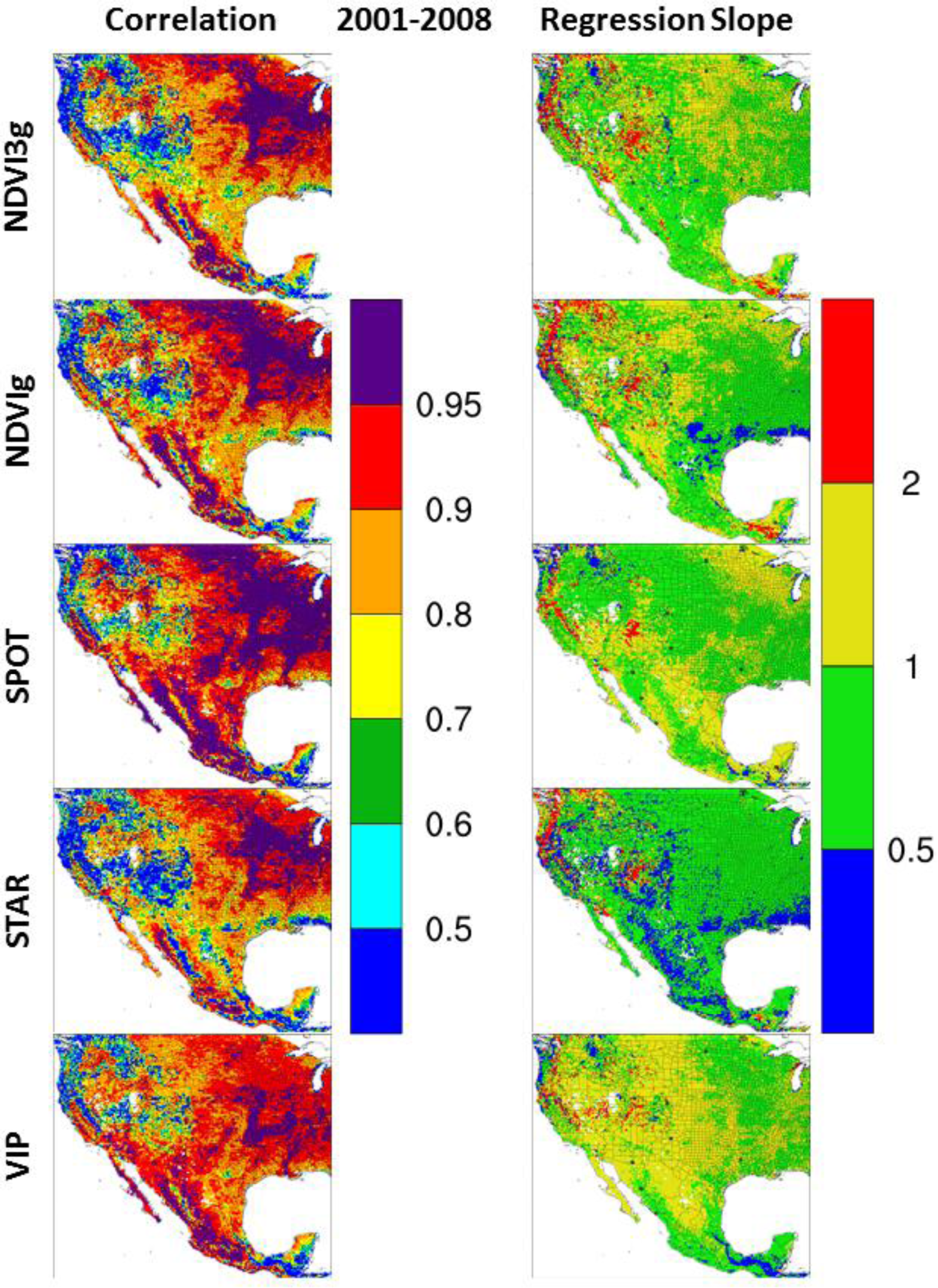
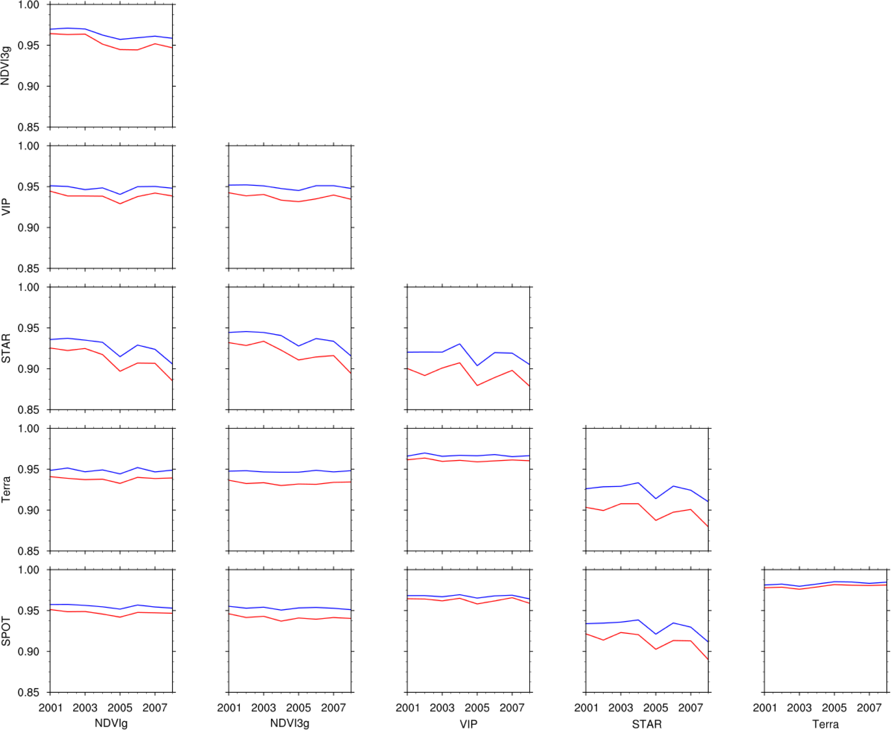
3.1. NDVI Intercomparison

For the regression using all time periods over the 9 locations between 2001 and 2008, the correlations are higher than 0.9 between all products; however variations in correlations do exist (Figure 1). As expected the SPOT NDVI is correlated highest with Terra (0.97) as the sensors behind these two datasets have a higher spectral resolution and the NIR and red bands were designed for more appropriate vegetation monitoring than the AVHRR sensor. The NDVI datasets based on these sensors have also been shown to be more highly correlated to high-resolution ground-based [39] and Landsat NDVI [36] than the AVHRR-based NDVIg. There are also variations in the regression slopes between the products. Most comparisons between datasets have slopes near 1. Terra, VIP, and NDVI3g tend to have higher values compared to SPOT, NDVIg, and STAR. Even though the slope between Terra and NDVI3g is greater than one, the y-intercept indicates that NDVI3g has on average slightly larger NDVI values, which is consistent with results from Fensholt and Proud [23]. STAR NDVI values are substantially lower than all other products, because STAR is the only AVHRR-based dataset that has not been adjusted to match the range of MODIS as has been done with NDVIg, NDVI3g and VIP.

Past research has shown that while AVHRR [58] and SPOT [38] ground-based NDVI sensors correlate very highly with MODIS sensors, the satellite-based correlations are lower and regression slopes exhibit large departures from one, suggesting that atmospheric correction is not as robust for the AVHRR and SPOT satellite-based NDVI than MODIS satellite-based NDVI. The lower correlation of STAR with Terra than those of NDVIg and NDVI3g with Terra could be due to a lack of atmospheric corrections used in STAR.

The general relationships shown in Figure 1 vary significantly in space (Figure 2). In general, most individual points have a correlation lower than what was found in the 9-point correlation in Figure 1. While there are large areas with high correlations between products above 0.90, there are also locations where correlations are much lower. All products tend to have lower correlations when compared to Terra from the Rocky Mountains westward in the United States and in the evergreen broadleaf forests of southeastern Mexico. The three products based purely on AVHRR NDVI (NDVI3g, NDVIg, and STAR) have lower correlations with Terra over the Gulf Coast of the United States and northeastern Mexico. Based on the combination of AVHRR and MODIS data, VIP shows higher correlations in these areas than the other three AVHRR-based products, particularly over northeastern Mexico and the Southwest US SPOT shows the highest correlations of all products east of the Rocky Mountains, in the Southwest US and in the northern two-thirds of Mexico.

Previous research suggests similar spatial variations in correlation and regression slopes between NDVIg and MODIS [37] and between NDVI3g and MODIS [23]. However the analysis of Fensholt and Proud [23] showed slightly lower correlations over the northern Rocky Mountains of the USA.

While the correlations for NDVI between each product and Terra were relatively similar, the regression slopes are quite different in their spatial patterns (Figure 2) consistent with the differences seen in Figure 1. NDVI3g has a greater area of slopes less than one than area with slopes greater than one, but there are very high slopes greater than 2 over some areas (e.g., mountainous areas along the west coast of the US, the Mogollon Rim in northern Arizona, and parts of southeastern Mexico) which is consistent with recent research [23]. NDVIg has a similar spatial pattern except for lower slopes (less than 0.5) in parts of the Mexican Plateau, southern Texas and the southeastern US There is a smaller area of slopes greater than 2 or less than 0.5 from SPOT and VIP than from NDVIg or NDVI3g indicating that the relationship of SPOT and VIP with Terra is more uniform in space than Terra’s relationship with NDVI3g and NDVIg. Additionally, over most of the area, the slope of the relationship between STAR and Terra is less than 1.

There are also significant temporal changes in the relationship between products. Figure 3 shows that the spatial correlations for NDVI (blue) remain above 0.85 over all times among all products and above 0.95 among VIP, SPOT, and Terra. The correlations between STAR and all other products are the lowest, and they also show a negative trend with time. The reasons for these trends are unknown at present and need to be explored in the future. Also, there are seasonal variations in correlations (not-shown) that generally show a late spring-summer maximum and a late fall-winter minimum. Figure 4 shows how the spatial regression slopes in NDVI changed from 1982 to 2008 between the four long-term datasets. NDVIg and NDVI3g have a fairly stable relationship through time, because they are different versions of the product from the same group. VIP shows strong interannual changes in the regression slopes with both NDVIg and NDVI3g. The strongest changes coincide with a change from using AVHRR data to using MODIS data in the year 2000. Between 2001 and 2008 the relationship between VIP and NDVIg and NDVI3g is virtually the same as the relationship between Terra and NDVIg and NDVI3g (shown by green line) which is evidence of the strong relationship between VIP and MODIS. Also, consistent with Figures 1 and 2, STAR has very low regression slopes with the other 3 datasets.

The interannual mean and range of N_p,max is explored in

Table 2. Comparison of six datasets (T-Terra, SP-SPOT, g-NDVIg, 3g-NDVI3g, ST-STAR, V-VIP) of the interannual mean and range of the maximum annual NDVI (N_p,max) and the maximum annual green vegetation fraction (MGVF) for each IGBP land cover class and all land pixels (Total) from 2001 to 2008. The average over all pixels was first calculated before the interannual mean and range were computed. The number of 0.125° pixels for each land cover class is in parentheses.

		Np,max						MGVF
IGBP Type		T	SP	g	3g	ST	V	T	SP	G	3g	ST	V
Mean
1	ENFor (3347)	0.75	0.71	0.70	0.85	0.49	0.81	0.89	0.88	0.89	0.90	0.86	0.90
2	EBFor (1463)	0.85	0.81	0.76	0.87	0.50	0.86	0.94	0.96	0.91	0.93	0.90	0.95
3	DNFor (0)
4	DBFor (696)	0.86	0.81	0.81	0.89	0.56	0.89	0.96	0.96	0.95	0.95	0.92	0.97
5	MixFor (3062)	0.82	0.77	0.76	0.88	0.52	0.86	0.94	0.93	0.92	0.94	0.90	0.95
6	ClsShr (149)	0.58	0.52	0.56	0.65	0.36	0.65	0.83	0.84	0.86	0.86	0.83	0.86
7	OpnShr (8609)	0.36	0.31	0.33	0.39	0.22	0.41	0.46	0.44	0.45	0.47	0.46	0.49
8	WdySav (4562)	0.77	0.71	0.71	0.82	0.47	0.81	0.91	0.91	0.90	0.91	0.90	0.93
9	Sav (132)	0.66	0.60	0.60	0.78	0.44	0.73	0.92	0.92	0.93	0.94	0.92	0.94
10	Grass (19449)	0.50	0.44	0.49	0.57	0.32	0.57	0.76	0.73	0.77	0.77	0.76	0.78
11	Wetlnd (84)	0.56	0.60	0.50	0.63	0.32	0.66	0.72	0.81	0.69	0.75	0.70	0.78
12	Crop (8592)	0.75	0.69	0.73	0.81	0.49	0.80	0.87	0.86	0.87	0.90	0.86	0.89
13	Urban (347)	0.52	0.46	0.49	0.65	0.35	0.59	0.73	0.70	0.69	0.74	0.68	0.73
14	CrpVeg (4959)	0.79	0.74	0.75	0.86	0.52	0.83	0.93	0.93	0.92	0.94	0.91	0.95
16	Barren (543)	0.15	0.13	0.16	0.20	0.11	0.18	0.12	0.11	0.14	0.19	0.17	0.14
	Total (55994)	0.61	0.55	0.58	0.67	0.39	0.66	0.77	0.76	0.77	0.79	0.77	0.79
Range
1	ENFor	0.03	0.03	0.04	0.02	0.03	0.03	0.01	0.01	0.01	0.01	0.03	0.01
2	EBFor	0.01	0.04	0.02	0.02	0.04	0.02	0.01	0.01	0.02	0.01	0.01	0.01
3	DNFor
4	DBFor	0.02	0.04	0.05	0.03	0.04	0.02	0.01	0.02	0.01	0.01	0.02	0.01
5	MixFor	0.02	0.04	0.03	0.01	0.04	0.03	0.01	0.01	0.01	0.01	0.03	0.01
6	ClsShr	0.04	0.06	0.06	0.04	0.04	0.06	0.07	0.04	0.05	0.02	0.06	0.03
7	OpnShr	0.07	0.11	0.06	0.04	0.06	0.11	0.13	0.12	0.10	0.05	0.10	0.13
8	WdySav	0.02	0.04	0.02	0.01	0.03	0.03	0.00	0.01	0.02	0.01	0.02	0.02
9	Sav	0.10	0.10	0.07	0.03	0.06	0.06	0.04	0.05	0.04	0.03	0.03	0.04
10	Grass	0.06	0.09	0.04	0.03	0.05	0.06	0.06	0.06	0.04	0.02	0.05	0.06
11	Wetlnd	0.06	0.04	0.02	0.02	0.04	0.06	0.05	0.02	0.02	0.02	0.07	0.05
12	Crop	0.03	0.06	0.02	0.02	0.05	0.02	0.02	0.03	0.02	0.02	0.04	0.02
13	Urban	0.03	0.04	0.02	0.02	0.03	0.02	0.02	0.02	0.03	0.02	0.03	0.02
14	CrpVeg	0.02	0.04	0.02	0.01	0.04	0.02	0.01	0.01	0.01	0.01	0.01	0.01
16	Barren	0.07	0.10	0.06	0.06	0.04	0.09	0.11	0.12	0.09	0.09	0.10	0.13
	Total	0.03	0.07	0.02	0.02	0.04	0.04	0.04	0.04	0.03	0.02	0.03	0.04

. Also, the mean and range of the maximum annual green vegetation fraction (MGVF) is shown and will be discussed in Section 3.3. The highest means of N_p,max are seen in the deciduous broadleaf forest, evergreen broadleaf forest, mixed forest, woody savannah and mixed cropland vegetation areas. The lowest N_p,max are seen in the barren and open shrubland classes. There are significant N_p,max differences between datasets in magnitude with the highest (or lowest) N_p,max values from NDVI3g (or STAR) on average. The interannual ranges of N_p,max for most classes vary between 0.02 and 0.04 with noticeably higher ranges for SPOT N_p,max in most classes. The largest interannual variations are seen in open and closed shrublands, barren areas and savannah. Also, grasslands and wetlands have moderate to high ranges. NDVI3g has both the lowest interannual range for all land pixels as well as lower ranges for most land cover classes. Furthermore, NDVI3g has better calibration and inter-sensor alignment than NDVIg and this is likely one of the reasons for the lower interannual variability [59].

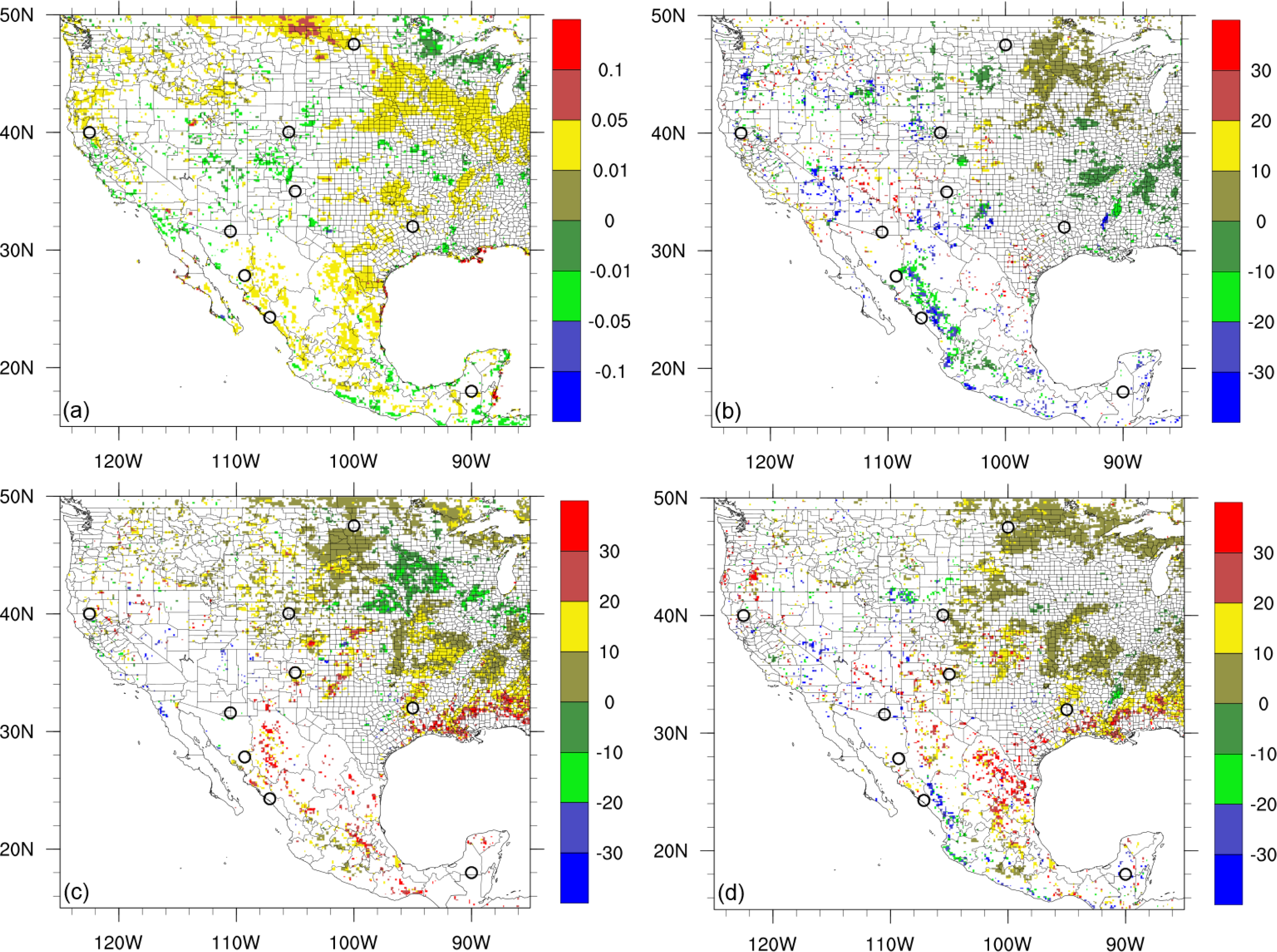
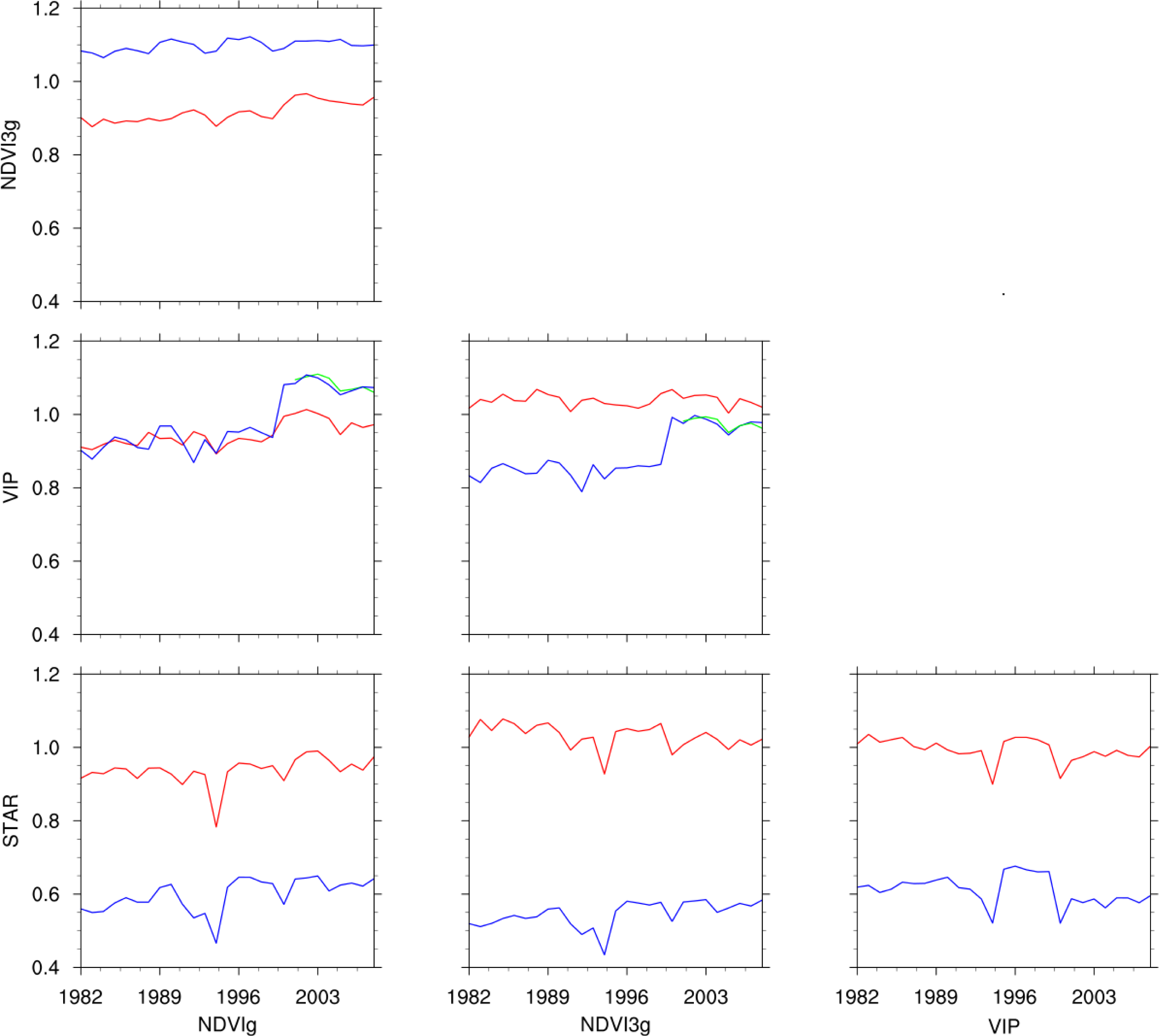
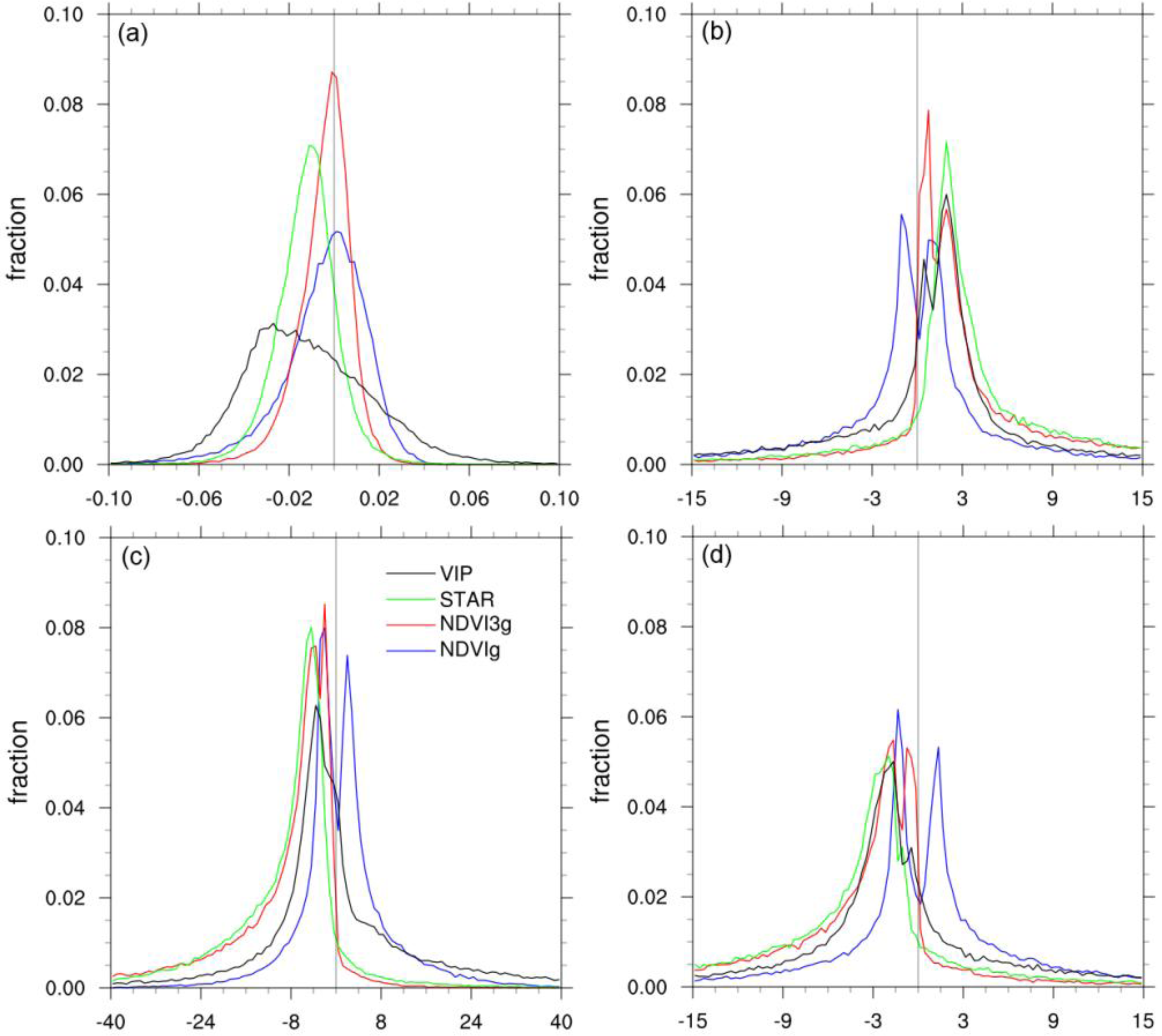
3.2. NDVI Trend Intercomparison

The trends of N_p,max and NDVI phenology are compared to determine how effective the long-term datasets are in detecting vegetation trends. Figure 5 shows the interannual trends of the maximum annual NDVI (N_p,max), start of season, end of season, and duration of season for NDVI3g. Trends near the border with Canada in western North Dakota and eastern Montana as well as trends in the Corn Belt of southern Minnesota, northern Iowa, Illinois and much of northern Mexico suggest a positive trend in N_p,max (Figure 5a). Past studies analyzing long-term changes in NDVI-based vegetation abundance across the area vary based on the dataset being used as well as the method of estimation. For instance, Forzieri et al. [27] using NDVIg shows a strong significant increase in N_p,max over areas of N. Central Mexico that are not apparent in NDVI3g from Figure 5a or VIP and STAR (not shown). Several studies agree with increasing annual NDVI in the border region of North Dakota, eastern Montana and Canada [36,60,61]. Furthermore, Beck et al. [36] found large disagreements between various AVHRR-based long-term NDVI datasets over the Southeast US and lower Missouri Valley region, suggesting that care should be taken in interpreting trends in these areas. De Jong et al. [61] showed that nearly all pixels across US/Mexico have seen at least one major change in trend.

A significant trend in start of season is seen in the Sierra Madre Occidental and Southwestern Mexico where the season is beginning up to 10 days earlier per decade (Figure 5b). Also, there is a small trend towards delayed start over the Upper Midwest. Large areas of the northern US and Southeast US show significant delays in the end of season with the exception being over the Corn Belt of Northern Iowa and Illinois (Figure 5d). Trends vary over Mexico, suggesting an earlier end of season in southwestern Mexico and a delayed end of season over the northeastern portion of Mexico. The combined results of trends in start and end of season show that deciduous broadleaf forests and mixed forests of the Lower Mississippi Valley and Southeast US are seeing a longer season (Figure 5c). There are also trends in the western Great Lakes region and Dakotas outside of the corn belts towards a longer greening period as well, whereas over the Corn Belt the season is decreasing in duration. Over Mexico, there are no obvious areas of significant trends but most significant pixels suggest an increase in season duration.

Results from Fensholt et al. [59] suggested that over North Dakota and South Dakota the maximum NDVI is increasing while the greening period duration is decreasing due both to delayed start and earlier end. These results are similar for the eastern Dakotas in our results in the northwestern portion of the Corn Belt. This might be the result of expansion of corn into this area which generally has a shorter greening period than natural areas. Jeong et al. [62] depicted a delayed onset over the Upper Midwest and central Plains, which is similar to the results presented here. However, our results tend to be more restrictive in the significance test masking more areas. For end of season most temperate areas over the US except the Corn Belt show delayed end of season and the duration of season is getting longer in the areas of delayed end of season. This result is mostly due to warmer summer and autumn temperatures. Julien and Sobrino [20] studied trends in phenology using a double logistic function fit to each year’s annual cycle and shows similar results with a few areas showing up as significant that are masked areas in this study.

Figure 6 shows histograms of the difference between each dataset and NDVI3g for the same NDVI-based phenology trends discussed for Figure 5. For all four phenology variables NDVIg doesn’t have a strong apparent bias in trends compared to NDVI3g but there are still many pixels with large differences. VIP and STAR each has a positive trend difference for N_p,max compared to NDVI3g. Regarding onset, VIP and STAR are nearly identical with trends towards earlier onsets than NDVI3g. The retreat is the opposite where both VIP and STAR have more delayed end of season dates than NDVI3g. The difference in trend for duration of season tends to integrate both the earlier start and delayed end of season for VIP and STAR, resulting in a positive trend difference of around 1 day per year. Despite these clear differences there is still a large range of differences, suggesting that many pixels for each product have both more positive and more negative trends for each phenology variable.

The change in NDVI-based phenology per land cover class for each product is shown in

Table 3. Comparison of 4 datasets (g-NDVIg, 3g-NDVI3g, ST-STAR, V-VIP) in the trends of the interannual maximum annual NDVI (N_p,max), NDVI greening period duration, start date, and end date for each IGBP land cover class and all land pixels (Total) from 1982 to 2008. Significant negative trends (italics) and positive trends (bold) were estimated using a t-test (with a 95% confidence level).

		Np,max (per decade)				Duration of Season (days/decade)				Start of Season (days/decade)				End of Season (days/decade)
IGBP Type		g	3 g	ST	V	g	3 g	ST	V	g	3 g	ST	V	g	3 g	ST	V
1	ENFor	−0.012	0.003	0.011	−0.015	−1.1	7.7	17.1	−11.7	9.9	6.2	−5.2	2.0	2.0	1.6	11.0	−3.0
2	EBFor	0.002	−0.001	0.016	0.031	−12.5	3.0	31.3	42.4	−2.8	−4.0	7.8	−5.0	−20.1	−11.2	26.3	16.5
3	DNFor
4	DBFor	−0.014	−0.003	0.015	0.028	4.9	5.9	15.6	15.2	−0.7	−2.1	−4.1	−6.0	4.7	4.5	10.6	8.1
5	MixFor	−0.011	−0.001	0.013	0.016	6.2	7.5	21.2	17.6	1.6	1.4	−2.1	−3.9	8.9	7.9	15.9	12.2
6	ClsShr	−0.004	0.000	0.009	−0.010	−2.9	1.5	23.8	−10.6	32.6	22.3	35.7	11.2	27.2	22.0	−55.2	−10.1
7	OpnShr	0.014	0.001	0.009	−0.009	3.8	3.9	13.9	−17.8	25.3	13.2	33.2	14.3	29.1	14.8	42.7	−6.2
8	WdySav	−0.002	0.004	0.021	0.026	7.2	10.0	31.8	24.1	−2.7	−1.5	−4.0	−7.9	9.1	8.1	26.3	15.5
9	Sav	−0.005	−0.004	0.009	0.013	−11.6	0.9	17.1	11.8	−0.3	−0.7	−7.2	−21.3	−17.0	−0.4	13.8	−7.2
10	Grass	0.009	0.002	0.009	0.009	3.5	3.7	16.3	7.8	0.3	0.8	−2.4	−3.6	4.6	4.4	13.0	5.0
11	Wetlnd	−0.003	−0.001	0.019	0.031	16.2	13.9	30.2	20.7	−4.5	−2.6	−11.2	−6.9	20.2	14.8	25.4	11.2
12	Crop	0.014	0.014	0.021	0.036	1.2	0.5	13.0	11.5	1.8	1.7	−2.4	−4.5	2.4	1.5	8.5	6.0
13	Urban	−0.010	−0.001	0.000	−0.012	−3.1	−0.3	11.5	−5.2	2.4	2.6	−1.7	0.9	2.3	2.3	12.1	1.4
14	CrpVeg	−0.008	0.002	0.015	0.029	2.3	4.9	18.0	18.8	−0.7	−0.6	−3.1	−6.8	3.2	3.7	10.5	8.1
16	Barren	0.005	−0.001	0.000	−0.024	0.9	−1.3	−1.5	−33.2	−7.3	−16.2	−13.2	32.7	−4.4	−4.5	−1.2	15.3
	Total	0.005	0.004	0.013	0.013	2.7	4.2	17.5	7.6	3.0	2.2	0.2	−3.4	7.1	5.7	13.9	5.0

. For N_p,max, only cropland shows significant and unanimous increases over the past 27 years among the four products. The only other category that has unanimous agreement is grassland which only has one significantly increasing dataset. There is also broad agreement in a general increase in N_p,max averaged across all land classes. Trends in the start of season are inconsistent across most classes with some consensus over a delayed start over the open and closed shrublands and an earlier start over deciduous broadleaf, mixed cropland vegetation and wetlands. The trends over semi-arid areas should be interpreted with caution since these areas have a multi-modal annual greening cycle. The end of season shows a general consensus over the total of all classes and most individual classes of a delay in the end of season. Mixed forest, deciduous broadleaf, woody savannah and wetland classes show unanimous significantly delayed ends to the greening period. The duration of season for most classes is trending towards longer seasons and is impacted most strongly by the end of season although there is weaker agreement. Jeong et al. [62] showed a general result that while Europe and Asia have seen more balanced increases in duration of greening period with earlier onsets and delayed senescence, the US has seen most increases in season duration due to a delayed end of season. This agrees well with our study in the forested areas of the lower Mississippi Valley, the Southeast US and the western Great Lakes region.

The current NDVI comparison was performed using version 2 of the VIP dataset. The new version (VIP V3) has recently been released (December 2013) and has addressed problems associated with higher NDVI in sparsely vegetated areas prior to 2000. It has also addressed gap filling issues over areas that are covered with snow during the winter and has reduced NDVI error by around 2% in the summer maximum NDVI signal [63]. Future work should compare the version used here (V2) with the new version (V3) to determine how our analysis would change.

3.3. Calculation of Green Vegetation Fraction

The analyses of NDVI datasets and interannual phenology trends in Sections 3.1 and 3.2 show that there are significant differences in mean value and trend between the various datasets. While the easiest way would be to interpret these differences as the uncertainties of these datasets, a more interesting question is: Can we find a way to reduce these uncertainties? Here we address this issue using the Green Vegetation Fraction (GVF) algorithm from [41,42] that is dependent on land cover type and is independent of spatial resolution of the data:

$$\mathit{GVF}=\frac{N-N_s}{N_{c,v}-N_s}$$

(1)

where N is the NDVI for each pixel and time period, N_s is the bare ground NDVI computed annually and N_c,v is the NDVI that corresponds to 100% GVF calculated annually for each land cover. The MODIS 0.5 km Land Cover (MCD12Q1) from 2004 was upscaled to the 0.125° grid and the most frequent type of all MODIS pixels within each coarse grid cell was used as the land cover type. First, the maximum annual NDVI (N_p,max) is calculated for each pixel then the histograms of N_p,max for all pixels of each land cover are calculated and the 75th percentile of most types and 90th percentile of closed shrubland and urban classes are used as the N_c,v for a given land cover class. The N_c,v of open shrubland and barren is prescribed the N_c,v of the closed shrubland class because these classes may not have any pixels that have reached full capacity or 100% GVF. The value of Nc,v, particularly for forest classes, was shown to be insensitive to percentile used in Zeng et al. [41]. N_s is calculated as the 5th percentile of N_p,max for the Barren class. Finally, GVF is constrained within 0 and 1. Physically, NDVI values greater than N_c,v should represent vegetation with higher leaf area index (LAI) or healthier vegetation and not a higher areal coverage of vegetation. More details on the GVF computation are provided in [41,42].

There are three assumptions underlying this formulation of GVF. First, this method assumes that all seasonal changes in NDVI are due to changes in GVF alone or in the concurrent changes of GVF and LAI. Changes in NDVI are not only due to changes in the fraction of green vegetation, but also LAI, vegetation health among other factors. Therefore GVF should be understood as a combination of factors that lead to higher overall vegetation greenness. The second assumption is that the bare soil in each pixel can be represented by one value N_s and the 100% GVF NDVI of each pixel can be represented by one value N_c,v based on a pixel’s dominant land cover. In reality, the area of a pixel that is not green vegetation can be represented by soil of different textures and soil moistures, leaf litter, and dormant vegetation. The green vegetation for a given land cover would ideally be represented by the same combination of vegetation for each pixel but in reality even within the same class the composition of vegetation would vary, not to mention that pixels often are composed of other non-dominant vegetation classes. This assumption would be most valid in the interior of a land cover class. The final assumption is that the interannual variations of N_c,v and N_s are due to spurious changes in NDVI that result from errors contained within the NDVI datasets and that they are not due to true changes in the surface NDVI.

In order to check for the temporal consistency in N_p,max and validate the utility of calculating N_c,v and N_s separately each year, we analyzed the time-series of N_c,v for each land cover category as well as N_s for each of the long-term NDVI products from 1982–2008 (not shown). For the VIP product, jumps in N_s as well as N_c,v are evident and occur at the year 2000 when this product switches to using MODIS as the main source of information for NDVI. Prior to 2000, N_s was more variable and averaged 0.12; whereas, afterwards, N_s was stable and around 0.1. Decreases in N_c,v were seen for evergreen needleleaf, shrublands, and grasslands, while increases were seen for deciduous broadleaf and mixed forests. Similar but less apparent jumps occur in other products as well at this same time including a noticeable increase in N_s for NDVI3g from 0.05 to 0.08 and decreases in the N_c,v of many land cover classes for STAR. Also, the interannual values of N_c,v are much more stable for NDVI3g than the other three products. It’s very challenging to identify the true variability of vegetation, the use of N_c,v and N_s each year helps to remove some of the spurious variability (jump) but a more rigorous approach is still needed to identify the true variability in the future.

In comparison to the original NDVI relationships between products shown in Figure 1, nearly all of the derived GVF relationships are much closer to one-to-one (Figure 7). On the other hand, all correlations between products were reduced slightly. This slight reduction is also evident in the time-series of spatial correlations for GVF in Figure 3. Similar to Figure 7, the time series of the spatial regression slope in GVF is much closer to 1 than that for NDVI itself (Figure 4). Furthermore, the GVF relationship between VIP and NDVI3g is much more stable with time (than that of NDVI) and the relationship between VIP and NDVIg is slightly more stable, suggesting a correcting influence of GVF on relationships between products each year.

Table 2 shows how the interannual mean and range in MGVF vary across the six datasets over all pixels for each IGBP land cover class. In comparison to N_p,max which was discussed earlier, most land cover classes have a higher average MGVF. The largest increases were seen over the closed shrublands, savannah, and grassland classes. More importantly the MGVF across different datasets for each given class are much more uniform than N_p,max, showing how well GVF normalizes the values. The interannual variation expressed through the range in Table 2 suggests reduced variation in MGVF for most classes in comparison to N_p,max.

The results from Zeng et al. [14] compare very similarly to Table 2. The largest differences are in classes where there wasn’t much data in this study such as savannah, closed shrublands, and wetlands which tend to have lower mean MGVF than this study. The ranges are also similar in most classes except larger ranges in open shrublands and barren classes. While the large range in this study is not surprising, it’s uncertain why the global study of Zeng et al. [14] has reduced barren interannual variability. One possible reason is that areas of barren land throughout North America are fairly isolated and hence may include some very sparse open shrubland areas, whereas other areas on Earth such as Africa and Asia have large barren deserts that only change at the margins.

3.4. GVF to NDVI Trend Changes

Histograms of the difference between GVF- and NDVI-based phenology trends are shown in Figure 8. Trends are more negative for MGVF than N_p,max for all datasets (particularly VIP and STAR) (Figure 8a). GVF-based trends in start of season tend to be more positive for VIP, STAR and NDVI3g (Figure 8b) whereas for end of season they tend to be more negative (Figure 8d). These result in more negative duration of season trends for GVF versus NDVI (Figure 8c) and suggest that GVF-based phenology trends in duration of season are weaker than the original NDVI-based trends.

In order to compare to the NDVI-based phenology,

Table 4. Comparison of 4 datasets (g-NDVIg, 3g-NDVI3g, ST-STAR, V-VIP) in the trends of the interannual maximum annual green vegetation fraction (MGVF), GVF greening period duration, start date, end date for all IGBP land cover classes and all land pixels (Total) from 1982 to 2008. Significant negative trends (italics) and positive trends (bold) were estimated using a t-test (with a 95% confidence level).

		MGVF (per decade)				Duration of Season (days/decade)				Start of Season (days/decade)				End of Season (days/decade)
IGBP Type		g	3 g	ST	V	g	3 g	ST	V	g	3 g	ST	V	g	3 g	ST	V
1	ENFor	0.000	−0.002	0.001	0.005	12.1	−1.0	8.2	17.0	0.3	5.9	4.0	−5.3	8.7	−1.8	7.2	11.8
2	EBFor	−0.001	−0.001	0.010	0.006	−16.1	1.2	18.5	4.3	−1.6	−3.7	20.2	15.6	−21.5	−11.7	22.6	4.5
3	DNFor
4	DBFor	0.003	0.001	0.013	0.008	9.6	5.6	12.0	10.7	−2.4	−2.0	−2.8	−4.4	6.6	4.4	8.8	6.2
5	MixFor	0.004	0.001	0.012	0.011	15.1	6.6	17.0	15.6	−1.4	1.6	−0.5	−3.2	13.4	7.3	13.6	11.2
6	ClsShr	−0.001	−0.006	−0.001	0.013	4.0	−7.9	8.9	21.5	30.4	23.8	42.1	−2.4	31.1	12.5	25.1	13.3
7	OpnShr	0.029	−0.011	0.005	0.011	9.2	−17.6	4.6	0.9	25.2	20.0	35.9	5.4	32.6	4.0	46.9	4.7
8	WdySav	0.004	0.001	0.012	0.007	11.3	4.0	16.0	11.4	−3.6	−0.3	−1.1	−4.2	10.9	5.2	15.5	9.1
9	Sav	0.005	−0.004	0.003	0.003	−4.0	−0.7	13.7	9.5	−3.2	0.3	−7.6	−18.9	−10.1	−1.0	5.6	−7.0
10	Grass	0.010	−0.009	0.006	0.002	0.4	−8.3	8.2	5.7	1.8	5.2	1.1	−2.5	3.1	−3.1	8.7	4.1
11	Wetlnd	0.002	−0.003	0.007	0.009	20.6	11.6	14.3	2.8	−5.0	−2.2	−7.6	−4.3	20.5	12.1	11.7	2.1
12	Crop	0.003	0.001	0.005	0.009	−2.8	−7.0	4.7	4.2	3.7	5.2	1.4	−1.0	0.5	−1.7	5.0	3.0
13	Urban	0.001	−0.004	−0.006	−0.014	8.2	−6.4	7.8	0.6	−1.9	4.6	−0.6	−1.2	8.9	−0.8	9.8	4.2
14	CrpVeg	0.001	0.002	0.007	0.008	6.4	2.5	11.8	10.6	−1.9	0.2	−0.9	−4.2	4.9	2.6	8.0	5.0
16	Barren	0.013	−0.021	−0.011	−0.014	6.8	−30.2	−10.0	−11.9	−23.2	10.4	−2.1	6.4	0.3	−30.1	−13.9	14.4
	Total	0.009	−0.005	0.006	0.006	3.9	−5.8	8.8	6.9	3.1	5.4	3.4	−2.5	7.5	0.7	10.1	4.8

shows how GVF-based phenology is changing per land cover class for each product. The differences between the NDVI- and GVF-based phenology trends (Tables 3 and 4) are large and similar in magnitude to the mean trend values. However, the overall results towards increased duration of season due to a delayed end of season over most vegetation classes remain the same for VIP, STAR, and NDVIg. For MGVF, deciduous broadleaf forests, mixed forests, woody savannah and mixed cropland-vegetation areas all have agreement on an increase in MGVF with at least 3 significant datasets (Table 4). While our study shows general agreement on positive trends in most vegetation classifications, the study of Zeng et al. [14] showed negative trends over evergreen forests, mixed forests and urban classes and positive and generally larger trends were seen over deciduous needleleaf, open shrubland, savannah, grassland, wetland and cropland classes. However, a direct comparison cannot be made since our study region only includes a small subset of the global analysis they completed.

4. Conclusions

In this study we have intercompared four long-term NDVI datasets and three shorter-term NDVI datasets based on newer sensors. The correlation between NDVI products based on the two new sensors (MODIS and SPOT) is higher than that between AVHRR-based products or between AVHRR- and MODIS/SPOT-based products. Most regression slopes are close to 1 among all products; however, STAR is consistently lower than all other NDVI datasets.

The spatial variation in temporal correlation shows that most areas are well correlated; however, lower correlations occur in arid and mountainous regions. There are also large spatial variations in regression slopes between various products but the patterns of these variations depend on the specific products being compared. Temporal variation in the spatial correlation of NDVI shows high correlations above 0.8 for the entire time period with the lowest correlations between STAR and other datasets. Long-term datasets show significant changes in regression slopes through time especially between VIP and other datasets due to VIP’s changing dependence from AVHRR before 2000 to MODIS afterwards. With respect to land cover classes, there are significant inter-product differences in mean N_p,max but interannual variation in N_p,max is fairly low (0.02 to 0.04) for most vegetation classes with the exception of more sparsely vegetated shrublands, grasslands and barren areas.

Trend analyses of N_p,max and NDVI-based phenology for the four long-term datasets suggest that trends in N_p,max from NDVI3g are positive for most pixels with significant trends at the 95% confidence level. An increasing trend in duration of season mostly due to a delay in the end of season is apparent over much of the US east of the Rocky Mountains with the exception of agricultural areas such as the Corn Belt. Also, results suggest an earlier start of season over the Sierra Madre Occidental area of Mexico. Histograms of differences in NDVI phenology trends suggest VIP and STAR are characteristic of more positive trends in N_p,max and duration of season than NDVIg and NDVI3g. However, there are still many pixels that show more negative trends as well, suggesting a lot of spatial variation in the difference of trends. In most temperate vegetation classes the trend is towards a delayed end of season across all products.

A method of normalizing NDVI using GVF was tested to determine if the GVF-derived datasets are better related and produce more uniform trends than the original NDVI datasets. The results showed that the change to GVF creates more one-to-one temporal and spatial relationships between products and long-term changes in these relationships are minimized compared to original NDVI relationships. Overall, there is a slight reduction in temporal correlation; however, spatial correlations increase between most products. When looking at different LC classes, MGVF is higher than N_p,max, more uniform across different datasets and there is less interannual range.

In general, the magnitude of MGVF changes are reduced compared to N_p,max changes east of the Rocky Mountains. Trends in both MGVF and GVF-based phenology are weaker and closer to each other across products than for NDVI. The results for trends in GVF-based phenology across LC classes are similar to NDVI-based trends but generally weaker with less agreement across datasets especially for MGVF trends.

There are a few implications that result from this study. Due to the high inter-product correlation and better trend agreement, more consistent conclusions are expected for vegetation studies over deciduous forest areas; whereas, over evergreen, arid and mountainous regions results are less reliable. Also, because there are still significant disagreements between different NDVI datasets and the derived GVF datasets regarding seasonal and interannual variability, one should be cautious in drawing any conclusions regarding the long-term trend of vegetation coverage and phenology if only one satellite-based vegetation dataset is used. However, it’s not always practical to use multiple datasets. For studies that use a single dataset, important trends should be checked against some other form of data such as in-situ or modelled vegetation data [64] to confirm hypotheses. The transformation of NDVI into GVF using the method described here created more homogeneous datasets that can each be compared to physical model variables and provide multiple instances of validation to a single model. Furthermore, they can be used to force vegetation changes in models that don’t have dynamic vegetation. Finally, while some work has been done on creating regional [65] and global [51] multi-sensor NDVI synthesis products, in order to create datasets more capable of validating and calibrating dynamic vegetation models, the goal of the satellite vegetation community should be to create a vegetation dataset that estimates real vegetation quantities such as green vegetation fraction, vegetation health, leaf area index, fPAR and biomass, and identifies the uncertainty of all values for each time period and pixel once systematic errors have been removed.

While the current study broadly compared several recent NDVI datasets and the usefulness of GVF in homogenizing them, a series of more targeted studies need to be undertaken to fully understand the differences that exist between various datasets. The most important limitation of this study is that there was no validation against data that could serve as a “ground truth”. In order to make a value judgment on how well each product performs under various situations, future studies should validate datasets against in-situ vegetation measurements, flux tower observations, and high resolution remote sensing including satellite images and field scale photography. Possible underlying reasons for dataset differences need to be explored, including different methods of correcting atmospheric effects such as water vapor, clouds and aerosols, different spatial and temporal compositing methods used, different spectral response functions of the sensors, and orbital and sensor degradation.

Another limitation to this study was the simple threshold-based phenology detection. A more robust methodology is needed to track phenology changes in arid and evergreen areas which often have multiple growing seasons, limited seasonal vegetation range, and interannual variations in vegetation that can be stronger than seasonal variations. A more critical analysis of trends and the interannual variability of datasets is needed. Are interannual trends linear or are these trends changing over time? Do datasets have similar modes of variability? Furthermore, the root cause of such variability needs to be determined separating out real vegetation variations from those due to systematic errors or uncertainties in the datasets. Variability of these datasets should be compared to ground truth as well as modelled vegetation variability driven by observed climate changes, fires, diseases and land-use change.

A good understanding of the causes behind interannual variability will also help in determining the best method of computing the GVF and/or other biophysical variables based on satellite vegetation indices. In future studies the GVF should be based on N_c,v and N_s derived from histograms of N_p,max for all pixels across the globe for each land cover class rather than the regional data used here. Furthermore, experimental work is needed to determine the true relationship between GVF and NDVI, and how vegetation NDVI and bare soil NDVI vary in space and time, using data from the highest resolution to the coarser satellite data used in this study.

References

1. Hansen, A.J.; Neilson, R.P.; Dale, V.H.; Flather, C.H.; Iverson, L.R.; Currie, D.J.; Shafer, S.; Cook, R.; Bartlein, P.J. Global change in forests: Responses of species, communities, and biomes. Bioscience 2001, 51, 765–779. [Google Scholar]
2. Jackson, R.B.; Banner, J.L.; Jobbagy, E.G.; Pockman, W.T.; Wall, D.H. Ecosystem carbon loss with woody plant invasion of grasslands. Nature 2002, 418, 623–626. [Google Scholar]
3. Walther, G.-R.; Post, E.; Convey, P.; Menzel, A.; Parmesan, C.; Beebee, T.J.C.; Fromentin, J.-M.; Hoegh-Guldberg, O.; Bairlein, F. Ecological responses to recent climate change. Nature 2002, 416, 389–395. [Google Scholar]
4. Parmesan, C.; Yohe, G. A globally coherent fingerprint of climate change impacts across natural systems. Nature 2003, 421, 37–42. [Google Scholar]
5. Donohue, R.J.; Roderick, M.L.; McVicar, T.R.; Farquhar, G.D. Impact of CO2 fertilization on maximum foliage cover across the globe's warm, arid environments. Geophys. Res. Lett 2013, 40, 3031–3035. [Google Scholar]
6. Knapp, A.K.; Smith, M.D. Variation among biomes in temporal dynamics of aboveground primary production. Science 2001, 291, 481–484. [Google Scholar]
7. Deering, D. Rangeland Reflectance Characteristics Measured by Aircraft and Spacecraft Sensors; Texas A & M University: College Station, TX, USA, 1978. [Google Scholar]
8. Tucker, C. Red and photographic infrared linear combinations for monitoring vegetation. Remote Sens. Environ 1979, 8, 127–150. [Google Scholar]
9. Wang, Q.; Adiku, S.; Tenhunen, J.; Granier, A. On the relationship of NDVI with leaf area index in a deciduous forest site. Remote Sens. Environ 2005, 94, 244–255. [Google Scholar]
10. Sellers, P.J.; Tucker, C.J.; Collatz, G.J.; Los, S.O.; Justice, C.O.; Dazlich, D.A.; Randall, D.A. A revised land surface parameterization (SiB2) for atmospheric GCMS. Part II: The generation of global fields of terrestrial biophysical parameters from satellite data. J. Clim 1996, 9, 706–737. [Google Scholar]
11. Gutman, G.; Ignatov, A. The derivation of the green vegetation fraction from NOAA/AVHRR data for use in numerical weather prediction models. Int. J. Remote Sens 1998, 19, 1533–1543. [Google Scholar]
12. Defries, R.S.; Hansen, M.C.; Townshend, J.R.G.; Janetos, A.C.; Loveland, T.R. A new global 1-km dataset of percentage tree cover derived from remote sensing. Glob. Chang. Biol 2000, 6, 247–254. [Google Scholar]
13. Lu, H.; Raupach, M.R.; McVicar, T.R.; Barrett, D.J. Decomposition of vegetation cover into woody and herbaceous components using AVHRR NDVI time series. Remote Sens. Environ 2003, 86, 1–18. [Google Scholar]
14. Zeng, X.; Rao, P.; DeFries, R.S.; Hansen, M.C. Interannual variability and decadal trend of global fractional vegetation cover from 1982 to 2000. J. Appl. Meteorol 2003, 42, 1525–1530. [Google Scholar]
15. Nemani, R.R.; Keeling, C.D.; Hashimoto, H.; Jolly, W.M.; Piper, S.C.; Tucker, C.J.; Myneni, R.B.; Running, S.W. Climate-driven increases in global terrestrial net primary production from 1982 to 1999. Science 2003, 300, 1560–1563. [Google Scholar]
16. Baghzouz, M.; Devitt, D.A.; Fenstermaker, L.F.; Young, M.H. Monitoring vegetation phenological cycles in two different semi-arid environmental settings using a ground-based NDVI system: A potential approach to improve satellite data interpretation. Remote Sens 2010, 2, 990–1013. [Google Scholar]
17. Goetz, S.J.; Prince, S.D.; Goward, S.N.; Thawley, M.M.; Small, J.; Johnston, A. Mapping net primary production and related biophysical variables with remote sensing: Application to the BOREAS region. J. Geophys. Res. Atmos 1999, 104, 27719–27734. [Google Scholar]
18. Suzuki, R.; Nomaki, T.; Yasunari, T. Spatial distribution and its seasonality of satellite derived vegetation index (NDVI) and climate in Siberia. Int. J. Climatol 2001, 21, 1321–1335. [Google Scholar]
19. Myneni, R.B.; Tucker, C.J.; Asrar, G.; Keeling, C.D. Interannual variations in satellite-sensed vegetation index data from 1981 to 1991. J. Geophys. Res. Atmos 1998, 103, 6145–6160. [Google Scholar]
20. Julien, Y.; Sobrino, J.A. Global land surface phenology trends from GIMMS database. Int. J. Remote Sens 2009, 30, 3495–3513. [Google Scholar]
21. De Jong, R.; de Bruin, S.; de Wit, A.; Schaepman, M.E.; Dent, D.L. Analysis of monotonic greening and browning trends from global NDVI time-series. Remote Sens. Environ 2011, 115, 692–702. [Google Scholar] [Green Version]
22. Dahlke, C.; Loew, A.; Reick, C. Robust identification of global greening phase patterns from remote sensing vegetation products. J. Clim 2012, 25, 8289–8307. [Google Scholar]
23. Fensholt, R.; Proud, S.R. Evaluation of earth observation based global long term vegetation trends—Comparing GIMMS and MODIS global NDVI time series. Remote Sens. Environ 2012, 119, 131–147. [Google Scholar]
24. Beck, P.S.A.; Goetz, S.J. Satellite observations of high northern latitude vegetation productivity changes between 1982 and 2008: Ecological variability and regional differences. Environ. Res. Lett 2011. [Google Scholar] [CrossRef]
25. Salinas-Zavala, C.A.; Douglas, A.V.; Diaz, H.F. Interannual variability of NDVI in northwest Mexico. Associated climatic mechanisms and ecological implications. Remote Sens. Environ 2002, 82, 417–430. [Google Scholar]
26. Notaro, M.; Liu, Z.; Williams, J.W. Observed vegetation-climate feedbacks in the United States. J. Clim 2006, 19, 763–786. [Google Scholar]
27. Forzieri, G.; Castelli, F.; Vivoni, E.R. Vegetation dynamics within the North American monsoon region. J. Clim 2011, 24, 1763–1783. [Google Scholar]
28. Castro, C.L.; Beltrán-Przekurat, A.B.; Pielke, R.A. Spatiotemporal variability of precipitation, modeled soil moisture, and vegetation greenness in North America within the recent observational record. J. Hydrometeorol 2009, 10, 1355–1378. [Google Scholar]
29. Donohue, R.J.; McVicar, T.I.M.R.; Roderick, M.L. Climate-related trends in Australian vegetation cover as inferred from satellite observations, 1981–2006. Glob. Chang. Biol 2009, 15, 1025–1039. [Google Scholar]
30. Fensholt, R.; Rasmussen, K. Analysis of trends in the Sahelian “rain-use efficiency” using GIMMS NDVI, RFE and GPCP rainfall data. Remote Sens. Environ 2011, 115, 438–451. [Google Scholar]
31. Xu, L.; Myneni, R.B.; Chapin, F.S., III; Callaghan, T.V.; Pinzon, J.E.; Tucker, C.J.; Zhu, Z.; Bi, J.; Ciais, P.; Tømmervik, H.; et al. Temperature and vegetation seasonality diminishment over northern lands. Nat. Clim. Chang 2013. [Google Scholar] [CrossRef]
32. Wang, W.; Anderson, B.T.; Phillips, N.; Kaufmann, R.K.; Potter, C.; Myneni, R.B. Feedbacks of vegetation on summertime climate variability over the North American Grasslands. Part I: Statistical analysis. Earth Interact 2006, 10, 1–27. [Google Scholar]
33. Van Leeuwen, W.J.D.; Orr, B.J.; Marsh, S.E.; Herrmann, S.M. Multi-sensor NDVI data continuity: Uncertainties and implications for vegetation monitoring applications. Remote Sens. Environ 2006, 100, 67–81. [Google Scholar]
34. Fensholt, R.; Nielsen, T.T.; Stisen, S. Evaluation of AVHRR PAL and GIMMS 10-day composite NDVI time series products using SPOT-4 vegetation data for the African continent. Int. J. Remote Sens 2006, 27, 2719–2733. [Google Scholar]
35. Alcaraz-Segura, D.; Liras, E.; Tabik, S.; Paruelo, J.; Cabello, J. Evaluating the consistency of the 1982–1999 NDVI trends in the Iberian Peninsula across four time-series derived from the AVHRR sensor: LTDR, GIMMS, FASIR, and PAL-II. Sensors 2010, 10, 1291–1314. [Google Scholar]
36. Beck, H.E.; McVicar, T.R.; van Dijk, A.I.J.M.; Schellekens, J.; de Jeu, R.A.M.; Bruijnzeel, L.A. Global evaluation of four AVHRR-NDVI data sets: Intercomparison and assessment against Landsat imagery. Remote Sens. Environ 2011, 115, 2547–2563. [Google Scholar]
37. Brown, M.E.; Pinzón, J.E.; Didan, K.; Morisette, J.T.; Tucker, C.J. Evaluation of the consistency of long-term NDVI time series derived from AVHRR,SPOT-vegetation, SeaWiFS, MODIS, and Landsat ETM+ sensors. IEEE Trans. Geosci. Remote Sens 2006, 44, 1787–1793. [Google Scholar]
38. Fensholt, R.; Sandholt, I.; Stisen, S. Evaluating MODIS, MERIS, and VEGETATION vegetation indices using in situ measurements in a semiarid environment. IEEE Trans. Geosci. Remote Sens 2006, 44, 1774–1786. [Google Scholar]
39. Fensholt, R.; Rasmussen, K.; Nielsen, T.T.; Mbow, C. Evaluation of earth observation based long term vegetation trends—Intercomparing NDVI time series trend analysis consistency of Sahel from AVHRR GIMMS, Terra MODIS and SPOT VGT data. Remote Sens. Environ 2009, 113, 1886–1898. [Google Scholar]
40. Song, Y.; Ma, M.; Veroustraete, F. Comparison and conversion of AVHRR GIMMS and SPOT VEGETATION NDVI data in China. Int. J. Remote Sens 2010, 31, 2377–2392. [Google Scholar]
41. Zeng, X.; Dickinson, R.E.; Walker, A.; Shaikh, M.; DeFries, R.S.; Qi, J. Derivation and evaluation of global 1-km fractional vegetation cover data for land modeling. J. Appl. Meteorol 2000, 39, 826–839. [Google Scholar]
42. Miller, J.; Barlage, M.; Zeng, X.; Wei, H.; Mitchell, K.; Tarpley, D. Sensitivity of the NCEP/Noah land surface model to the MODIS green vegetation fraction data set. Geophys. Res. Lett 2006. [Google Scholar] [CrossRef]
43. Galvao, L.S.; Vitorello, I.; Pizarro, M.A. An adequate band positioning to enhance NDVI contrasts among green vegetation, senescent biomass, and tropical soils. Int. J. Remote Sens 2000, 21, 1953–1960. [Google Scholar]
44. Teillet, P.M.; Staenz, K.; William, D.J. Effects of spectral, spatial, and radiometric characteristics on remote sensing vegetation indices of forested regions. Remote Sens. Environ 1997, 61, 139–149. [Google Scholar]
45. Justice, C.O.; Eck, T.F.; Tanré, D.; Holben, B.N. The effect of water vapour on the normalized difference vegetation index derived for the Sahelian region from NOAA AVHRR data. Int. J. Remote Sens 1991, 12, 1165–1187. [Google Scholar]
46. Ignatov, A.; Laszlo, I.; Harrod, E.D.; Kidwell, K.B.; Goodrum, G.P. Equator crossing times for NOAA, ERS and EOS sun-synchronous satellites. Int. J. Remote Sens 2004, 25, 5255–5266. [Google Scholar]
47. Maisongrande, P.; Duchemin, B.; Dedieu, G. VEGETATION/SPOT: An operational mission for the Earth monitoring; presentation of new standard products. Int. J. Remote Sens 2004, 25, 9–14. [Google Scholar]
48. Huete, A.; Didan, K.; Miura, T.; Rodriguez, E.P.; Gao, X.; Ferreira, L.G. Overview of the radiometric and biophysical performance of the MODIS vegetation indices. Remote Sens. Environ 2002, 83, 195–213. [Google Scholar]
49. Tucker, C.J.; Pinzon, J.E.; Brown, M.E.; Slayback, D.A.; Pak, E.W.; Mahoney, R.; Vermote, E.F.; El Saleous, N. An extended AVHRR 8-km NDVI dataset compatible with MODIS and SPOT vegetation NDVI data. Int. J. Remote Sens 2005, 26, 4485–4498. [Google Scholar]
50. Jiang, L.; Kogan, F.N.; Guo, W.; Tarpley, J.D.; Mitchell, K.E.; Ek, M.B.; Tian, Y.; Zheng, W.; Zou, C.-Z.-Z.; Ramsay, B.H. Real-time weekly global green vegetation fraction derived from advanced very high resolution radiometer-based NOAA operational global vegetation index (GVI) system. J. Geophys. Res 2010, 115, 1–22. [Google Scholar]
51. Didan, K. Multi-Satellite Earth Science Data Record for Studying Global Vegetation Trends and Changes. Proceedings of the 2010 International Geoscience and Remote Sensing Symposium, Honolulu, HI, USA, 25–30 July 2010.
52. Barreto-Munoz, A. Multi-Sensor Vegetation Index and Land Surface Phenology Earth Science Data Records in Support of Global Change Studies: Data Quality Challenges and Data Explorer System. The University of Arizona, Tucson, AZ, USA, 2013. [Google Scholar]
53. Wang, D.; Morton, D.; Masek, J.; Wu, A.; Nagol, J.; Xiong, X.; Levy, R.; Vermote, E.; Wolfe, R. Impact of sensor degradation on the MODIS NDVI time series. Remote Sens. Environ 2012, 119, 55–61. [Google Scholar]
54. Holben, B.N. Characteristics of maximum-value composite images from temporal AVHRR data. Int. J. Remote Sens 1986, 7, 1417–1434. [Google Scholar]
55. Moody, A.; Strahler, A.H. Characteristics of composited AVHRR data and problems in their classification. Int. J. Remote Sens 1994, 15, 3473–3491. [Google Scholar]
56. White, M.A.; Thornton, P.E.; Running, S.W. A continental phenology model for monitoring vegetation responses to interannual climatic variability. Glob. Biogeochem. Cycles 1997, 11, 217–234. [Google Scholar]
57. Carroll, R.J.; Ruppert, D. The use and misuse of orthogonal regression in linear errors-in-variables models. Am. Stat 1996, 50, 1–6. [Google Scholar]
58. Fensholt, R.; Sandholt, I. Evaluation of MODIS and NOAA AVHRR vegetation indices with in situ measurements in a semi-arid environment. Int. J. Remote Sens 2005, 26, 2561–2594. [Google Scholar]
59. Myneni, R. Department of Earth and Environment, Boston University, Boston, MA. Personal Communication,. 2013.
60. Fensholt, R.; Langanke, T.; Rasmussen, K.; Reenberg, A.; Prince, S.D.; Tucker, C.; Scholes, R.J.; Le, Q.B.; Bondeau, A.; Eastman, R.; et al. Greenness in semi-arid areas across the globe 1981–2007—An earth observing satellite based analysis of trends and drivers. Remote Sens. Environ 2012, 121, 144–158. [Google Scholar]
61. De Jong, R.; Verbesselt, J.; Schaepman, M.E.; de Bruin, S. Trend changes in global greening and browning: Contribution of short-term trends to longer-term change. Glob. Chang. Biol 2012, 18, 642–655. [Google Scholar]
62. Jeong, S.-J.; Ho, C.-H.; Gim, H.-J.; Brown, M.E. Phenology shifts at start vs. end of growing season in temperate vegetation over the Northern Hemisphere for the period 1982–2008. Glob. Chang. Biol 2011, 17, 2385–2399. [Google Scholar]
63. Didan, K. Department of Electrical and Computer Engineering, The University of Arizona, Tucson, AZ. Personal Communication,. 2013.
64. Mao, J.; Shi, X.; Thornton, P.E.; Piao, S.; Wang, X. Causes of spring vegetation growth trends in the northern mid-high latitudes from 1982 to 2004. Environ. Res. Lett 2012. [Google Scholar] [CrossRef]
65. Zhang, G.; Zhang, Y.; Dong, J.; Xiao, X. Green-up dates in the Tibetan Plateau have continuously advanced from 1982 to 2011. Proc. Natl. Acad. Sci. USA 2013, 110, 4309–4314. [Google Scholar]
Figure 1. Scatterplot matrix for the NDVI of all 10-day periods from 2001 to 2008 for nine selected point locations spanning multiple climate and vegetation regimes (see Section 3.2 for locations), comparing each combination of six datasets (NDVIg, NDVI3g, VIP, STAR, Terra, SPOT). Linear least square regression equation and correlation coefficient (r) are in the top-left corner of each panel.
Remotesensing 06 01057f1
Figure 2. Spatial plot of (Left) pixel-to-pixel temporal correlation coefficients and (Right) regression slopes of the NDVI of five datasets in each row (ordinate) compared to Terra (abscissa) for all 10-day periods from 2001 to 2008.
Remotesensing 06 01057f2
Figure 3. Matrix of plots showing the time-series of the spatial correlation coefficients (R) of NDVI (blue) and green vegetation fraction (GVF) (red) for each 10 day period annually averaged from 2003 to 2008 comparing each combination of six datasets to each other.
Remotesensing 06 01057f3
Figure 4. Matrix of plots showing the time-series of the spatial regression slopes of NDVI (blue) and GVF (red) for each 10 day period annually averaged from 1982 to 2008 comparing each combination of four datasets to each other. Also shown are the regression slopes between NDVI of Terra and both NDVIg and NDVI3g in the VIP row (green) for each 10 day period from 2001 to 2008.
Remotesensing 06 01057f4
Figure 5. Trends mean (a) maximum annual NDVI (per decade); (b) start of season (days per decade); (c) duration of season (days per decade); and (d) end of season (days per decade) for NDVI3g from 1982 to 2008. The nine point locations indicated by circles are used in Figure 1.
Remotesensing 06 01057f5
Figure 6. Histogram of trend differences of (a) mean maximum annual NDVI (per decade); (b) start of season (days per decade); (c) duration of season (days per decade); and (d) end of season (days per decade) for VIP (black), STAR (red), and NDVIg (blue) minus NDVI3g.
Remotesensing 06 01057f6
Figure 7. Same as Figure 1 but for final GVF datasets derived from the NDVI.
Remotesensing 06 01057f7
Figure 8. Histogram of trend differences between GVF and NDVI for (a) mean maximum annual NDVI and GVF (per decade); (b) start of season (days per decade); (c) duration of season (days per decade); and (d) end of season (days per decade) for VIP (black), STAR (green), NDVIg (red) and NDVI3g (blue).
Remotesensing 06 01057f8