Agricultural Monitoring in Northeastern Ontario, Canada, Using Multi-Temporal Polarimetric RADARSAT-2 Data


Abstract
:1. Introduction
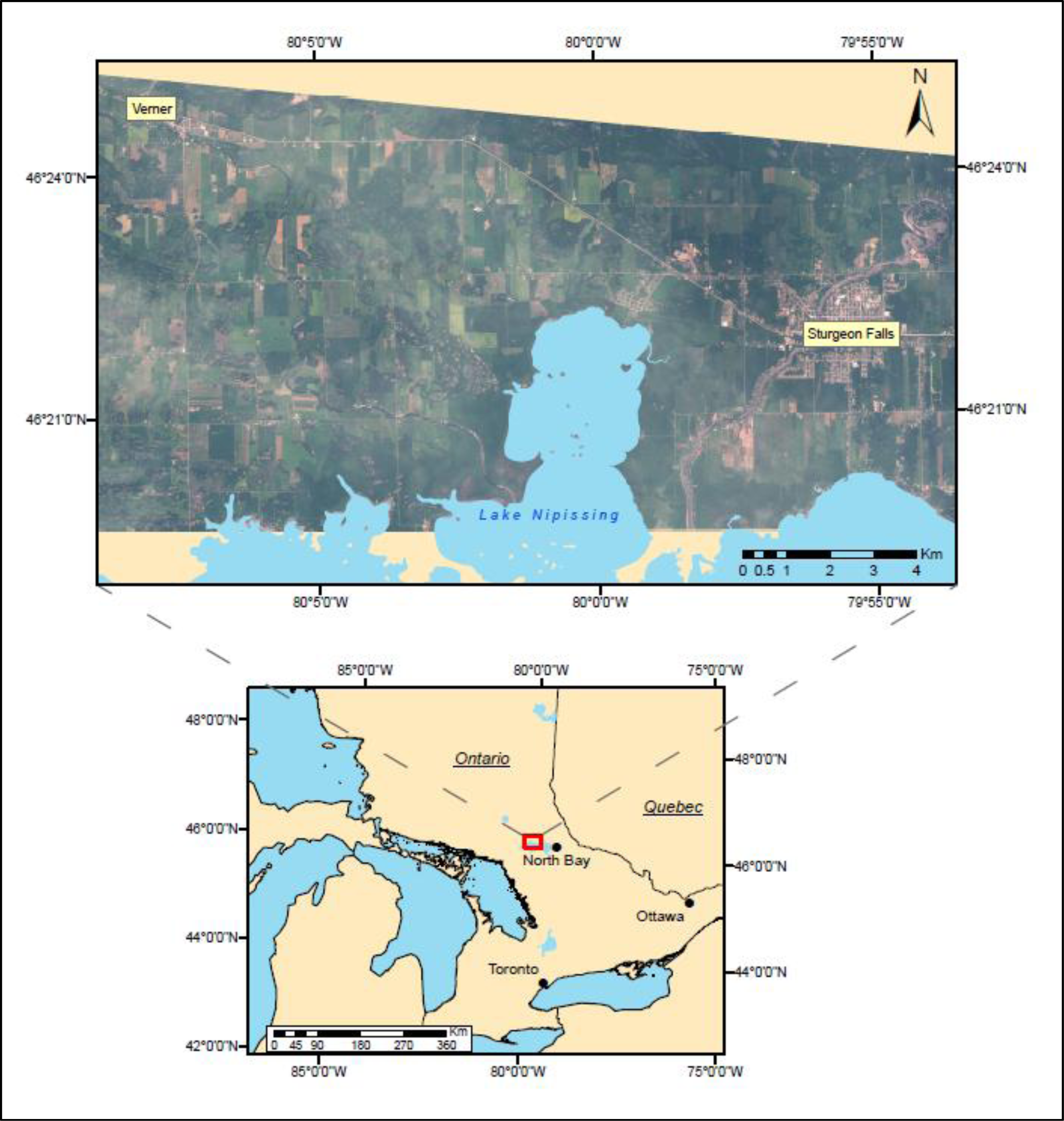
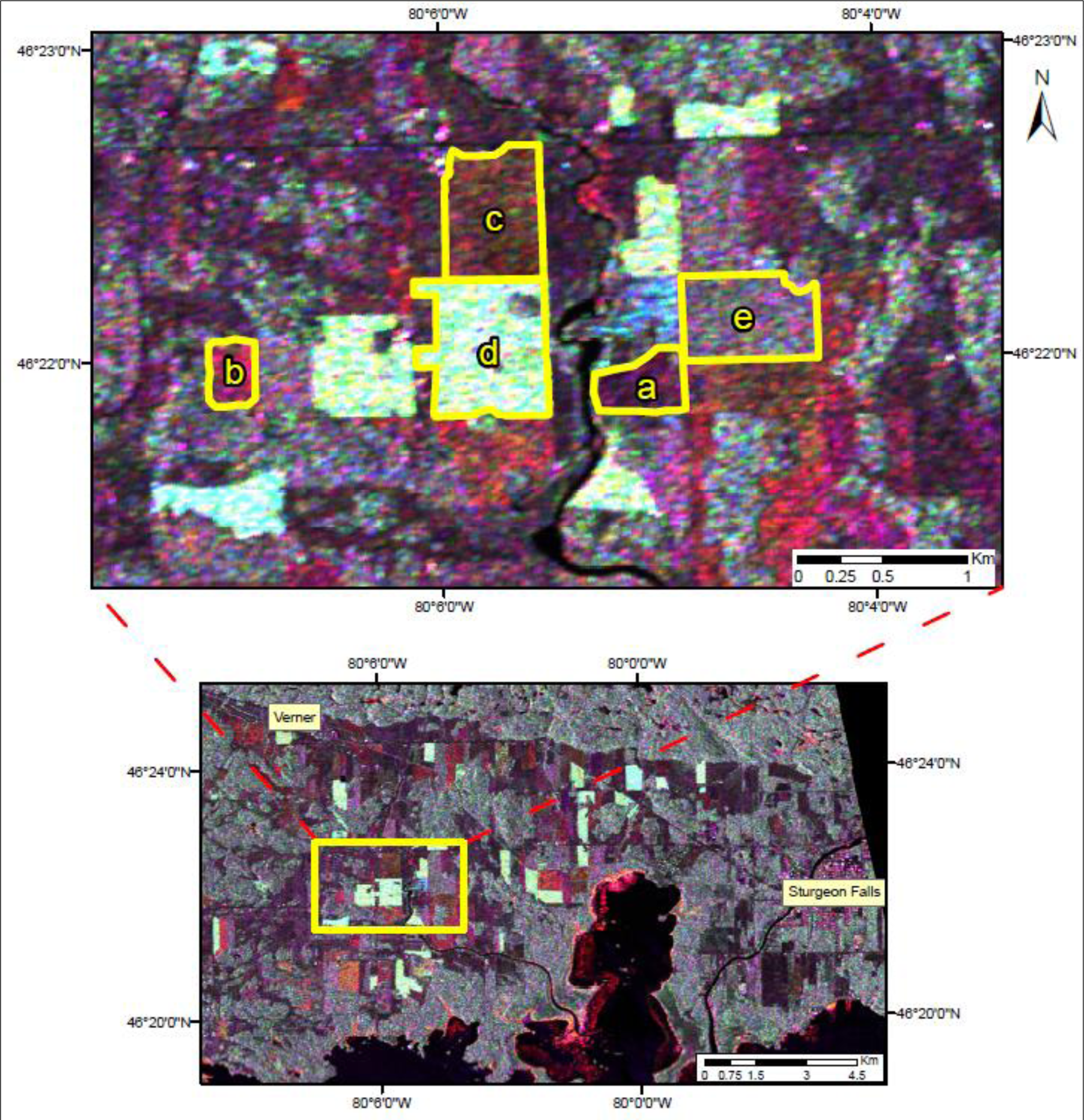
2. Study Area
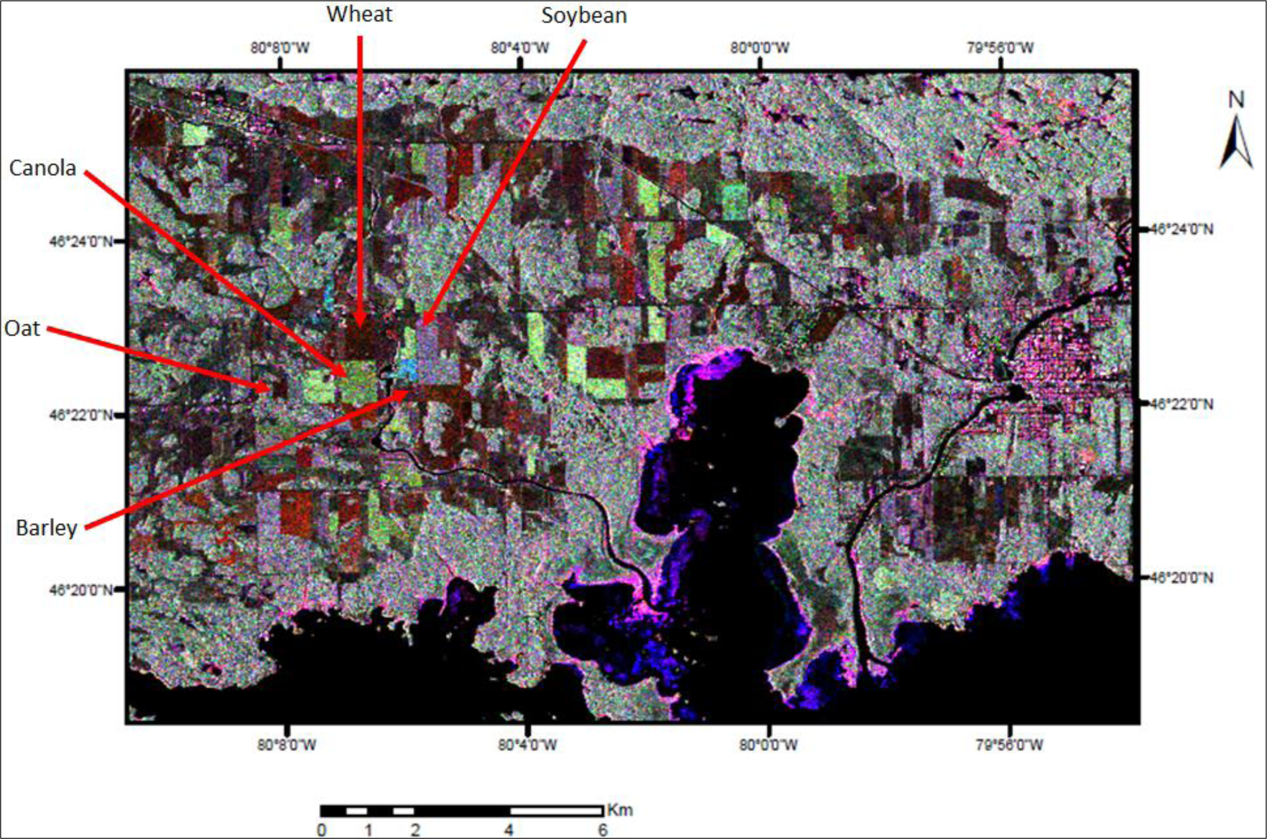
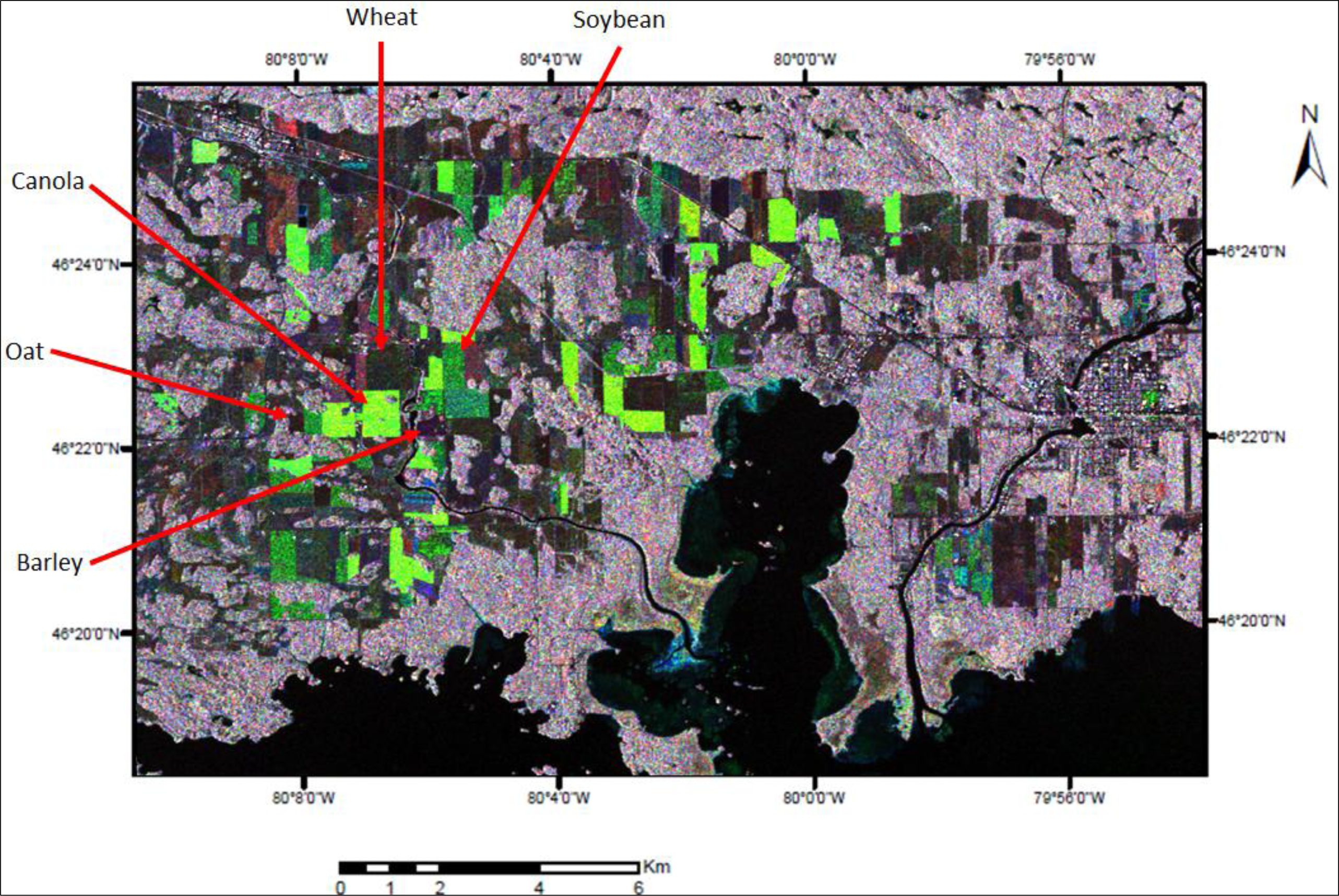
3. Crop Types
4. Methodology
4.1. Satellite Imagery
4.2. Field Data
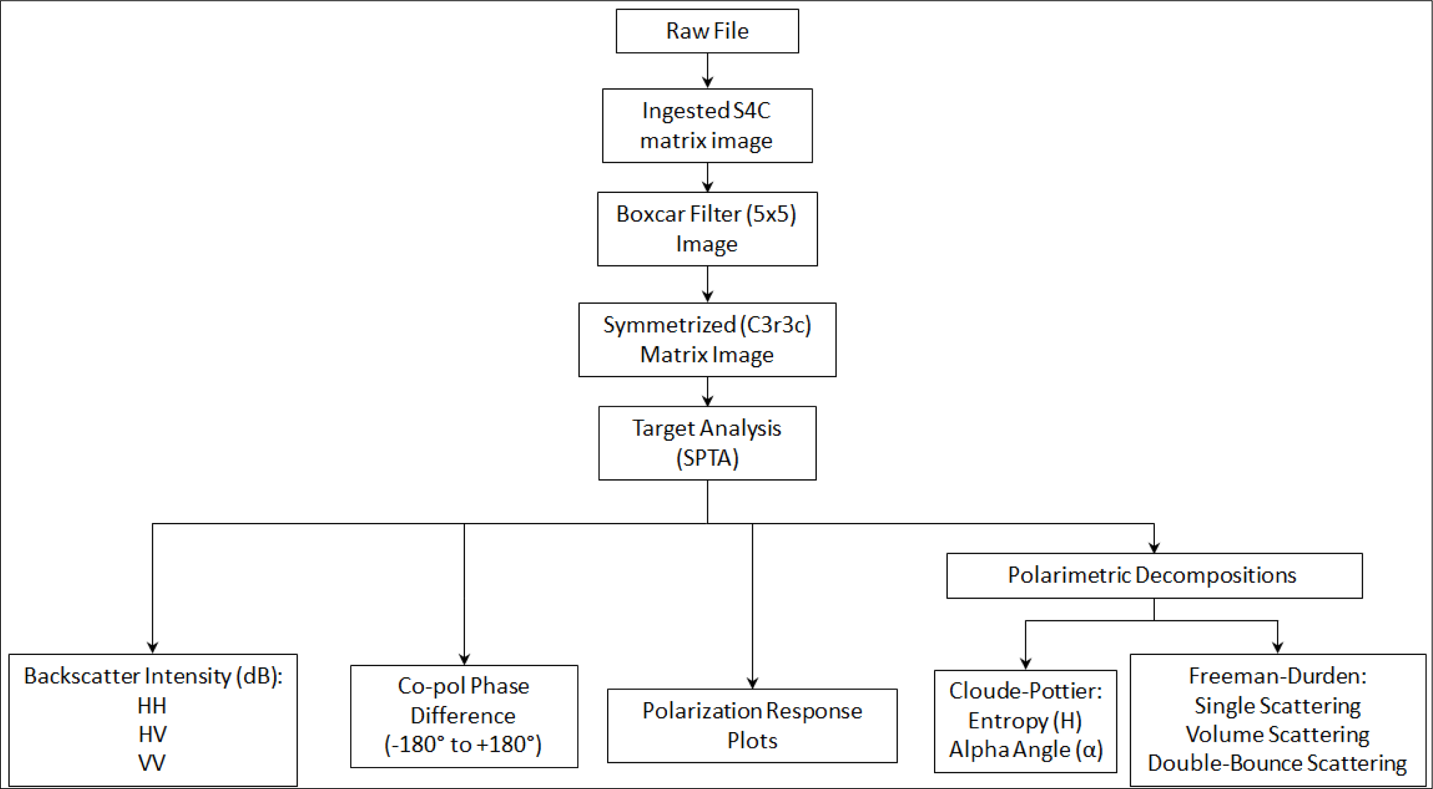
4.3. Data Processing
4.4. Data Extraction
5. Results and Discussion
5.1. Backscatter Intensity
5.2. Co-Polarized Phase Difference
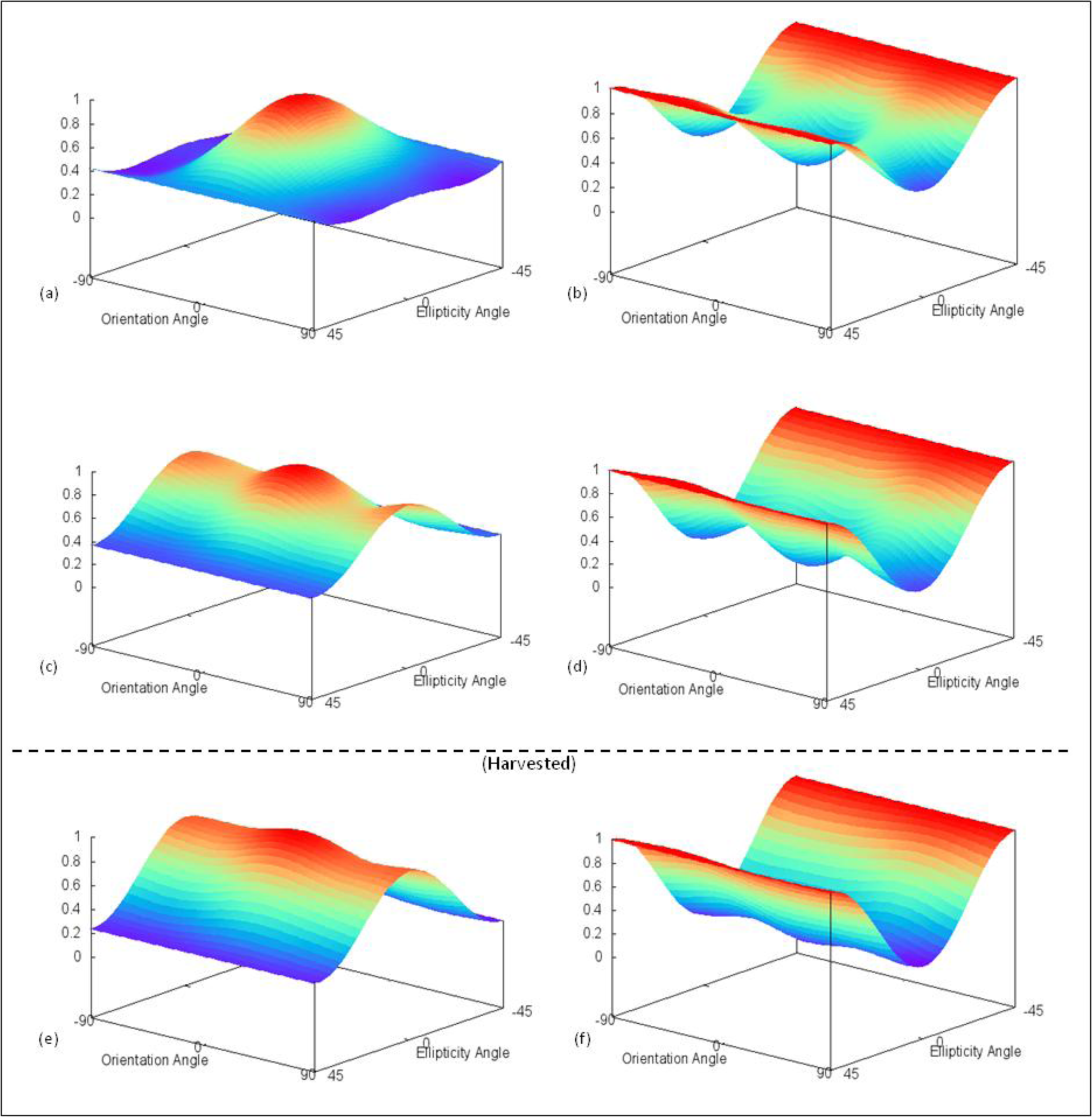
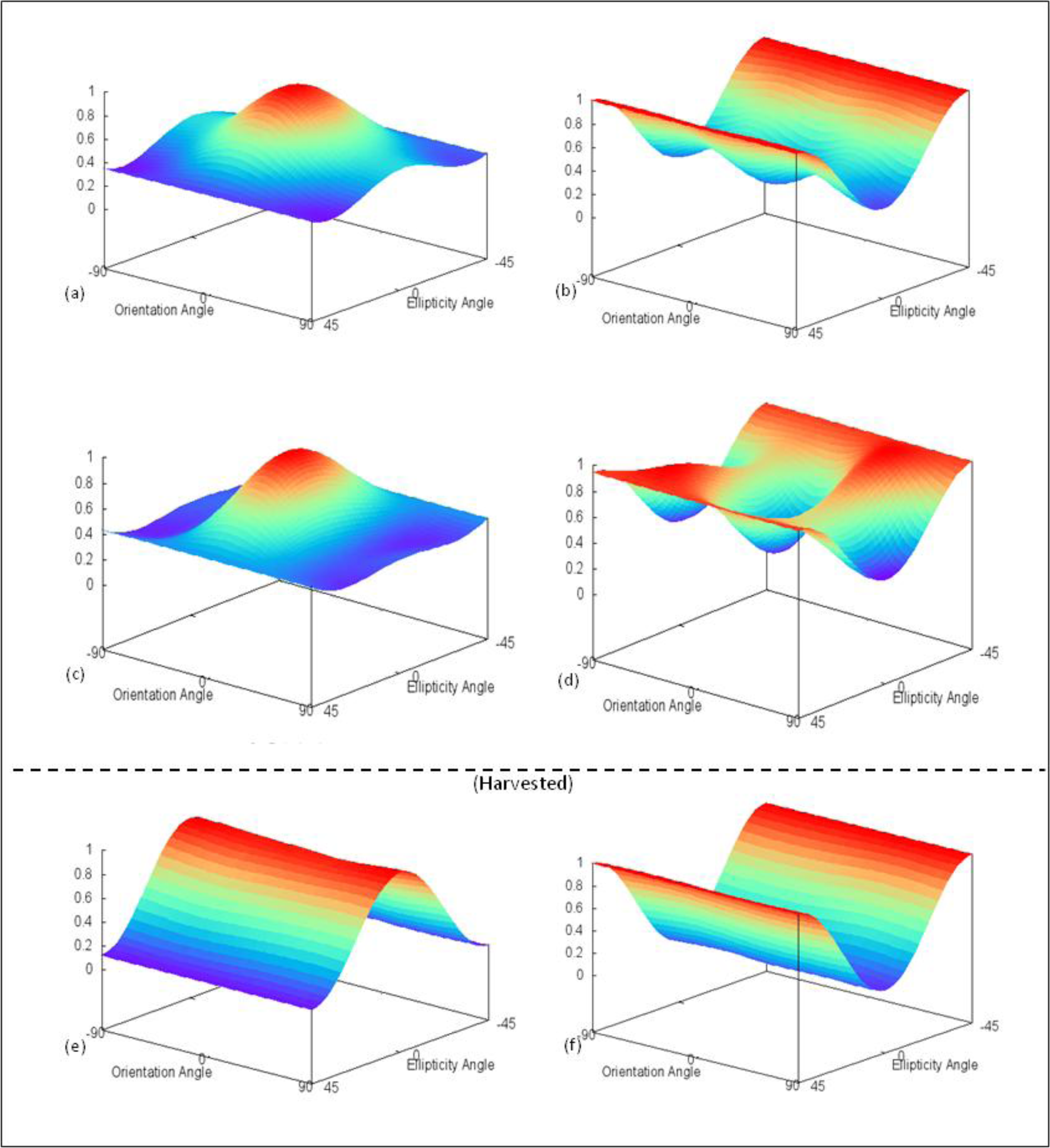
5.3. Polarimetric Response Plots and Decompositions
5.3.1. Barley
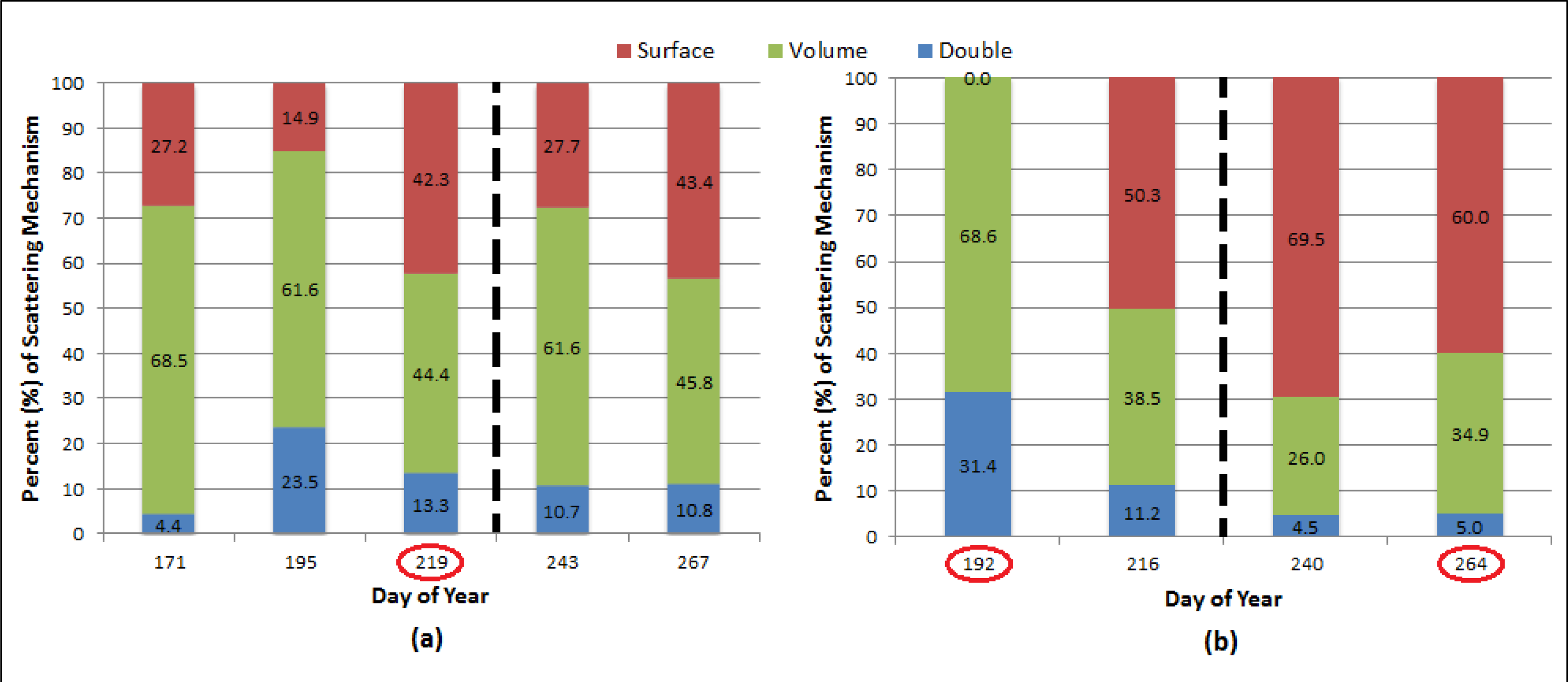
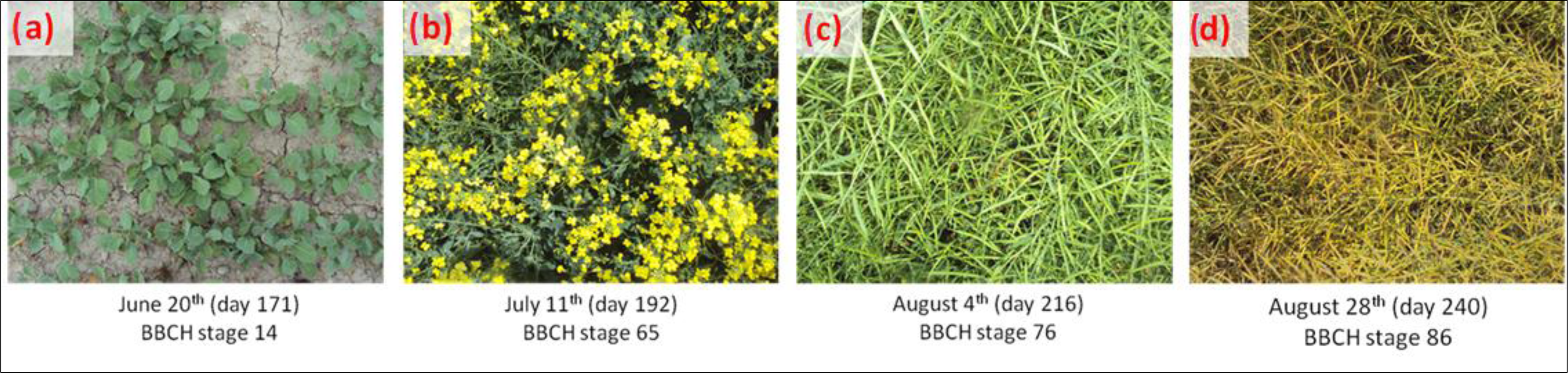
5.3.2. Canola
5.3.3. Oat
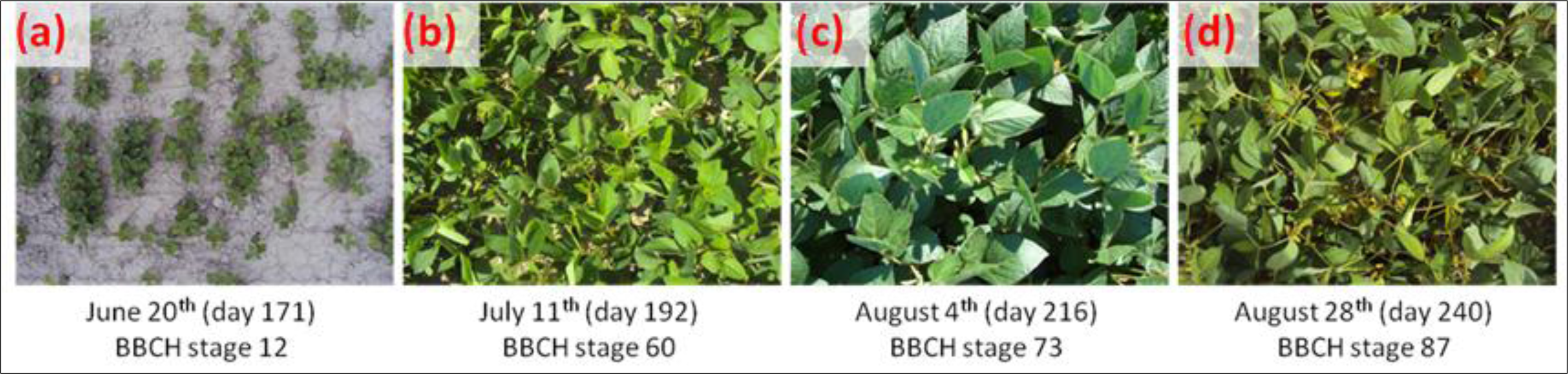
5.3.4. Soybean
5.3.5. Wheat
6. Conclusions
Supplementary Information
remotesensing-06-02343-s001.pdfAcknowledgments
Authors Contributions
Conflicts of Interest
References
- Kittson, K. An Overview of the Canadian Agriculture and Agri-Food System; Research and Analysis Directorate, Stategic Policy Branch, Agriculture and Agri-Food Canada: Ottawa, ON, Canada, 2013. [Google Scholar]
- Skriver, H.; Svendsen, M.T.; Thomsen, A.G. Multitemporal C- and L-band polarimetric signatures of crops. IEEE Trans. Geosci. Remote Sens 1999, 37, 2413–2429. [Google Scholar]
- McNairn, H.; Hochheim, K.; Rabe, N. Applying polarimetric radar imagery for mapping the productivity of wheat crops. Can. J. Remote Sens 2004, 30, 517–524. [Google Scholar]
- Soria-Ruiz, J.; McNairn, H.; Fernandez-Ordonez, Y.; Bugden-Storie, J. Corn Monitoring and Crop Yield Using Optical and RADARSAT-2 Images. Proceedings of the 2009 IEEE Geoscience and Remote Sensing Symposium (IGARSS), Barcelona, Spain, 23–28 July 2007.
- Wang, D.; Lin, H.; Chen, J.; Zhang, Y.; Zeng, Q. Application of multi-temporal ENVISAT ASAR data to agricultural area mapping in the Pearl River Delta. Int. J. Remote Sens 2010, 31, 1555–1572. [Google Scholar]
- Kim, Y.; Jackson, T.; Bindlish, R.; Lee, H.; Hong, S. Monitoring soybean growth using L-, C- and X-band scatterometer data. Int. J. Remote Sens 2013, 34, 4069–4082. [Google Scholar]
- Adams, J.R.; Rowlandson, T.L.; McKeown, S.J.; Berg, A.A.; McNairn, H.; Sweeny, S.J. Evaluating the Cloude-Pottier and Freeman-Durden scattering decompositions for distinguishing between unharvested and post-harvested agricultural fields. Can. J. Remote Sens 2013, 39, 1–10. [Google Scholar]
- Brisco, B.; Brown, R.J. Agricultural Applications with Radar. In Manual of Remote Sensing: Principles and Applications of Imaging Radar, 3rd ed; Henderson, F.M., Lewis, A.J., Eds.; John Wiley and Sons: Toronto, Canada, 1998; Volume 2, pp. 381–406. [Google Scholar]
- Kim, Y.; van Zyl, J.J. A time-series approach to estimate soil moisture using polarimetric radar data. IEEE Trans. Geosci. Remote Sens 2009, 47, 2519–2527. [Google Scholar]
- McNairn, H.; Duguay, C.; Brisco, B.; Pultz, T.J. The effect of soil and crop residue characteristics on polarimetric radar response. Remote Sens. Environ 2002, 80, 308–320. [Google Scholar]
- Ulaby, F.T.; Held, D.; Dobson, M.C.; McDonald, K.C.; Senior, T.B.A. Relating polarization phase difference of SAR signals to scene properties. IEEE Trans. Geosci. Remote Sens 1987, 25, 83–92. [Google Scholar]
- Shang, J.; McNairn, H.; Deschamps, J.; Jiao, X. In-season crop inventory using multi-angle and multi-pass RADARSAT-2 SAR data over the Canadian prairies. Proc. SPIE 2011. [Google Scholar] [CrossRef]
- Vaglio Laurin, G.; Del Frate, F.; Pasolli, L.; Notarnicola, C.; Guerriero, L.; Valentini, R. Discrimination of vegetation types in alpine sites with ALOS PALSAR-, RADARSAT-2- and lidar-derived information. Int. J. Remote Sens 2013, 34, 6898–6913. [Google Scholar]
- McNairn, H.; Shang, J.; Champagne, C.; Jiao, X. TERRASAR-X and RADARSAT-2 for Crop Classification and Acreage Estimation. Proceedings of the 2009 IEEE International Geoscience and Remote Sensing Symposium (IGARSS), Cape Town, South Africa, 12–17 July 2009.
- Liu, C.; Shang, J.; Vachon, P.W.; McNairn, H. Multiyear crop monitoring using polarimetric RADARSAT-2 data. IEEE Trans. Geosci. Remote Sens 2013, 51, 2227–2240. [Google Scholar]
- Cable, J.W.; Kovacs, J.M.; Shang, J.; Jiao, X. Multi-temporal polarimetric RADARSAT-2 for land cover monitoring in Northeastern Ontario, Canada. Remote Sens 2014. In press. [Google Scholar]
- Webber, L.R.; Hoffman, D.W. Origin, Classification and Use of Ontario Soils; Ontario Department of Agriculture and Food: Toronto, ON, Canada, 1970; p. 58. [Google Scholar]
- Baldwin, D.J.B.; Desloges, J.R.; Band, L.E. Physical Geography of Ontario. In Ecology of a Managed Terrestrial Landscape: Patterns and Processes of Forest Landscapes in Ontario; Perera, A.H., Euler, D.E., Thompson, I.D., Eds.; University of British Columbia Press: Vancouver, BC, Canada, 2000; pp. 141–162. [Google Scholar]
- The Corporation of the Municipality of West Nipissing. Agriculture in West Nipissing. Available online: http://www.westnipissingouest.ca/agriculture.html (accessed on 26 April 2012).
- Decagon Devices. AccuPAR LP-80. Available online: http://www.decagon.com/products/environmental-instruments/ceptometer-par-lai-instruments-2/accupar-lp-80/ (accessed on 15 June 2013).
- Jiao, X.; McNairn, H.; Shang, J.; Pattey, E.; Liu, J.; Champagne, C. The sensitivity of RADARSAT-2 polarimetric SAR data to corn and soybean leaf area index (LAI). Can. J. Remote Sens 2011, 37, 69–81. [Google Scholar]
- Li, K.; Brisco, B.; Yun, S. Polarimetric decomposition with RADARSAT-2 for rice mapping and monitoring. Can. J. Remote Sens 2012, 38, 169–179. [Google Scholar]
- Lee, J.S.; Pottier, E. Polarimetric Radar Imaging; CRC Press: Boca Raton, FL, USA, 2009; p. 398. [Google Scholar]
- Boerner, W.M.; Mott, H.; Luneburg, E.; Livingstone, C.; Brisco, B.; Brown, R.J.; Patterson, J.S. Polarimetry in Radar Remote Sensing: Basic and Applied Concepts. In Manual of Remote Sensing: Principles and Applications of Imaging Radar, 3rd ed; Henderson, F.M., Lewis, A.J., Eds.; John Wiley and Sons: Toronto, ON, Canada, 1998; Volume 2, pp. 271–356. [Google Scholar]
- Van Zyl, J.J.; Zebker, H.A.; Elachi, C. Imaging radar polarization signatures: Theory and observations. Radio Sci 1987, 22, 529–543. [Google Scholar]
- Cloude, S.R.; Pottier, E. An entropy classificationscheme for land applications of polarimetric SAR data. IEEE Trans. Geosci. Remote Sens 1997, 35, 68–78. [Google Scholar]
- Freeman, A.; Durden, S.L. A three-component scattering model for polarimetric SAR data. IEEE Trans. Geosci. Remote Sens 1998, 36, 963–973. [Google Scholar]
- Van Zyl, J.J.; Zebker, H.A. Imaging Radar Polarimetry. In Progress in Electromagnetics Research 3: Polarimetric Remote Sensing; Kong, J.A., Ed.; Elsevier: New York, NY, USA, 1990; pp. 277–326. [Google Scholar]
- Baghdadi, N.; Cresson, R.; Pottier, E.; Aubert, M.; Zribi, M.; Jacome, A.; Benabdallah, S. A potential use for the C-band polarimetric SAR parameters to characterize the soil surface over bare agricultural fields. IEEE Trans. Geosci. Remote Sens 2012, 50, 3844–3858. [Google Scholar]
- McNairn, H.; Shang, J.; Jiao, X.; Champagne, C. The contribution of ALOS PALSAR multipolarization and polarimetric data to crop classification. IEEE Trans. Geosci. Remote Sens 2009, 47, 3981–3992. [Google Scholar]


| Acquisition Date | Day of Year | Polarization (Beam Mode) | Pixel Size (m) | Incidence Angle (°) |
|---|---|---|---|---|
| 20 June 2011 | 171 | Polarimetric (FQ21) | 10 | 41 |
| 11 July 2011 | 192 | Polarimetric (FQ7) | 10 | 26 |
| 14 July 2011 | 195 | Polarimetric (FQ21) | 10 | 41 |
| 4 August 2011 | 216 | Polarimetric (FQ7) | 10 | 26 |
| 7 August 2011 | 219 | Polarimetric (FQ21) | 10 | 41 |
| 28 August 2011 | 240 | Polarimetric (FQ7) | 10 | 26 |
| 31 August 2011 | 243 | Polarimetric (FQ21) | 10 | 41 |
| 21 September 2011 | 264 | Polarimetric (FQ7) | 10 | 26 |
| 24 September 2011 | 267 | Polarimetric (FQ21) | 10 | 41 |
| Week of Acquisition (Day of Year) | ||||||
|---|---|---|---|---|---|---|
| Crop | Parameter | 20 June (171) | 11 July (192) | 4 August (216) | 28 August (240) * | 21 September (264) |
| Soybean | Avg. BBCH growth stage | 12 | 60 | 73 | 87 | |
| Avg. Height (cm) | 10 | 56 | 92 | 90 | ||
| Avg. LAI | N/A | 3.12 | 4.54 | 3.93 | ||
| Avg. Soil Moisture (%) | N/A | 18.5 | 12.4 | 11.3 | 21.8 | |
| Canola | Avg. BBCH growth stage | 14 | 65 | 76 | 86 | |
| Avg. Height (cm) | 19 | 137 | 151 | 145 | ||
| Avg. LAI | N/A | 5.14 | 4.59 | 3.33 | ||
| Avg. Soil Moisture (%) | N/A | 16.7 | 14.0 | 13.5 | 21.9 | |
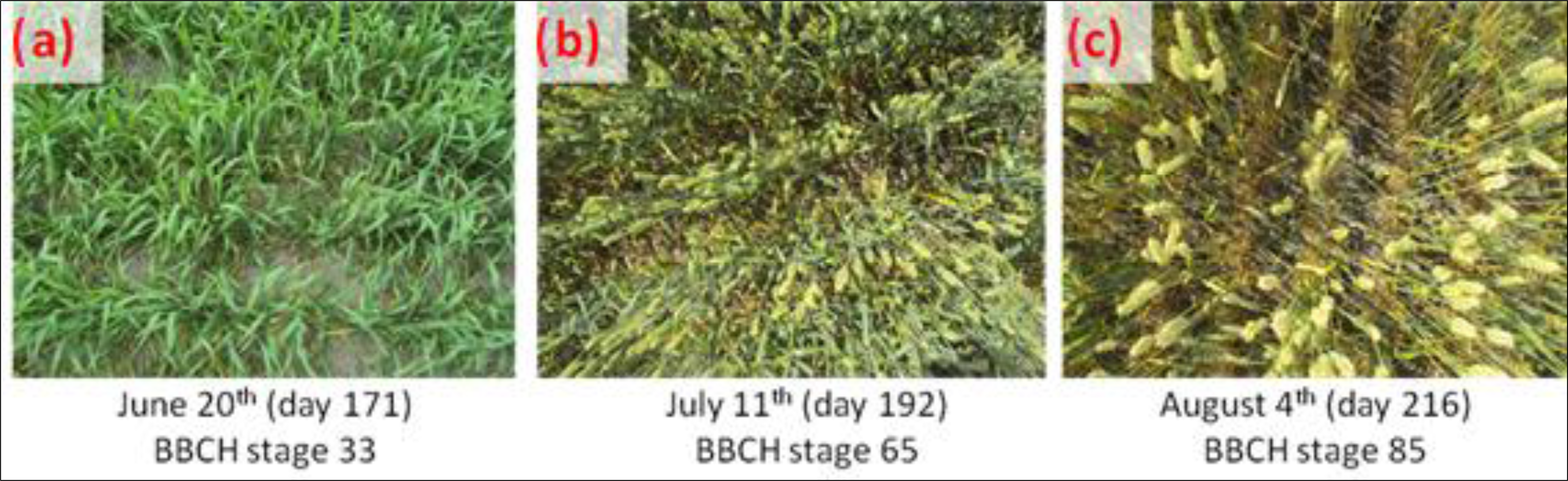
| Wheat | Avg. BBCH growth stage | 33 | 65 | 85 | ||
| Avg. Height (cm) | 49 | 89 | 90 | |||
| Avg. LAI | N/A | 3.03 | 2.16 | |||
| Avg. Soil Moisture (%) | N/A | 14.4 | 10.8 | 11.6 | 18.7 | |
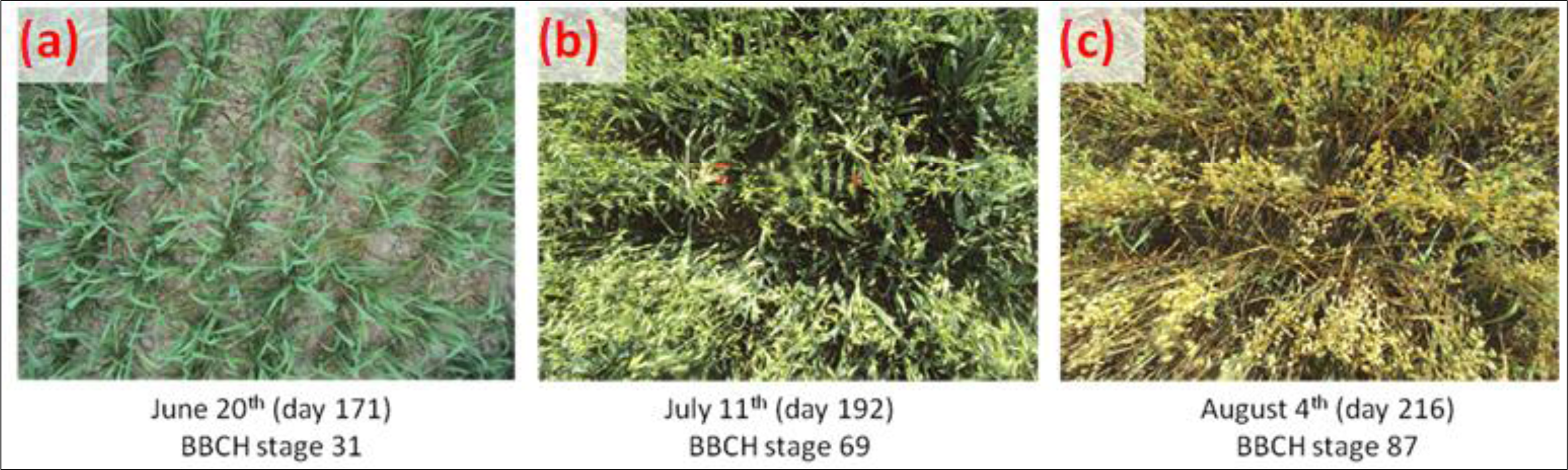
| Oat | Avg. BBCH growth stage | 31 | 69 | 87 | ||
| Avg. Height (cm) | 41 | 105 | 106 | |||
| Avg. LAI | N/A | 3.33 | 2.33 | |||
| Avg. Soil Moisture (%) | N/A | 15.4 | 11.9 | 12.7 | 19.5 | |
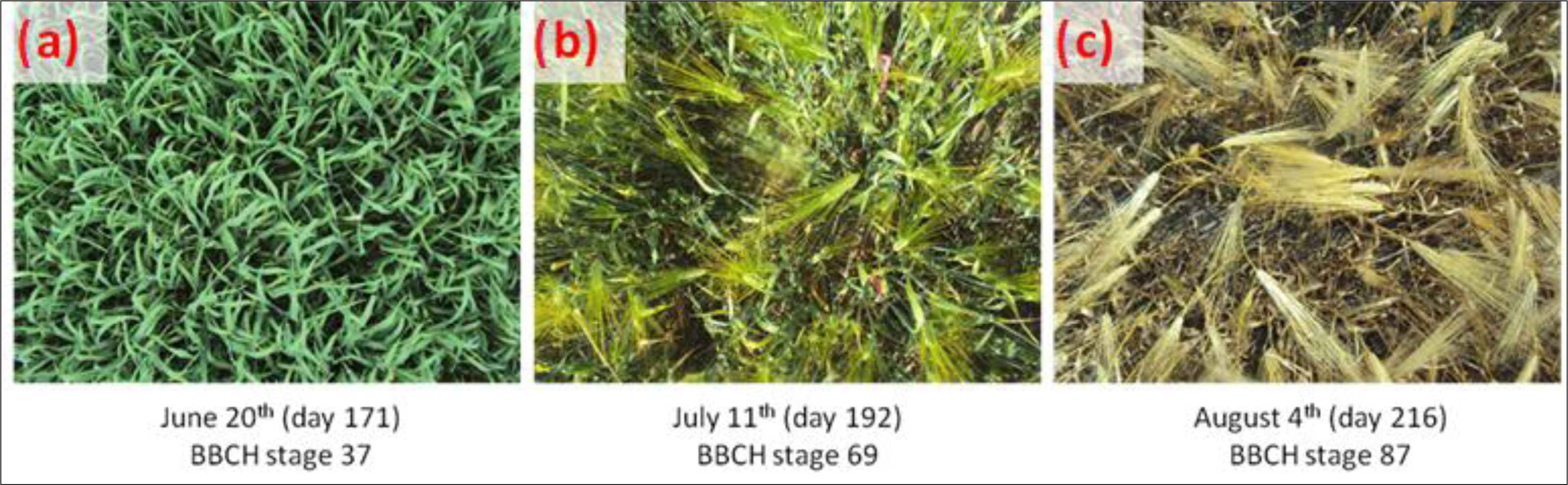
| Barley | Avg. BBCH growth stage | 37 | 69 | 87 | ||
| Avg. Height (cm) | 52 | 115 | 107 | |||
| Avg. LAI | N/A | 2.96 | 1.96 | |||
| Avg. Soil Moisture (%) | N/A | 15.1 | 11.4 | 11.7 | 18.2 | |
© 2014 by the authors; licensee MDPI, Basel, Switzerland This article is an open access article distributed under the terms and conditions of the Creative Commons Attribution license (http://creativecommons.org/licenses/by/3.0/).
Share and Cite
Cable, J.W.; Kovacs, J.M.; Jiao, X.; Shang, J. Agricultural Monitoring in Northeastern Ontario, Canada, Using Multi-Temporal Polarimetric RADARSAT-2 Data. Remote Sens. 2014, 6, 2343-2371. https://doi.org/10.3390/rs6032343
Cable JW, Kovacs JM, Jiao X, Shang J. Agricultural Monitoring in Northeastern Ontario, Canada, Using Multi-Temporal Polarimetric RADARSAT-2 Data. Remote Sensing. 2014; 6(3):2343-2371. https://doi.org/10.3390/rs6032343
Chicago/Turabian StyleCable, Jeffrey W., John M. Kovacs, Xianfeng Jiao, and Jiali Shang. 2014. "Agricultural Monitoring in Northeastern Ontario, Canada, Using Multi-Temporal Polarimetric RADARSAT-2 Data" Remote Sensing 6, no. 3: 2343-2371. https://doi.org/10.3390/rs6032343