A Novel Land Cover Classification Map Based on a MODIS Time-Series in Xinjiang, China


Abstract
:1. Introduction
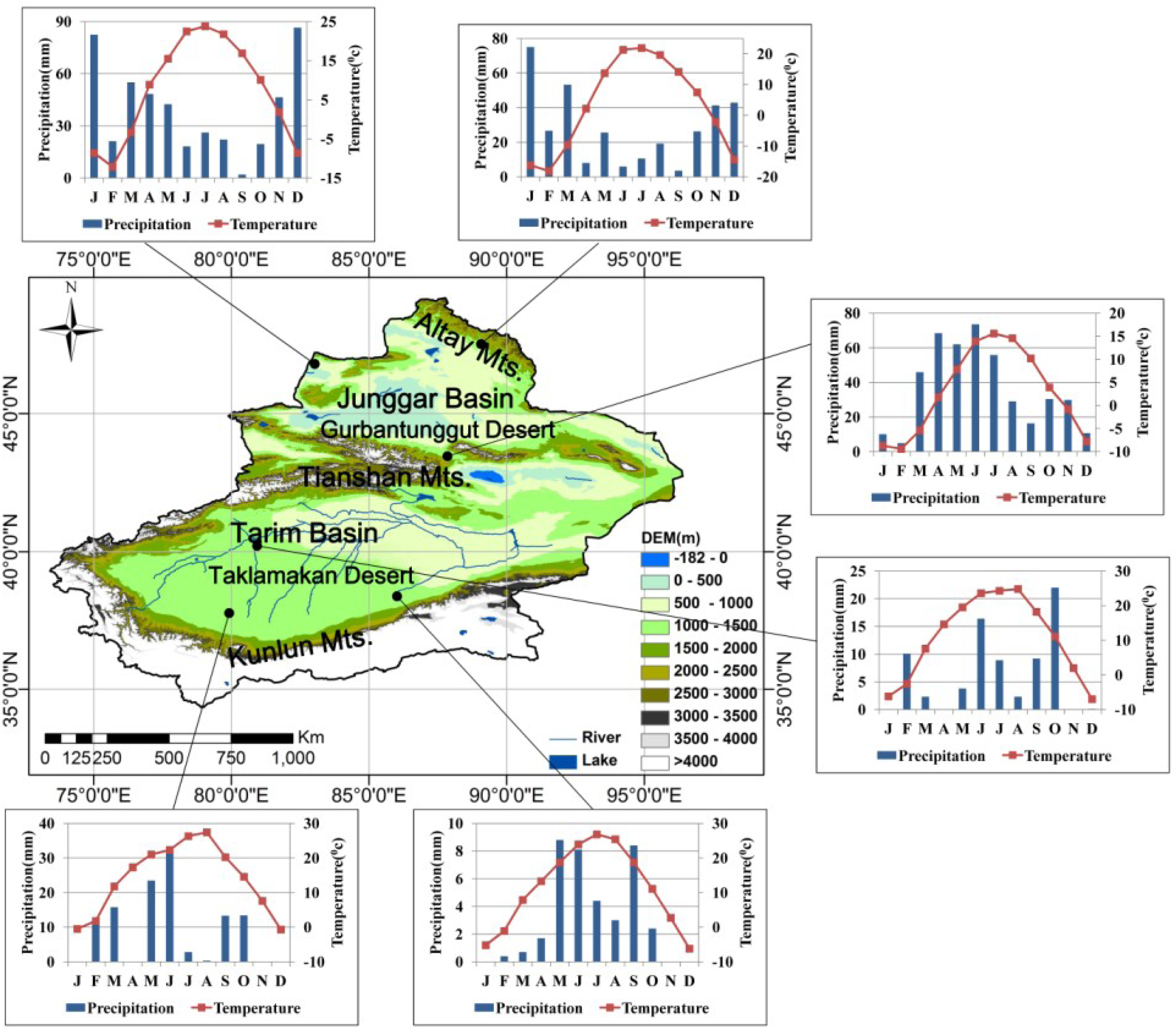
2. Study Area
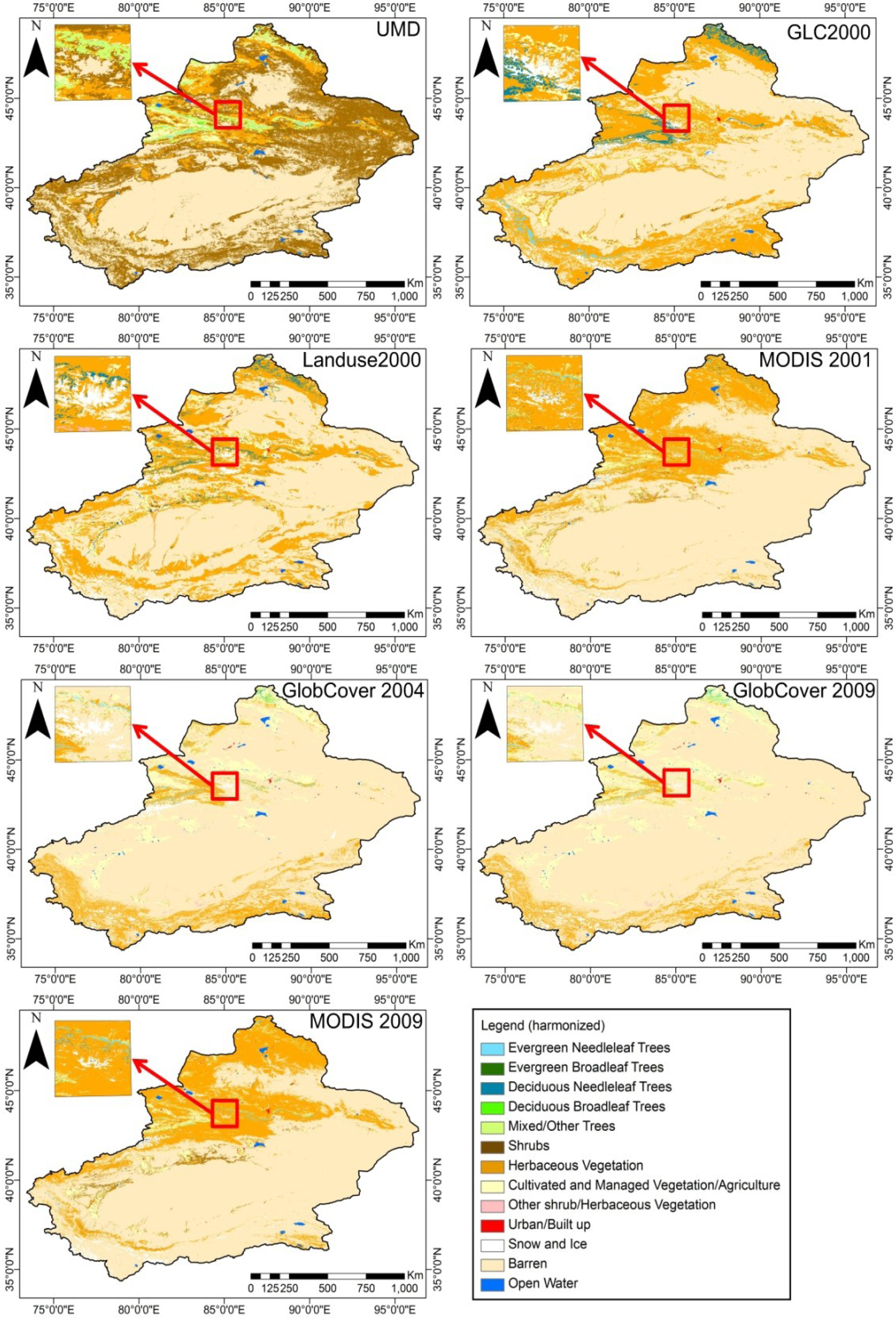
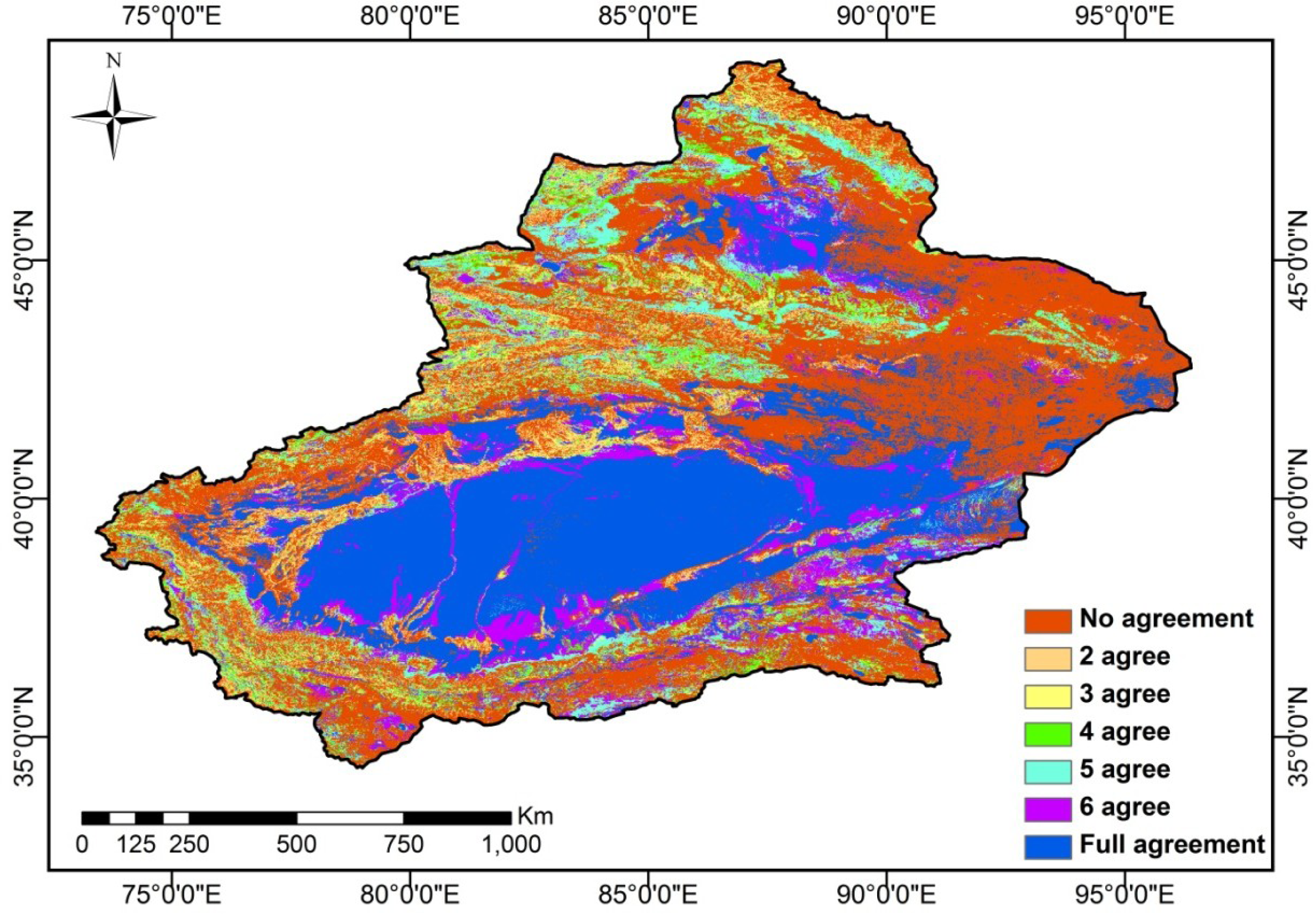
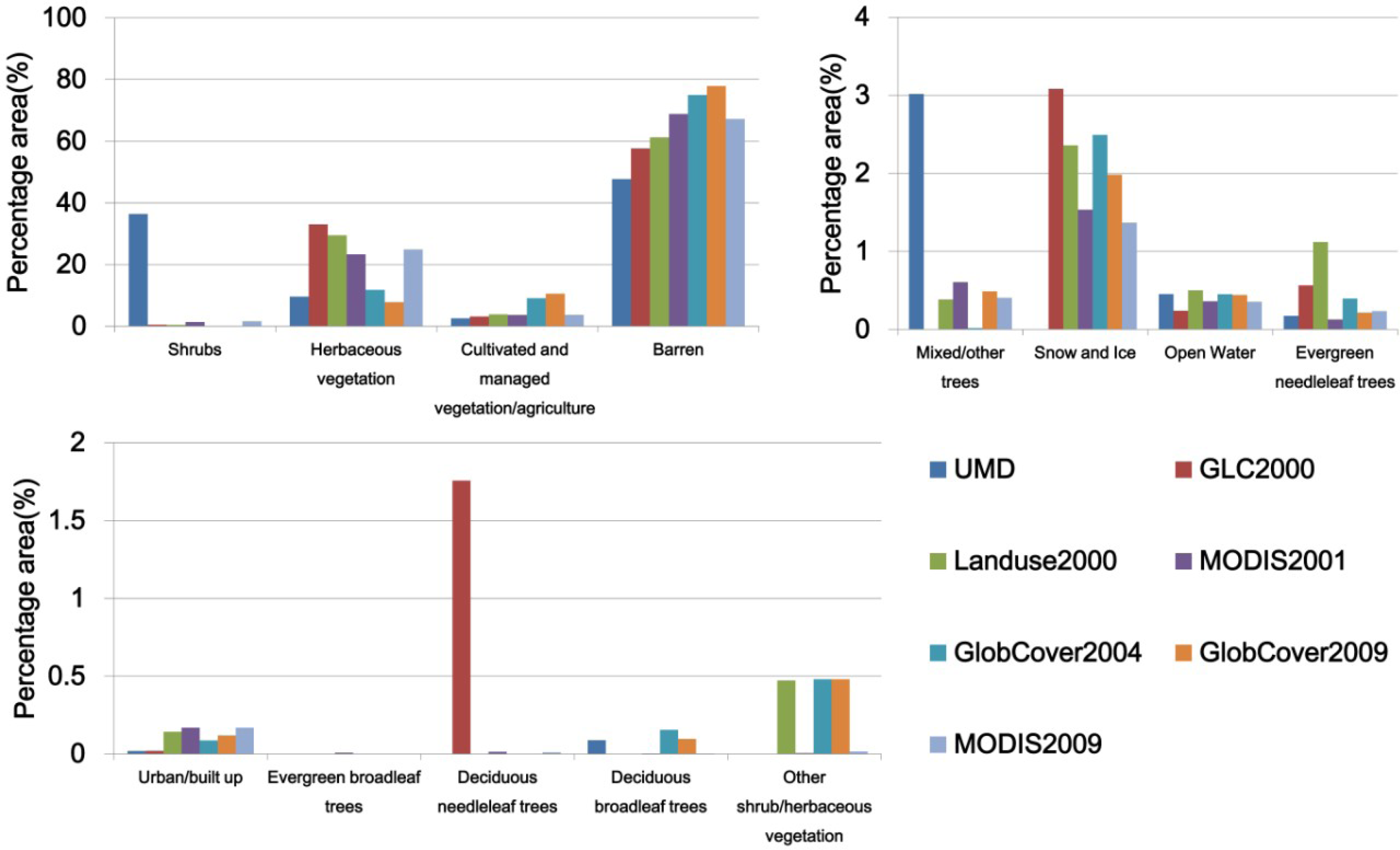
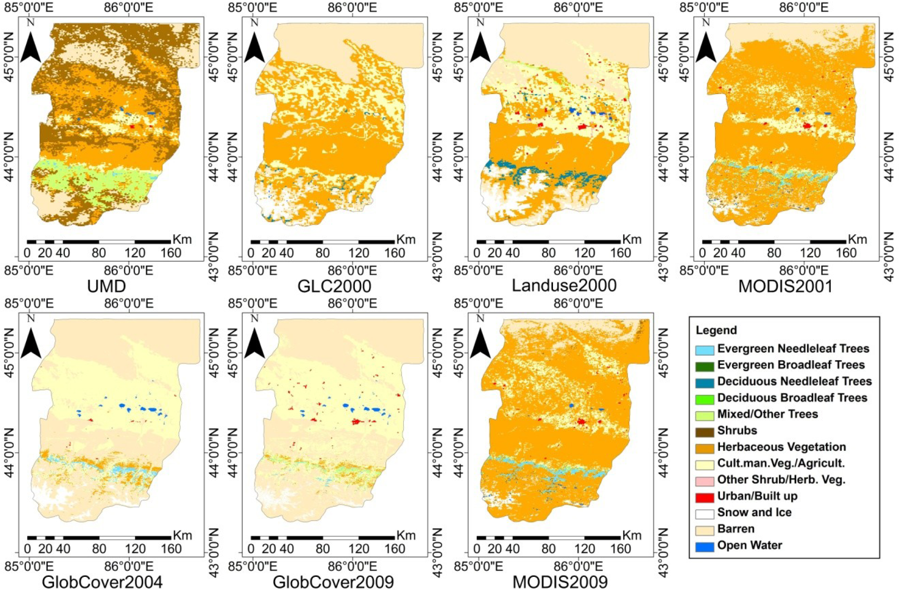
3. The Requirement for a Novel Land Cover Product over the XUAR
- No agreement—pixels containing different LCCS classes in each dataset;
- Level 2 to level 6 agreement—pixels in which two to six of the seven datasets are in agreement, respectively;
- Full agreement—pixels in which all of the seven datasets were in agreement.
4. Classification Approach
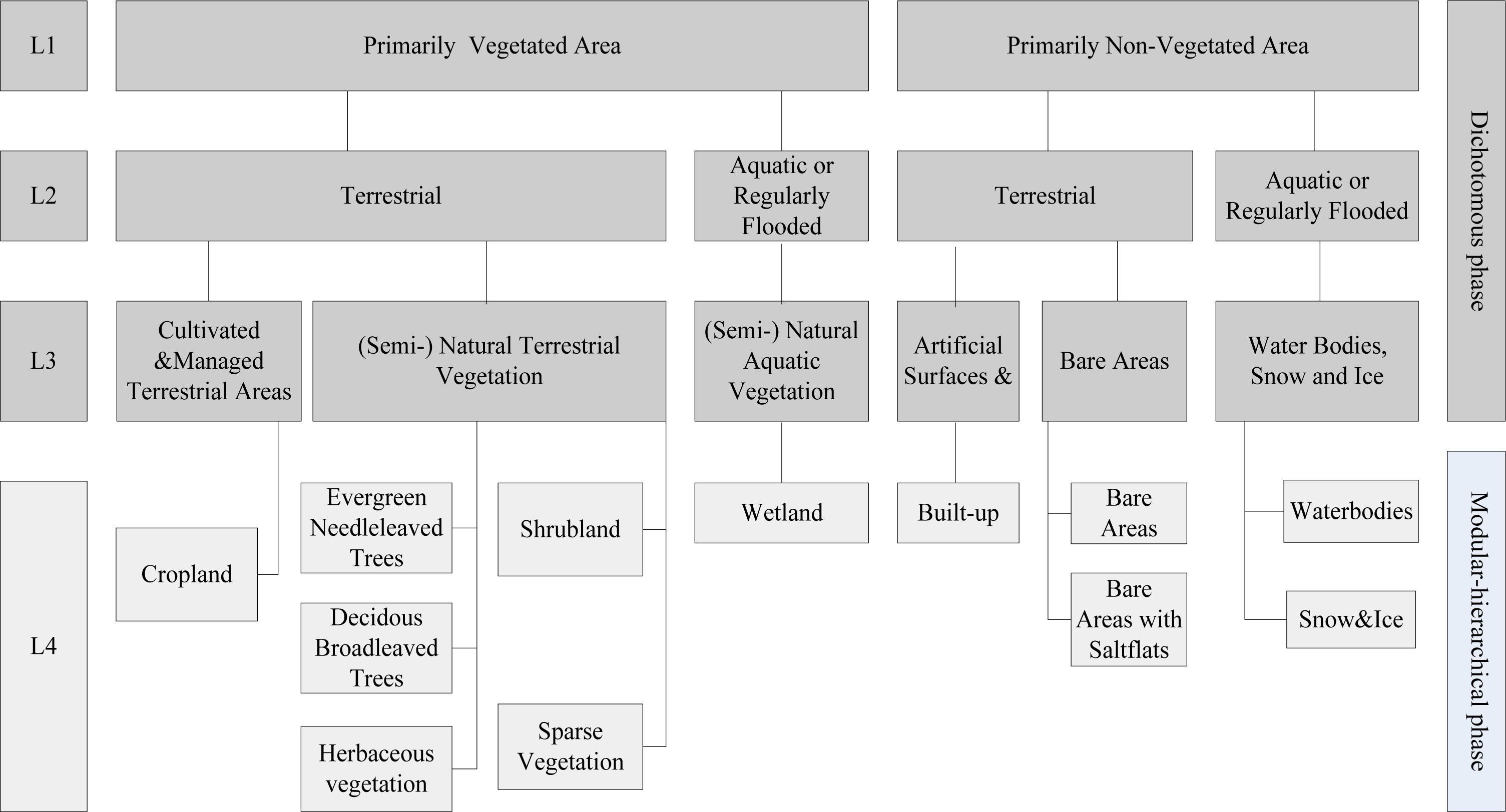
4.1. Classification Scheme
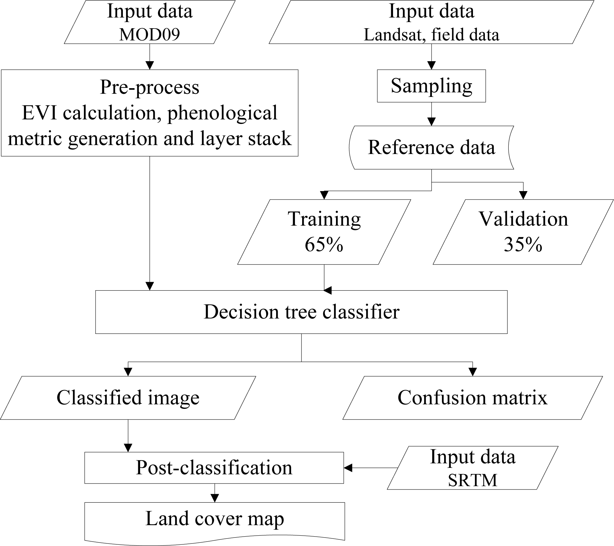
4.2. Methodology
4.2.1. C5.0 Based Decision Tree Classification
4.2.2. Input Data
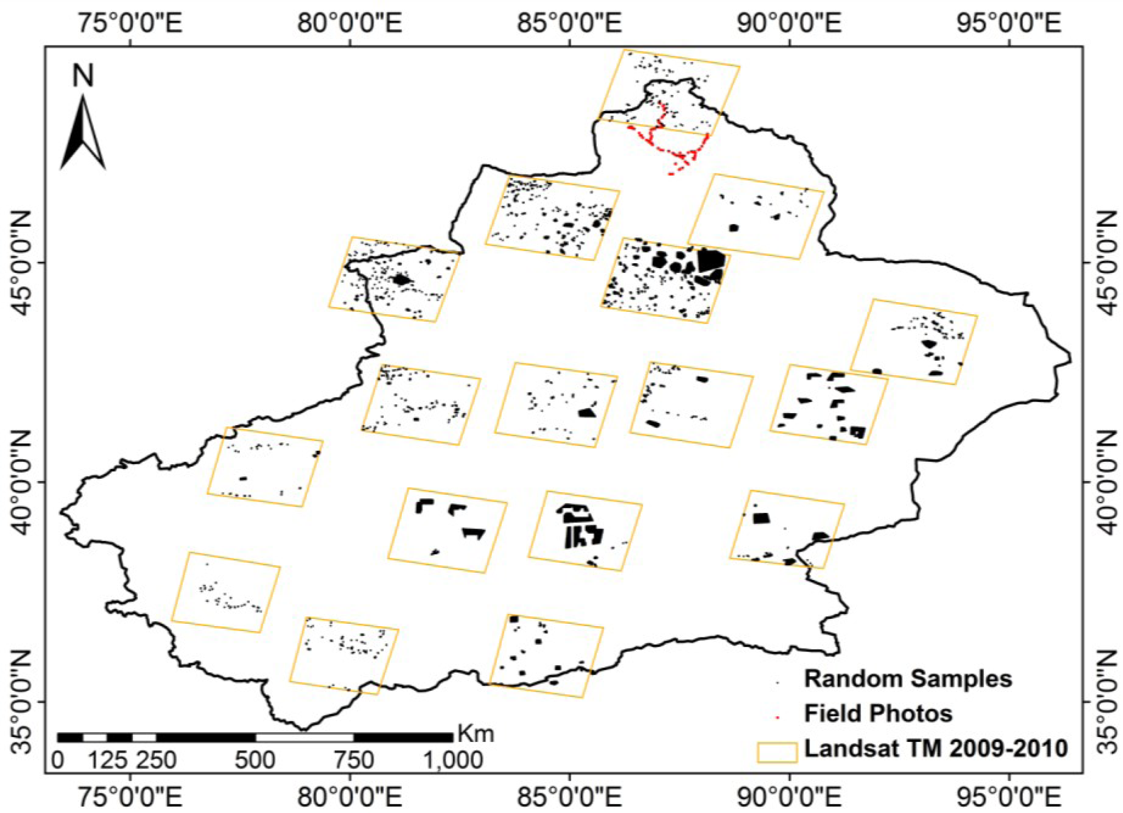
4.2.3. Training and Validation Data Collection
4.2.4. Post Classification
5. Results
5.1. Land Cover Classification Map
5.2. Accuracy Assessment
6. Discussion
7. Conclusions
Acknowledgments
Author Contributions
Conflicts of Interest
References
- Di Gregorio, A. Land Cover Classification System––Classification Concepts and User Manual for Software Version 2; Food and Agriculture Organization of the United Nations: Rome, Italy, 2005. [Google Scholar]
- Meyer, W.B.; Turner, B.L., II. Human population growth and global land use/land cover change. Ann. Rev. Ecol. Syst 1992, 23, 39–61. [Google Scholar]
- Foley, J.A.; DeFries, R.; Asner, G.P.; Barford, C.; Bonan, G.; Carpenter, S.R.; Chapin, F.S.; Coe, M.T.; Daily, G.C.; Gibbs, H.K.; et al. Global consequences of land use. Science 2005, 309, 570–574. [Google Scholar]
- Lubchenco, J. Entering the century of the environment: A new social contract for science. Science 1998, 279, 491–497. [Google Scholar]
- DeFries, R.; Hansen, M.; Townshend, J. Global discrimination of land cover types from metrics derived from AVHRR pathfinder data. Remote Sens. Environ 1995, 54, 209–222. [Google Scholar]
- Defries, R.S.; Townshend, J.R.G. NDVI-derived land-cover classifications at a global-scale. Int. J. Remote Sens 1994, 15, 3567–3586. [Google Scholar]
- Bartholome, E.; Belward, A.S. GLC2000: A new approach to global land cover mapping from Earth observation data. Int. J. Remote Sens 2005, 26, 1959–1977. [Google Scholar]
- Friedl, M.A.; Sulla-Menashe, D.; Tan, B.; Schneider, A.; Ramankutty, N.; Sibley, A.; Huang, X. MODIS Collection 5 global land cover: Algorithm refinements and characterization of new datasets. Remote Sens. Environ 2010, 114, 168–182. [Google Scholar]
- Arino, O.; Bicheron, P.; Achard, F.; Latham, J.; Witt, R.; Weber, J.L. GLOBCOVER—The Most Detailed Portrait of Earth. In ESA Bulletin Nr, 136; ESA Bulletin-European Space Agency: Rome, Italy, 2008; Volume 136, pp. 24–31. [Google Scholar]
- Verburg, P.H.; Neumann, K.; Nol, L. Challenges in using land use and land cover data for global studies. Glob. Chang. Biol 2011, 17, 974–989. [Google Scholar]
- Herold, M.; Mayaux, P.; Woodcock, C.E.; Baccini, A.; Schmullius, C. Some challenges in global land cover mapping: An assessment of agreement and accuracy in existing 1 Km datasets. Remote Sens. Environ 2008, 112, 2538–2556. [Google Scholar]
- Jung, M.; Henkel, K.; Herold, M.; Churkina, G. Exploiting synergies of global land cover products for carbon cycle modeling. Remote Sens. Environ 2006, 101, 534–553. [Google Scholar]
- Chandra, G.; Zhu, Z.; Reed, B. A comparative analysis of the global land cover 2000 and MODIS land cover data sets. Remote Sens. Environ 2005, 94, 123–132. [Google Scholar]
- Ran, Y.; Li, X.; Lu, L. Evaluation of four remote sensing based land cover products over China. Int. J. Remote Sens 2010, 31, 391–401. [Google Scholar]
- Vuolo, F.; Atzberger, C. Exploiting the classification performance of support vector machines with Multi-Temporal Moderate-Resolution Imaging Spectroradiometer (MODIS) data in areas of agreement and disagreement of existing land cover products. Remote Sens 2012, 4, 3143–3167. [Google Scholar]
- Kuenzer, C.; Leinenkugel, P.; Vollmuth, M.; Dech, S. Comparing global land cover products: An investigation for the trans-boundary Mekong basin. Int. J. Remote Sens 2014, in press. [Google Scholar]
- Pérez-Hoyos, A.; García-Haro, F.J.; San-Miguel-Ayanz, J. Conventional and fuzzy comparisons of large scale land cover products: Application to CORINE, GLC2000, MODIS and GlobCover in Europe. ISPRS J. Photogramm. Remote Sens 2012, 74, 185–201. [Google Scholar]
- Song, X.-P.; Huang, C.; Feng, M.; Sexton, J.O.; Channan, S.; Townshend, J.R. Integrating global land cover products for improved forest cover characterization: An application in North America. Int. J. Digit. Earth 2013. [Google Scholar] [CrossRef]
- Wang, T.; Yan, C.Z.; Song, X.; Xie, J.L. Monitoring recent trends in the area of aeolian desertified land using Landsat images in China’s Xinjiang region. ISPRS J. Photogramm. Remote Sens 2012, 68, 184–190. [Google Scholar]
- Cheng, W.; Zhou, C.; Liu, H.; Zhang, Y.; Jiang, Y.; Zhang, Y.; Yao, Y. The oasis expansion and eco-environment change over the last 50 years in Manas River Valley, Xinjiang. Sci. China Ser. D 2006, 49, 163–175. [Google Scholar]
- Yan, C.Z.; Wang, T.; Han, Z.W.; Qie, Y.F. Surveying sandy deserts and desertified lands in north-western China by remote sensing. Int. J. Remote Sens 2007, 28, 3603–3618. [Google Scholar]
- Buhe, A.; Tsuchiya, K.; Kaneko, M.; Ohtaishi, N.; Halik, M. Land cover of oases and forest in XinJiang, China retrieved from ASTER data. Adv. Space Res 2007, 39, 39–45. [Google Scholar]
- Huth, J.; Kuenzer, C.; Wehrmann, T.; Gebhardt, S.; Tuan, V.Q.; Dech, S. Land cover and land use classification with TWOPAC: Towards automated processing for pixel- and object-based image classification. Remote Sens 2012, 4, 2530–2553. [Google Scholar]
- Hansen, M.C.; Reed, B. A comparison of the IGBP DISCover and university of Maryland 1 Km global land cover products. Int. J. Remote Sens 2000, 21, 1365–1373. [Google Scholar]
- Fritz, S.; Bartholomé, E.; Belward, A.; Hartley, A.; Stibig, H.J.; Eva, H.; Mayaux, P.; Bartalev, S.; Latifovic, R.; Kolmert, S.; et al. Harmonization, Mosaicing and Production of the Global Land Cover 2000 Database (Beta Version); European Commission, Joint Research Centre: Ispra, Italy, 2003; p. 41. [Google Scholar]
- Mayaux, P.; Eva, H.; Gallego, J.; Strahler, A.H.; Herold, M.; Agrawal, S.; Naumov, S.; de Miranda, E.E.; di Bella, C.M.; Ordoyne, C.; et al. Validation of the global land cover 2000 map. IEEE Trans. Geosci. Remote Sens 2006, 44, 1728–1739. [Google Scholar]
- Liu, J.; Liu, M.L.; Tian, H.Q.; Zhuang, D.F.; Zhang, Z.X.; Zhang, W.; Tang, X.M.; Deng, X.Z. Spatial and temporal patterns of China’s cropland during 1990–2000. An analysis based on Landsat TM data. Remote Sens. Environ 2005, 98, 442–456. [Google Scholar]
- Arino, O.; Ramos, J.; Kalogirou, V.; Defourny, P.; Achard, F. GlobCover 2009. In Proceedings of the ESA Living Planet Symposium, Bergen, Norway, 28 June–2 July 2010. SP-686.
- UMD Land Cover Classification. Available online: http://glcf.umd.edu/data/landcover/ (accessed on 31 October 2013).
- Global Land Cover 2000. Available online: http://bioval.jrc.ec.europa.eu/products/glc2000/glc2000.php (accessed on 31 October 2013).
- Chinese Land Use Data. Available online: http://www.geodata.cn/Portal/metadata/viewMetadata.jsp?id=100101-43 (accessed on 31 October 2013).
- ESA Global Land Cover Map. Available online: http://ionia1.esrin.esa.int/ (accessed on 31 October 2013).
- MODIS Land Cover Type Product. Available online: https://lpdaac.usgs.gov/products/modis_products_table/mcd12q1 (accessed on 31 October 2013).
- Jansen, L.J.M.; di Gregorio, A. Parametric land cover and land-use classifications as tools for environmental change detection. Agric. Ecosyst. Environ 2002, 91, 89–100. [Google Scholar]
- Statistic Bureau of Xinjiang Autonomous Region. Xinjiang Statistical Yearbook 2012; China Statistics Press: Beijing, China, 2012. [Google Scholar]
- Feng, Y.; Luo, G.; Lu, L.; Zhou, D.; Han, Q.; Xu, W.; Yin, C.; Zhu, L.; Dai, L.; Li, Y.; et al. Effects of land use change on landscape pattern of the Manas River watershed in Xinjiang, China. Environ. Earth Sci 2011, 64, 2067–2077. [Google Scholar]
- Klein, I.; Gessner, U.; Kuenzer, C. Regional land cover mapping and change detection in Central Asia using MODIS time-series. Appl. Geogr 2012, 35, 219–234. [Google Scholar]
- Quinlan, J.R. C4.5 Programs for Machine Learning; Morgan Kaufmann Publishers Inc: San Francisco, CA, USA, 1993. [Google Scholar]
- Rulequest Research. Data Mining Tools See5 and C5.0. Available online: http://www.rulequest.com/see5-info.html (accessed on 14 January 2010).
- Tian, C.; Zhou, H.; Liu, G. The proposal on control of soil salinizing and agricultural sustaining development in 21’s century in Xinjiang. Arid Land Geogr 2000, 23, 178–181, (In Chinese with English abstract). [Google Scholar]
- Li, Y.; Qao, M.; Wu, S.; Li, H.; Zhou, S. A study on status investigation and control countermeasures of saliruzation of cultivated land in Xinjiang oasis based on 3S technology. Xinjiang Agric. Sci 2008, 45, 642–649, (In Chinese with English abstract). [Google Scholar]
- Han, S.; Yang, Z. Cooling effect of agricultural irrigation over Xinjiang, Northwest China from 1959 to 2006. Environ. Res. Lett 2013, 8. [Google Scholar] [CrossRef]
- Congalton, R.G.; Green, K. Assessing the Accuracy of Remotely Sensed Data: Principles and Practices; CRC Press Taylor & Francis Group: Boca Raton, FL, USA, 2009; p. 183. [Google Scholar]
- State Forestry Administration P.R. China. A Bulletin of Status Quo of Desertification and Sandification in China. Available online: http://www.china.org.cn/china/2011-01/06/content_21685560.htm (accessed on 15 January 2014).
- Zheng, Y.; Xie, Z.; Jiang, L.; Shimizu, H.; Drake, S. Changes in Holdridge life zone diversity in the Xinjiang Uygur Autonomous Region (XUAR) of China over the past 40 years. J. Arid Environ 2006, 66, 113–126. [Google Scholar]
- Leinenkugel, P.; Kuenzer, C.; Oppelt, N.; Dech, S. Characterisation of land surface phenology and land cover based on moderate resolution satellite data in cloud prone areas—A novel product for the Mekong Basin. Remote Sens. Environ 2013, 136, 180–198. [Google Scholar]
- Wardlow, B.D.; Egbert, S.L. Large-area crop mapping using time-series MODIS 250 m NDVI data: An assessment for the U.S. Central Great Plains. Remote Sens. Environ 2008, 112, 1096–1116. [Google Scholar]
- Gong, P.; Wang, J.; Yu, L.; Zhao, Y.; Zhao, Y.; Liang, L.; Niu, Z.; Huang, X.; Fu, H.; Liu, S.; et al. Finer resolution observation and monitoring of global land cover: First mapping results with Landsat TM and ETM+ data. Int. J. Remote Sens 2013, 34, 2607–2654. [Google Scholar]
- Cheema, M.J.M.; Bastiaanssen, W.G.M. Land use and land cover classification in the irrigated Indus Basin using growth phenology information from satellite data to support water management analysis. Agric. Water Manag 2010, 97, 1541–1552. [Google Scholar]
- Kiptala, J.K.; Mohamed, Y.; Mul, M.L.; Cheema, M.J.M.; van der Zaag, P. Land use and land cover classification using phenological variability from MODIS vegetation in the Upper Pangani River Basin, Eastern Africa. Phys. Chem. Earth PT A/B/C 2013, 66, 112–122. [Google Scholar]


| UMD | GLC2000 | Landuse 2000 | Globcover 2004/2009 | MODIS(MCD12Q1) | |
|---|---|---|---|---|---|
| Sensor | AVHRR | SPOT Vegetation | TM,CBERS-1 CCD | MERIS | MODIS |
| Source | UMD land cover classification [29] | Global Land Cover 2000 [30] | Chinese land use data [31] | ESA Global Land Cover Map [32] | MODIS Land Cover Type product [33] |
| Time of data collection | April 1992–March 1993 | November 1999–December 2000 | 1999–2000 | December 2004–June 2006 Jan 2009–December 2009 | 2001–2012 |
| Classification technique | Decision tree | Unsupervised classification | Manual interpretation | Unsupervised classification | Supervised decision tree classifier, neural networks |
| Classification scheme | International Geosphere-Biosphere Program (IGBP) (14 classes) | Food and Agriculture Organization (FAO) LCCS (23 classes) | 25 classes | UN LCCS (22 classes) | IGBP (20 classes) |
| Spatial resolution | 1 km | 1 km | 1 km | 300 m | 500 m |
| Accuracy | 65% | 68.6% | 92% | 58.0%/59.9% | 75% |
| LCCS | UMD | GLC2000 | Landuse 2000 | GlobCover 2004/2009 | MODIS | ||||||
|---|---|---|---|---|---|---|---|---|---|---|---|
| Class | Generalized Description | Class | Generalized Description | Class | Generalized Description | Class | Generalized Description | Class | Generalized Description | Class | Generalized Description |
| 1 | Evergreen needleleaf trees | 1 | Evergreen needleleaf Forest | 2 | Needleleaf evergreen forest | 21 | Forest | 70 90 | Closed (>40%) needleleaf evergreen forest (>5 m) Open (15%–40%) needleleaf deciduous or evergreen forest (>5 m) | 1 | Evergreen needleleaf forest |
| 2 | Evergreen broadleaf trees | 2 | Broadleaved evergreen Trees | 3 | Broadleaved evergreen forest | 40 | Closed to open (>15%) broadleaved evergreen or semi-deciduous forest (>5 m) | 2 | Evergreen broadleaf forest | ||
| 3 | Deciduous needleleaf trees | 3 | Deciduous needleleaf Forest | 1 | Needleleaf deciduous forest | 90 | Open (15%–40%) needleleaved deciduous or evergreen forest (>5 m) | 3 | Deciduous needleleaf forest | ||
| 4 | Deciduous broadleaf trees | 4 | Deciduous broadleaf Forest | 4 | Broadleaved deciduous forest | 50 60 | Closed (>40%) broadleaved deciduous forest (>5 m) Open (15%–40%) broadleaved deciduous forest/woodland (>5 m) | 4 | Deciduous broadleaf forest | ||
| 5 | Mixed/other trees | 5 6 7 | Mixed forest; Woodland; Wooded grassland; | 24 | Forest mosaic/Degraded forest | 23 24 | Sparse forest Other forest | 100 160 170 | Closed to open (>15%) mixed broadleaved and needleleaved forest (>5 m) Closed to open (>15%) broadleaved forest regularly flooded (semi-permanently or temporarily) - fresh or brackish water Closed (>40%) broadleaved forest or shrubland permanently flooded - saline or brackish water | 5 8 9 | Mixed forest Woody savannas Savannas |
| 6 | Shrubs | 8 9 | Closed shrubland; Open shrubland; | 5 | Bush | 22 | Shrub | 130 | Closed to open (>15%) shrubland (<5 m) | 6 7 | Closed shrublands Open shrublands |
| 7 | Herbaceous vegetation | 10 | Grassland | 8 9 10 11 12 22 | Alpine and subalpine meadow Slope grassland Plain grassland Desert grassland Meadow Alpine and sub-alpine plain grass | 31 32 33 | High density grassland Medium density grassland Sparse grassland | 140 | Closed to open (>15%) grassland | 10 | Grasslands |
| 8 | Cultivated and managed vegetation/agriculture (incl. mixtures) | 11 | Cropland | 21 23 | Farmland Mosaic of cropping | 11 12 | Irrigated croplands Rainfed cropland | 11 14 20 30 | Post-flooding or irrigated croplands (or aquatic) Rainfed cropland Mosaic cropland/vegetation Mosaic vegetation/cropland | 12 14 | Croplands Cropland/Natural vegetation mosaic |
| 9 | Other shrub/herbaceous vegetation | 7 | Seaside wetlands | 45 46 64 | Tidal area Tidal flat Swamp | 110 120 180 | Mosaic forest or shrubland/grassland Mosaic grassland/forest or shrubland Closed to open (>15%) grassland or woody vegetation on regularly flooded or waterlogged soil - fresh, brackish or saline water | 11 | Permanent wetlands | ||
| 10 | Urban/built-up | 13 | Urban and built | 13 | City | 51 52 53 | City Village Other built-up area | 190 | Artificial surfaces and associated areas (urban areas > 50%) | 13 | Urban and built-up |
| 11 | Snow and ice | 17 | Glacier | 44 | Permanent snow and ice | 220 | Permanent snow and ice | 15 | Snow and ice | ||
| 12 | Barren | 12 | Bare ground | 6 18 19 20 | Sparse woods Bare rocks Gravels Desert | 61 62 63 65 66 67 | Desert Gobi Salt land Bare soil Gravel Other bare land | 150 200 | Sparse (>15%) vegetation (woody vegetation, shrubs, grassland) Bare areas | 16 | Barren or sparsely vegetated |
| 13 | Open Water | 0 | Water | 14 15 | River Lake | 41 42 43 | River Lake Reservoir | 210 | Water bodies | 0 | Water |
| LCCS Label | Class Name | Description |
|---|---|---|
| Natural Terrestrial Vegetation | ||
| A12A3A10B2XXD2E1 | Evergreen trees | Needleleaved evergreen trees, main layer: trees>65% |
| A12A3A10B2XXD1E2 | Deciduous trees | Broadleaved deciduous trees, main layer: trees>65% |
| A12A2A20B4 | Herbaceous vegetation | Herbaceous vegetation, main layer: herbaceous 15%–100%(3 cm–3 m) |
| A12A4B3B9 | Shrubland | Medium high shrubland, main layer: shrubs>15% (50 cm–3 m) |
| A12A4A14B3XXXXXX F2F4F10G4 | Sparse vegetation | Sparse shrubs and herbaceous(5%–15%, 30 cm–3 m) |
| Cultivated and Managed Terrestrial Areas | ||
| A11 | Cropland | Rain-fed and irrigated agriculture |
| Natural aquatic vegetation | ||
| A24 | Wetland | |
| Artificial surfaces | ||
| B15 | Built-up | Built-up and sealed areas |
| Bare areas | ||
| B16A2 | Bare areas | Unconsolidated material, less than 4% vegetation cover |
| B16A2B13 | Bare areas with salt flats | Unconsolidated material with salt flats, less than 4% vegetation cover |
| Water Bodies, Snow and Ice | ||
| B27A1 and B28A1 | Water | Artificial and natural |
| B28A2 and B28A3B1 | Snow and ice | Artificial and natural |
| Cropland | Evergreen Forest | Deciduous Forest | Grassland | Sparse Vegetation | Wetland | Builtup | Bareland | Bare with Salt | Water | Snow and Ice | Producer Acc. (%) | |
|---|---|---|---|---|---|---|---|---|---|---|---|---|
| Cropland | 975 | 2 | 1 | 3 | 1 | 4 | 98.88 | |||||
| Evergreen forest | 2 | 47 | 13 | 75.81 | ||||||||
| Deciduous forest | 4 | 1 | 14 | 5 | 1 | 2 | 1 | 3 | 45.16 | |||
| Grassland | 23/2 | 11 | 2 | 113/134 | 1 | 5 | 2 | 71.97/85.35 | ||||
| Sparse vegetation | 1 | 2 | 243 | 1 | 136 | 63.45 | ||||||
| Wetland | 3 | 3 | 11 | 64.71 | ||||||||
| Built-up | 1 | 15 | 9 | 77 | 8 | 7 | 65.81 | |||||
| Bareland | 14 | 28 | 448 | 11 | 1505 | 83 | 2 | 71.98 | ||||
| Bare with salt | 1 | 1 | 45 | 25 | 34.72 | |||||||
| Water | 4 | 9 | 163 | 92.61 | ||||||||
| Snow and ice | 1 | 3 | 5 | 46/3 | 204/247 | 78.76/95.37 | ||||||
| User Acc. (%) | 94.84/96.82 | 77.05 | 87.50 | 61.41/65.37 | 34.57 | 68.75 | 84.62 | 87.50 | 16.23/22.52 | 94.77 | 99.03/99.20 |
© 2014 by the authors; licensee MDPI, Basel, Switzerland This article is an open access article distributed under the terms and conditions of the Creative Commons Attribution license (http://creativecommons.org/licenses/by/3.0/).
Share and Cite
Lu, L.; Kuenzer, C.; Guo, H.; Li, Q.; Long, T.; Li, X. A Novel Land Cover Classification Map Based on a MODIS Time-Series in Xinjiang, China. Remote Sens. 2014, 6, 3387-3408. https://doi.org/10.3390/rs6043387
Lu L, Kuenzer C, Guo H, Li Q, Long T, Li X. A Novel Land Cover Classification Map Based on a MODIS Time-Series in Xinjiang, China. Remote Sensing. 2014; 6(4):3387-3408. https://doi.org/10.3390/rs6043387
Chicago/Turabian StyleLu, Linlin, Claudia Kuenzer, Huadong Guo, Qingting Li, Tengfei Long, and Xinwu Li. 2014. "A Novel Land Cover Classification Map Based on a MODIS Time-Series in Xinjiang, China" Remote Sensing 6, no. 4: 3387-3408. https://doi.org/10.3390/rs6043387