Multisource Single-Tree Inventory in the Prediction of Tree Quality Variables and Logging Recoveries

Abstract

The stem diameter distribution, stem form and quality information must be measured as accurately as possible to optimize cutting. For a detailed measurement of the stands, we developed and demonstrated the use of a multisource single-tree inventory (MS-STI). The two major bottlenecks in the current airborne laser scanning (ALS)-based single-tree-level inventory, tree detection and tree species recognition, are avoided in MS-STI. In addition to airborne 3D data, such as ALS, MS-STI requires an existing tree map with tree species information as the input information. In operational forest management, tree mapping would be carried out after or during the first thinning. It should be highlighted that the tree map is a challenging prerequisite, but that the recent development in mobile 2D and 3D laser scanning indicates that the solution is within reach. In our study, the tested input tree map was produced by terrestrial laser scanning (TLS) and by using a Global Navigation Satellite System. Predictors for tree quality attributes were extracted from ALS data or digital stereo imagery (DSI) and used in the nearest-neighbor estimation approach. Stem distribution was compiled by summing the predicted single-tree measures. The accuracy of the MS-STI was validated using harvester data (timber assortments) and field measures (stem diameter, tree height). RMSEs for tree height, diameter, saw log volume and pulpwood volume varied from 4.2% to 5.3%, from 10.9% to 19.9%, from 28.7% to 43.5% and from 125.1% to 134.3%, respectively. Stand-level saw log recoveries differed from −2.2% to 1.3% from the harvester measurements, as the respective differences in pulpwood recovery were between −3.0% and 10.6%. We conclude that MS-STI improves the predictions of stem-diameter distributions and provides accurate estimates for tree quality variables if an accurate tree map is available.

1. Introduction

Detailed and up-to-date information is a necessity for implementing sustainable forest resource management practices. This includes attribute knowledge of forest resources with an exact spatial location. Different kinds of maps and field measures with location information are common examples of this kind of data. In Nordic countries, intensive small-scale forestry is practiced mainly in privately-owned forests. Thus, from the viewpoints of the wood buyer and also the forest owner, the profitability of forestry is dependent upon accurate forest resource information, because detailed forest information is required to optimize various forest management tasks and loggings. To acquire detailed and up-to-date forest resource information, forest companies and governmental organizations are using airborne laser scanning (ALS)-based forest inventory methodologies. In operational forest inventories aiming for detailed stand or a sub-stand level information, a two-stage procedure using ALS data and field plots, i.e., an area-based approach (ABA, [1]), has become common. ABA has already been at the operational stage for many years (since 2008 in Finland), and thus, it is already a proven concept [2]. The foremost advantages of ABA include the precise prediction of various forest inventory attributes, such as stem volume, basal area and height and sampling-based estimations with the possibility of calculation-accuracy statistics, and, at least in principle, ALS-based forest inventory does not depend on stand boundaries [3]. Furthermore, the current ALS data (0.5 pulses per m²) acquisition and processing costs for ABA are lower than that of traditional stand-wise field inventory methods [3]. While the total timber volume is obtained at high accuracy with ABA, the information about the tree species, size distribution and number of trees has limited reliability (e.g., [4]). In practice, this means that stem-quality attributes required by the forest industry, such as species-specific timber assortments, cannot be obtained [3–6]. Single-tree-level information would be required to solve the abovementioned limitations. Thus, there is growing interest toward more detailed measurements of the forests. Single trees can be detected from the ALS data [7–9]. However, single-tree techniques have failed to challenge ABA so far, mainly because of problems with reliable tree detection in various forest conditions (e.g., [10–12]). A single-tree inventory (STI) is most often based on detecting trees from the canopy height model (CHM) (e.g., [7]), and the tree variables are either directly measured or predicted using the derived ALS features. However, when trees are detected by segmenting the CHM, only trees that contribute to the CHM can be detected [10]. Therefore, forest structure has a major influence on tree detection accuracy (e.g., [13–15]). Tree detection accuracy has varied between 40% and 80% [7,9,12,14,16] in heterogeneous stands. In general, CHM-based tree detection approaches are at their best in single-layered, mature stands in which over 90% of the total stem volume can be detected [14,16]. Trees can also be detected with point-based approaches. However, this has also proven to be a rather challenging task, and the results have not been any better than in CHM-based approaches (e.g., [12,17,18]). Tree detection errors were studied with 12 different tree detection algorithms by Kaartinen and Hyyppä [19] and with six algorithms by Vauhkonen et al. [12]. Kaartinen and Hyyppä [19] concluded that the most important factor in tree detection is the algorithm used, while the effect of pulse density (2–8 returns/m²) was observed to be marginal. In that study, all of the algorithms were tested within two nearby study areas consisting of a few stands. In addition to several tree detection algorithms, Vauhkonen et al. [12] used test sites varying from tropical pulpwood plantations to managed boreal forests. Their main finding was that the forest structure, such as tree density and clustering, strongly affects the performance of the tree detection algorithm used. The difference between algorithms was not seen to be as significant as in Kaartinen and Hyyppä [19].

With successful tree detection, it has been shown that a STI can produce accurate estimates for tree height, saw wood recovery, stem volume and diameter [5,20–22]. For example, Peuhkurinen et al. [22] carried out STI for two mature conifer stands (density: ∼465 stems per hectare), and the number of harvestable trees was underestimated by only <3%. Respectively, when saw wood and pulpwood volumes were predicted, the error was <0.5% for saw wood and 22% (underestimation) for pulpwood. Maltamo et al. [21] predicted tree variables, including tree quality variables, of Scots pines using k-most similar neighbor (MSN) estimation combined with plot- and tree-level height metrics calculated from ALS data. The root mean square errors (RMSEs) for diameter, height and volume were 5.2%, 2.0% and 11%, respectively, when 133 accurately matched trees were used in the validation. Holmgren et al. [5] combined ALS and harvester data in the estimation of stem attributes without any traditional field measurements. They reported the accuracies at the sub-stand level, and the obtained RMSE of stem volume, mean tree height, mean stem diameter and stem density estimates were 11%, 8%, 12% and 19%, respectively. Lindberg et al. [20] estimated stem attributes by using terrestrial laser scanning (TLS) to measure the ground-truth for ALS-based STI. They obtained RMSE of 15.4%, 3.7% and 34.0% for tree-level diameter, height and stem volume, respectively.

Tree map is a base product in STI. Area-based forest inventory methods are not capable of providing tree maps. Spatially accurate tree maps would be a major step toward virtual 3D forests, and they would be beneficial in the planning of forest management operations and as input information for the next generation’s growth models. Mobile 2D and 3D laser scanning methods have rapidly developed during recent years [23–29]. These methods are capable of providing tree maps within one-meter accuracy [23,25,26,28]. It is suggested by many researchers [3,5,20,24,26,28–31] that these ground-based laser sensors could be mounted to the harvesters to measure standing trees during the logging. The forest industry is also eager to develop harvester measurements and mount these 2D or 3D laser scanners to the harvester. In Finland, the stand is usually thinned twice before the final cutting. If a tree map could be acquired during the second thinning when the stand age is ∼60 years, it could provide highly beneficial input when stem distributions and tree quality variables are inventoried prior to the final cutting (stand age: ∼80 years) using ALS data.

In most promising STI studies (e.g., [5,20,21]), the results have been accurate, due to suitable forest conditions (mature stand) and/or validation data that has been selected based on correct matching between ALS and field data. However, the practical solution for reliable STI has not been suggested so far. This study was a pre-investigation into developing the next generation’s detailed forest-inventory process for countries applying intensive small-scale forestry. Here, we developed and demonstrated the use of multisource STI (MS-STI) in which the two major bottlenecks, tree detection and tree species recognition, in the current ALS-based STI are avoided. In addition to the airborne 3D data, MS-STI requires an existing tree map with tree species information as input information. With this information as input, it is possible to circumvent the challenging steps of tree detection and tree species recognition. In our study, the tested input tree map was produced by TLS and by using a Global Navigation Satellite System (GNSS). Predictors for tree quality attributes were extracted from ALS data or digital stereo imagery (DSI) for mapped tree locations. Stem distribution was compiled by summing single-tree measures. The accuracy of the MS-STI was validated using harvester data (timber assortments) and field measures (diameter, height).

2. Material and Methods

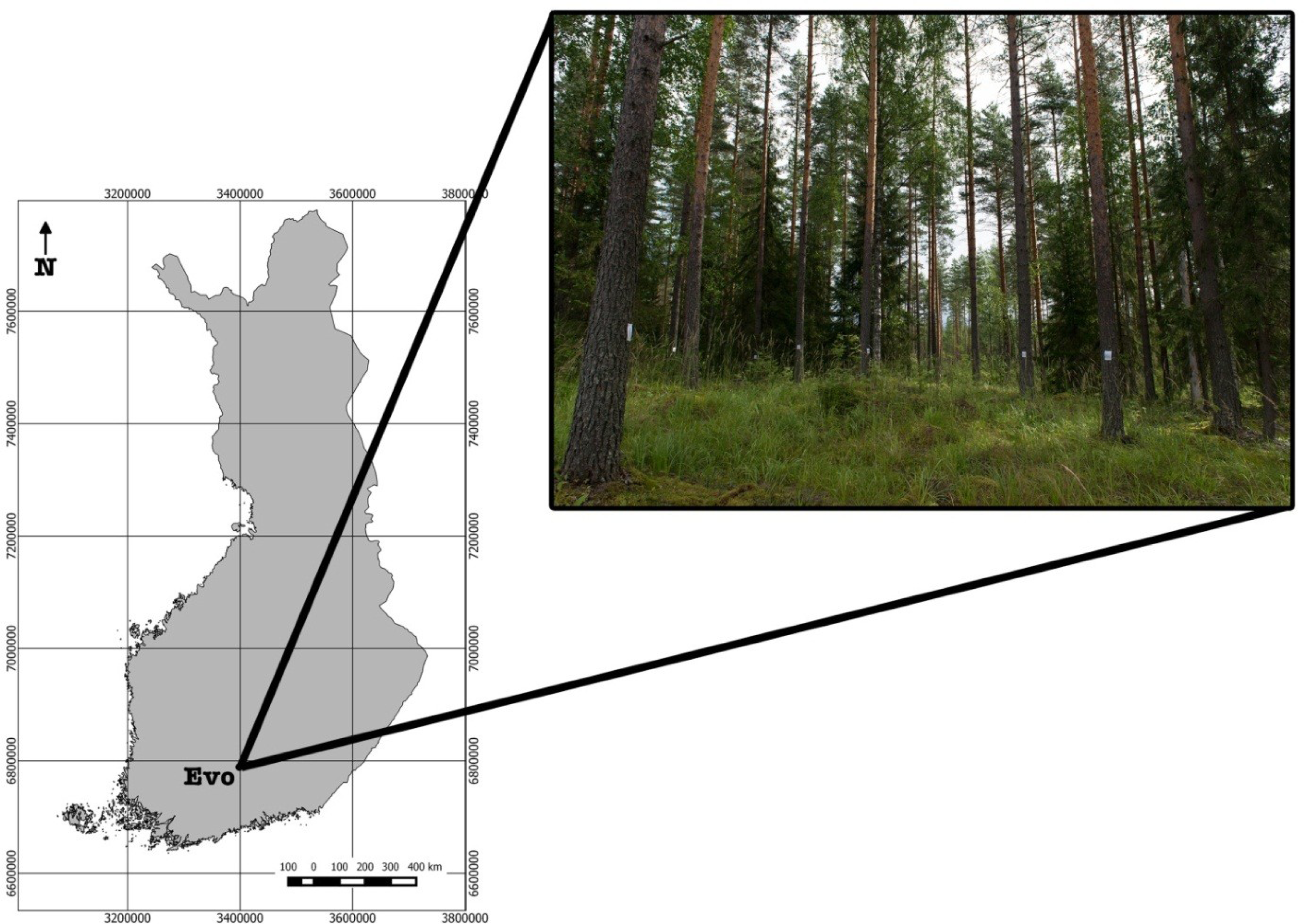
2.1. Study Area and Field Measurements

The study area (Figure 1) is located in Evo, southern Finland (61.19°N, 25.11°E). The area belongs to the southern Boreal zone and comprises approximately 2000 ha of mainly managed forest. The study site was a forest stand, which was approximately 2 hectares in size, and the main tree species was Scots pine (Pinus sylvestris L.). The site type of the stand was Myrtillus-type (medium-rich mineral soil forest). The mean age of the pine trees was approximately 75 years, and the forest management history included thinnings and two fertilizations. Field measurements were conducted for 144 sample trees from the stand in the fall of 2012. Trees were marked and numbered in the field, and diameter was measured with steel calipers from two directions perpendicular to each other at the height of 1.3 m. Tree height was measured with a Haglöf Vertex laser rangefinder (Haglöf Sweden AB, Långsele, Sweden). The mean height and diameter of the sample trees were 24.7 m and 29.8 cm, respectively. More detailed statistics of the sample trees are presented in

Table 1. Tree statistics calculated from the field measurements.

	Min	Mean	Max	SD
Diameter, cm	18.3	29.8	41.0	4.4
Height, m	19.0	24.7	28.6	1.6

.

2.2. Terrestrial Laser Scanning

The TLS data were collected in the fall of 2012 with a Leica HDS6100 TLS system (Leica Geosystem AG, Heerbrugg, Switzerland). The HDS6100 is a 690-nm phase-based continuous-wave laser scanner with a 360° × 310° field of view upwards, and its data-acquisition rate is 508,000 points per second. The distance measurement accuracy is ±2 mm at a distance of 25 m. The circular-beam diameter at the exit and the beam divergence are 3 mm and 0.22 mrad, respectively. The point spacing is 6.3 mm at 10 m (with an angular resolution of 0.009°). In all, 45 scans were made and coregistered to cover the whole stand and sample trees. The reference targets (spheres) were used to ensure accurate coregistration, which was done using Leica’s Cyclone software (Leica Geosystems AG. Heerbrugg). TLS data were also registered to the external coordinate system (ETRS-35TMFIN), using reference target locations and scanning locations measured with the GNSS.

2.3. Airborne Laser Scanning

The ALS datasets were acquired in midsummer, 2011 and 2012. The ALS campaign in 2011 was acquired with a Leica ALS50-II scanner. The flying altitude was 1000 m above ground level, and the pulse density was approximately 9 pulses per square meter. The National Land Survey of Finland (NLS) conducted the ALS campaign in the study area with a Leica ALS50 scanner in 2012. The flying altitude was 2200 m, and the pulse density was around 0.8 pulses per square meter. In both of the data sets, a digital terrain model (DTM) and, consequently, heights above ground level were computed by the data provider.

2.4. Aerial Images and Digital Surface Model Generation

The aerial imagery was acquired in August 2009. The imaging sensor used was a Microsoft UltracamXp with a stereoscopic forward overlap of 70% and side overlap of 30%. The area was covered by 51 images in total. Images were taken from three separate flight lines covering 17 images each. The ground-sample distance (GSD) was approximately 0.25 m. The images were delivered as 16-bit RGB (red, green, blue) and color infrared (CIR) composites. The image orientation was completed by the data vendor (FM International Oy, Helsinki, Finland). Based on the image-orientation report provided, the RMSE accuracy of the orientation (validated with seven ground control points) was 4.3 cm, 3.1 cm and 9.1 cm in the X, Y and Z directions, respectively. For the development of a high-spatial resolution (0.5 m) DSI-based digital surface model (DSM), the Next-Generation Automatic Terrain Extraction (NGATE) module of the software, SOCET SET (from BAE Systems), was used. The ALS-based DTM was subtracted from the DSI-based DSM to create CHM. Further details are given in [32,33].

2.5. Harvester Measurements

Harvester measurements were collected in the fall of 2012. Each sample tree was cut down and cut into saw logs and pulpwood. Trees were also linked to field reference trees during this process. The following parameters were measured with a harvester information system: saw log and pulpwood volume and length and bucking information. The upper diameter limit for logs was 16 cm and for pulpwood, 7 cm.

Table 2. Description of the sample trees measured and cut with a harvester.

	Min	Mean	Max	SD
Saw log volume (dm3)	0.0	695.1	1531.9	268.4
Pulpwood volume (dm3)	0.0	117.7	914.8	113.3

summarizes the harvester measurements.

2.6. Multisource Single-Tree Inventory

We tested MS-STI by using three different kinds of remote-sensing materials in the prediction of the stem attributes and diameter distribution. MS-STI-1 uses ALS data with ∼9 pulses per m² in the extraction of the predictor variables, whereas MS-STI-2 uses ALS data with a pulse density of ∼1 pulses per m² (Section 2.3). MS-STI-3 uses CHM derived from digital stereo imagery in the extraction of the predictors (Section 2.4). All of the three MS-STIs use the same stem map derived from the TLS and GNSS measurements as the input information (Section 2.6.1). MS-STI is described in more detail in the following sections.

2.6.1. Tree Map-Assisted Extraction of Predictor Variables

The location of each tree was determined manually from the TLS point cloud and then used as auxiliary information when extracting predictors for single trees. TLS point clouds were processed in scan groups, and trees were searched within each group using visual interpretation. The process was performed through the following steps: (1) the point cloud of each scan group was imported into TerraScan by thinning the point cloud by 50%; (2) points from an approximately 1.3-m height (between 1.25 m and 1.35 m to be exact) were classified into a horizontal “slice” for identifying tree trunks; (3) tree trunks were detected and marked within the slice; and (4) location and DBH information were recorded for all the trees. In MS-STI-1, dense, 9 pulses per m² ALS data was used, and thus, CHM was first segmented using watershed segmentation [9,34,35]. Segments were then linked to the trees. If there was more than one tree within a segment, the segment was split equally to represent both of the trees. In MS-STI-2 and MS-STI-3, predictors were extracted using circular polygons around the tree location. The area of the polygons was fixed to 7 m² to cover height observations close to the tree stem and to avoid overlapping with other trees. The size of the polygon was not further tested.

Statistical metrics describing tree crown density and tree height were calculated from the ALS or DSI data (

Table 3. Statistics, such as minimum (min), maximum (max), range, mean and standard deviation (SD) calculated from the extracted predictor variables. The suffix “_fi” means that only the first returns were used for calculations. vege, vegetation ratio; Hmax, height maximum; Hmean, average height; Hstd, height standard deviation; h10–h90, point height at the 10th–90th percentile (h10–h90); p10–p90, crown-cover metrics as a proportion of point heights below a certain relative tree height. MS-STI, multisource single-tree inventory.

	MS-STI-1					MS-STI-2					MS-STI-3
Variable	Min	Max	Range	Mean	SD	Min	Max	Range	Mean	SD	Min	Max	Range	Mean	SD
Hmax	18.1	28.4	10.3	23.6	1.5	16.9	28.5	11.6	23	1.7	9.6	28.6	19	22.2	2.6
Hmean	11.5	20.5	9	16.7	2	12.9	25.9	13	20	2.3	2.6	25.2	22.5	19.3	3.6
Hstd	1.6	9.5	7.8	5.7	1.6	0.4	9.9	9.5	3.4	2.5	0.4	6.1	5.7	1.7	1.2
vege	0.2	0.9	0.7	0.7	0.1	0.5	1	0.5	1	0.1	0.6	1	0.4	1	0.1
CV	0.1	0.8	0.7	0.4	0.1	0	0.7	0.7	0.2	0.2	0	1.2	1.2	0.1	0.2
h10	0.8	18.9	18.1	8.1	5.5	1.3	24	22.7	16.1	5.6	0.7	23.3	22.6	17.1	4.7
h20	1.9	20.2	18.3	12.7	4.9	2.1	25	22.9	18.1	4.3	0.9	23.9	22.9	17.9	4.4
h30	2.2	20.7	18.5	15.5	3.8	3.5	25.3	21.8	19.6	3	1	24.3	23.3	18.5	4
h40	3.8	21.5	17.7	17.2	2.7	12.4	25.5	13	20.5	2	1.2	24.7	23.5	19	3.8
h50	4.1	22.3	18.2	18.3	2.3	13.8	25.7	11.9	21.1	1.8	1.4	24.8	23.4	19.5	3.7
h60	13.8	22.9	9.1	19.4	1.7	15.7	26.3	10.6	21.5	1.6	1.6	25.1	23.5	19.9	3.5
h70	15.4	23.9	8.5	20.3	1.5	16.7	26.9	10.2	21.8	1.6	1.7	25.5	23.8	20.2	3.3
h80	15.4	25.2	9.7	21.1	1.5	16.9	27.3	10.4	22.2	1.6	3.7	26.4	22.8	20.7	3
h90	17	26.5	9.5	22.1	1.5	16.9	27.9	11	22.6	1.6	6.7	27.8	21.1	21.2	2.8
p10	0	0.3	0.3	0.1	0.1	0	0.3	0.3	0	0.1	0	0.8	0.8	0	0.1
p20	0	0.5	0.5	0.1	0.1	0	0.4	0.4	0	0.1	0	0.8	0.8	0	0.1
p30	0	0.5	0.5	0.1	0.1	0	0.4	0.4	0	0.1	0	0.8	0.8	0	0.1
p40	0	0.5	0.5	0.1	0.1	0	0.4	0.4	0.1	0.1	0	0.9	0.9	0	0.1
p50	0	0.6	0.6	0.2	0.1	0	0.4	0.4	0.1	0.1	0	0.9	0.9	0	0.2
p60	0	0.6	0.6	0.2	0.1	0	0.4	0.4	0.1	0.1	0	0.9	0.9	0.1	0.2
p70	0	0.7	0.7	0.3	0.1	0	0.5	0.5	0.1	0.1	0	0.9	0.9	0.1	0.2
p80	0.1	0.8	0.7	0.5	0.1	0	0.7	0.7	0.2	0.2	0	1	1	0.1	0.2
p90	0.4	0.9	0.6	0.8	0.1	0	0.8	0.8	0.4	0.2	0	1	1	0.1	0.2
Hmax_fi	18.1	28.4	10.3	23.6	1.5	16.9	28.5	11.6	23	1.7
Hmean_fi	12.7	22.1	9.5	18.1	1.8	16.9	26.4	9.6	21.1	1.6
Hstd_fi	1.2	9.5	8.3	4.5	1.6	0.4	9.3	8.9	1.9	1.4
vege_fi	0.3	1	0.7	0.8	0.1	0.5	1	0.5	1	0.1
CV_fi	0.1	0.7	0.7	0.3	0.1	0	0.6	0.5	0.1	0.1
h10_fi	1.1	20.2	19.2	12.3	5.1	3.8	25.1	21.3	19.1	2.6
h20_fi	2.1	20.8	18.7	15.7	3.5	8.4	25.4	17	20.1	2
h30_fi	3.1	21.5	18.4	17.1	2.9	16.4	25.5	9.1	20.6	1.7
h40_fi	4	22.2	18.2	18.2	2.1	16.9	25.7	8.8	21.1	1.6
h50_fi	13.4	22.6	9.2	19.1	1.6	16.9	26.2	9.3	21.4	1.6
h60_fi	15.2	23.7	8.4	19.9	1.5	16.9	26.7	9.8	21.7	1.6
h70_fi	15.4	24.1	8.8	20.7	1.5	16.9	27.1	10.2	22	1.6
h80_fi	15.4	25.4	9.9	21.4	1.5	16.9	27.5	10.6	22.3	1.5
h90_fi	17	26.8	9.8	22.2	1.5	16.9	28	11.1	22.7	1.6
p10_fi	0	0.2	0.2	0	0	0	0.1	0.1	0	0
p20_fi	0	0.5	0.5	0.1	0.1	0	0.1	0.1	0	0
p30_fi	0	0.5	0.5	0.1	0.1	0	0.3	0.3	0	0
p40_fi	0	0.5	0.5	0.1	0.1	0	0.3	0.3	0	0
p50_fi	0	0.5	0.5	0.1	0.1	0	0.3	0.3	0	0
p60_fi	0	0.5	0.5	0.1	0.1	0	0.3	0.3	0	0
p70_fi	0	0.6	0.6	0.2	0.1	0	0.3	0.3	0	0.1
p80_fi	0	0.8	0.7	0.5	0.1	0	0.5	0.5	0.1	0.1
p90_fi	0.3	0.9	0.6	0.8	0.1	0	0.8	0.8	0.3	0.2

). The DSI-derived CHM raster layer was treated as an XYZ point cloud, respectively, to the ALS point cloud. First, point heights over 0.5 m were classified as coming from the vegetation (i.e., tree), and a vegetation ratio (vege) was then calculated as a ratio between vegetation point heights and all point heights within a crown segment. The other extracted metrics were: the maximum (Hmax), average (Hmean), standard deviation (Hstd) and coefficient of variation of point heights (CV); point height at the 10th–90th percentile (h10–h90) and crown-cover metrics as a proportion of point heights below a certain relative tree height (p10–p90). Only the points belonging to vegetation (that is, a height over 0.5 m) were used in calculating these metrics. The metrics were extracted from the ALS data using first returns and all returns separately.

2.6.2. Estimation of Tree quality Variables

Height, diameter, saw log volume and pulpwood volume were predicted by means of ALS and DSI metrics using the nearest-neighbor (NN) approach. Tree variables measured in the field (height, diameter) or recorded with a harvester (saw log volume, pulpwood volume) were used as target observations, and tree-specific metrics derived from ALS and DSI data were used as predictors. The random forest approach (RF, [36]) was applied in the NN search. Based upon the quality of results and the desirable statistical characteristics (i.e., the capability to predict multiple-response variables simultaneously, to use a large number of predictors without the problem of over fitting and to evaluate the accuracy with built-in functionality), the use of RF in NN estimation of forest variables is increasingly common (e.g., [9,37]). Hudak et al. [37] demonstrated that the RF method is more robust and flexible for forest-variable prediction when compared to other NN distance measures, such as Euclidian distance, Mahalanobis distance or canonical-correlation analysis. In the RF method, several regression trees are generated by drawing a replacement from two-thirds of the data for training and one-third for testing for each tree. The samples that are not included in training are called out-of-bag samples, and they can act as a testing set in the approach. The measure of nearness in RF is defined based on the observational probability of ending up in the same terminal node in classification. The R statistical computing environment [38] and yaImpute library [39] were applied in the RF predictions. The yaImpute library is tailored to NN forest attribute estimation.

In the present study, 1200 regression trees were generated, and the square root of the number of predictor variables was picked randomly at the nodes of each regression tree. Three-hundred regression trees per predicted variable were suggested by Hudak et al. [37]. Randomness was taken into account by running the RF method 100 times. The final result was the average of these runs. The number of neighbors was set to one to keep the original variance in the data (see, e.g., [37]).

Prior to the final modeling, RF was used to reduce the number of predictor variables. The aim of the variable reduction was to build up parsimonious models that are capable of accurate predictions. A step-wise looping procedure was used to iterate RF, discarding the least important of the candidate variables at each iteration, based on the variable importance, until only a single predictor variable remained. RMSEs were calculated for each predictor variable combination and analyzed.

2.7. Accuracy Assessment at the Single-Tree and Sub-Stand Level

In this study, predictors and target observations were available for all of the trees. Therefore, the accuracy of the predicted variables at the tree level was evaluated by calculating bias and RMSE using out-of-the-bag samples. The relative bias and RMSE were calculated according to the sampled mean of the variable in question. At the stand level, stem-diameter distribution, tree-height distribution, saw-log recovery and pulpwood recovery were compiled from the tree-level predictions and compared to the field and harvester measures. Differences are reported for saw wood and pulpwood recoveries. The goodness of fit of the predicted stem-diameter and height distributions was evaluated by using an error index proposed by Packalén and Maltamo [40]:

$$e=\sum _{i=1}^{k}0.5\left|\frac{f_i}{N}-\frac{{\widehat{f}}_i}{\widehat{N}}\right|$$

(1)

where f_i is the true and f̂_i is the predicted stem number in class i, k is the number of classes or bins and N is the true and N̂ the predicted stem number of all diameter classes. A bin size of 2 cm was used for diameter and 1 m for height. The error index is modified from the one suggested by Reynolds et al. [41]. Frequency differences are multiplied by 0.5 in Equation (1) to scale the error index to between 0 and 1, 0 meaning a perfect fit and 1 meaning that the distributions do not overlap at all.

3. Results

In total, MS-STI-1 and MS-STI-2 had 46 possible predictor variables and MS-STI-3 had 23. After the reduction of the predictor variables, MS-STI-1 had 16, MS-STI-2 had 15 and MS-STI-3 had 10 predictor variables (

Table 4. Selected predictor variables.

Variable	MS-STI-1	MS-STI-2	MS-STI3
Hmax	x	x	x
Hmean			x
CV		x	x
h20	x		x
h30		x
h40		x	x
h50		x	x
h60	x	x	x
h70		x	x
h80	x	x	x
h90	x	x	x
p10	x
p20	x
p30	x
p80	x
Hmean_fi		x
vege_fi	x
h30_fi	x
h40_fi	x
h50_fi		x
h60_fi		x
h70_fi	x	x
h80_fi	x	x
h90_fi	x	x
p80_fi	x

). In general, the prediction accuracy was not overly sensitive to the number of the used predictor variables. For example, the RMSEs varied in MS-STI-1 from 10.7% to 15.6% in stem diameter and from 5.0% to 6.1% in tree height when the number of predictors varied from 46 to two.

3.1. Prediction Accuracy of Tree Height, Diameter, Stem Volume and Timber Assortments

Tree height, stem diameter, saw log volume and pulpwood volume were all predicted simultaneously using RF. All of the three MS-STIs provided meter-class accuracy for tree height with low biases (

Table 5. Accuracy of the MS-STI in the prediction of tree quality variables.

	k	Bias	Bias-%	RMSE	RMSE-%
Tree height (m)
MS-STI-1	1	−0.1	−0.2	1.2	4.7
MS-STI-2	1	0.0	0.0	1.0	4.2
MS-STI-3	1	0.0	−0.1	1.3	5.3
Tree diameter (cm)
MS-STI-1	1	0.1	0.3	3.2	10.9
MS-STI-2	1	−0.1	−0.4	5.9	19.9
MS-STI-3	1	0.2	0.6	4.7	16.1
Saw log volume (dm3)
MS-STI-1	1	1.5	0.2	200.3	28.7
MS-STI-2	1	−2.8	−0.4	304.8	43.5
MS-STI-3	1	9.0	1.3	284.3	40.7
Pulpwood volume (dm3)
MS-STI-1	1	3.2	2.7	159.4	134.3
MS-STI-2	1	12.6	10.6	148.6	125.1
MS-STI-3	1	−3.5	−3.0	159.8	135.3

). The variation in tree height prediction accuracy between the MS-STIs was marginal, and the RMSEs varied only from 4.2% to 5.3%. In stem diameter and saw log volume predictions, MS-STI-1 provided the most accurate estimates with RMSEs of 3.2 cm (10.9%) and 200.3 dm³ (28.7%), respectively. Pulpwood volume prediction was the most unreliable, with all of the MS-STIs and the RMSE varying from 125.1% to 135.3% and the biases from −3.0% to 10.6%.

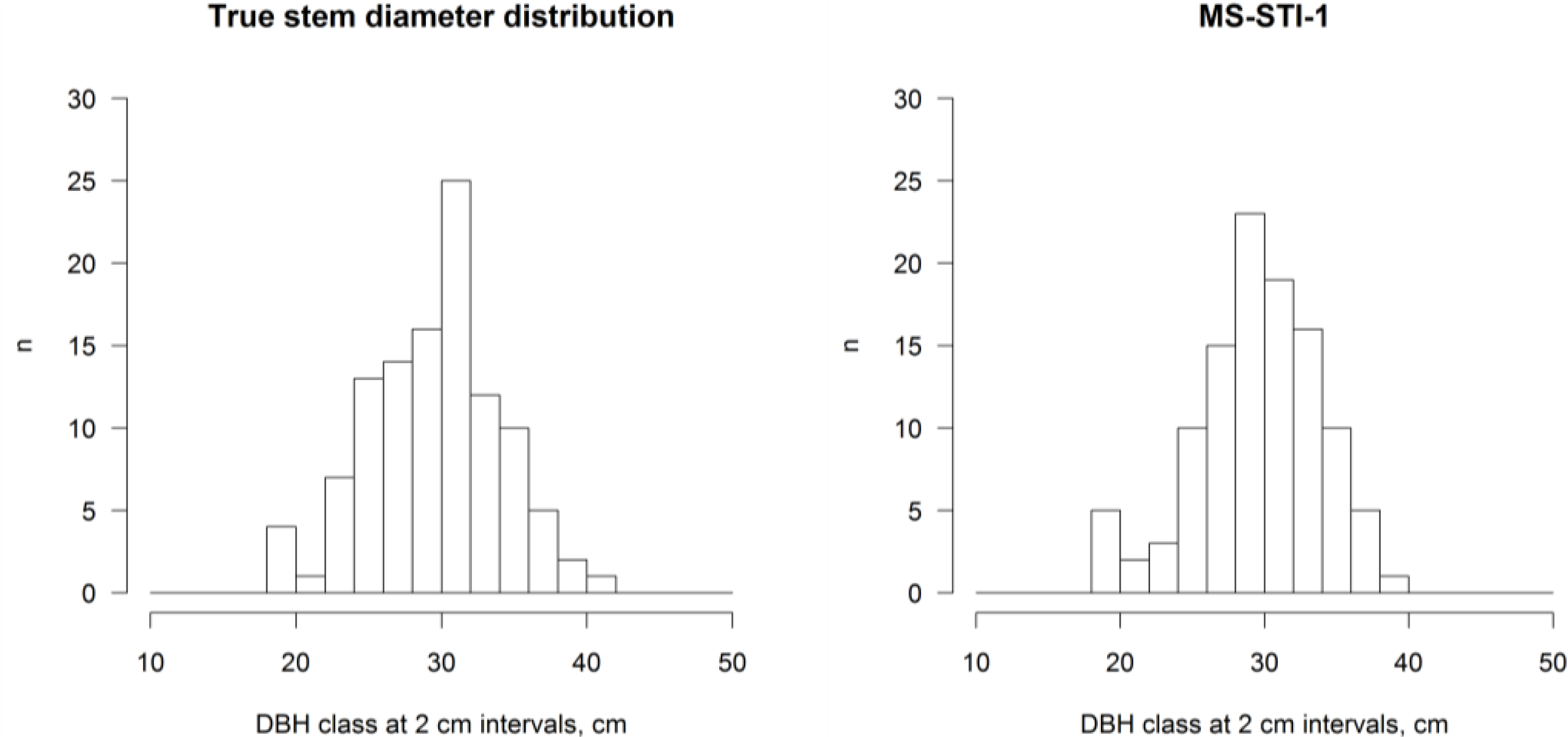
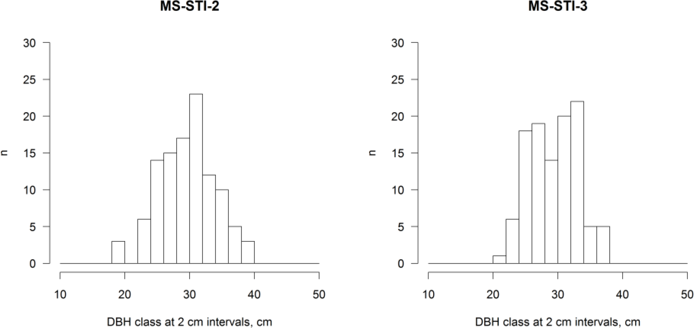
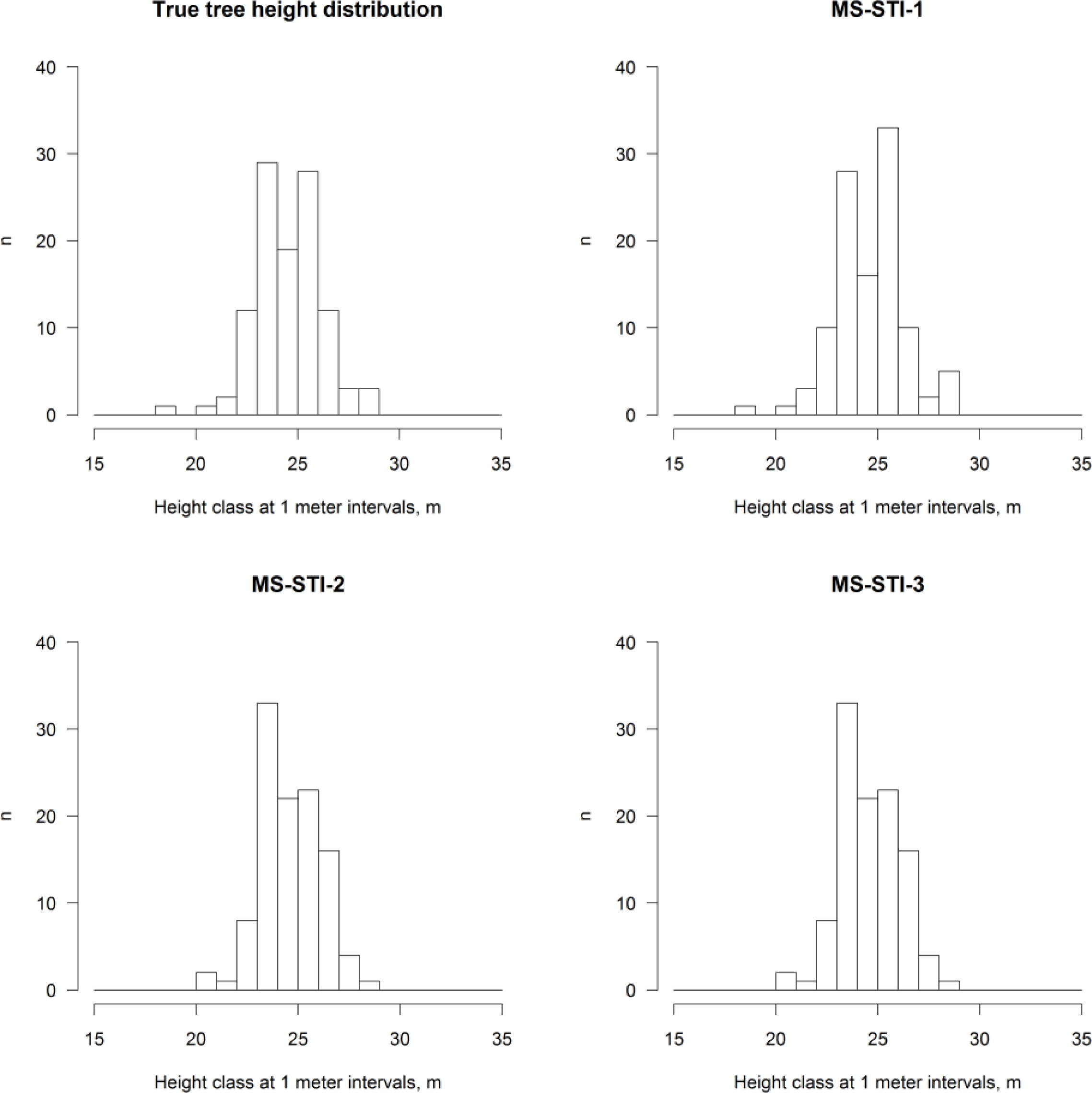
3.2. Comparisons of Stem-Distribution Series and Accuracy in Prediction of Timber Assortments at the Sub-Stand Level

All of the MS-STIs provided accurate estimates for saw log and pulpwood recoveries at the stand level. MS-STI-1’s saw log recovery estimate differed by only 0.2% from the true harvester-measured recovery. The respective difference in pulpwood recovery was 2.7%. Saw log recoveries with MS-STI-2 and MS-STI-3 differentiated −0.4% and 1.3%, as the respective differences in pulpwood recoveries were 10.6% and −3.0%. MS-STI-1 and MS-STI-2 provided the most accurate stem-diameter distribution (Figure 2), while the MS-STI-1 was clearly most accurate in predicting tree-height distribution (Figure 3). Error indices for the predicted diameter distributions were 0.10, 0.11 and 0.15 for MS-STI-1, MS-STI-2 and MS-STI-3, respectively. The error indices for the predicted height distributions were 0.06, 0.10 and 0.15 for MS-STI-1, MS-STI-2 and MS-STI-3.

4. Discussion

This study was a pre-investigation in developing the next generation’s detailed forest-inventory process for countries applying intensive small-scale forestry. Here, we developed and demonstrated a use of MS-STI in which two major bottlenecks, tree detection and tree species recognition, in the current ALS-based STI are avoided. In addition to the ALS data, MS-STI requires an existing tree map with tree species information as the input information. With this information as input, it is possible to avoid the challenging steps of tree detection and tree species recognition.

In STI studies (e.g., [5,21,22]), the results have been promising, due to suitable forest conditions (mature stand) and/or validation data having been selected based on correct matching between ALS and field data. STI results have varied considerably depending on the forest conditions [9,10,12,16]. A practical solution for reliable STI has not been suggested so far. We believe that the existing tree map could be the solution. It should be noted that our study was also carried out in forest conditions that favored STI. The data were collected from a single mature Scot’s pine stand. Thus, we were not studying tree species classification from TLS data or the prediction of species-specific tree quality variables. However, with the existing tree map, it can be assumed that MS-STI is capable of providing robust estimates in various forest conditions, and we will investigate that in forthcoming studies. A tree map with species information is a challenging prerequisite, but the recent developments in mobile 2D and 3D laser scanning indicates that the solution is within reach [23–30]. In our study, the tested input tree map was produced by TLS and using GNSS with an expected accuracy of below 0.1 m. In operational forest management, tree mapping would be carried out after or during the thinning, which is the earliest stage to apply MS-STI. After that, tree-level information could be used for optimizing wood supply, spatial modeling of the growth and even in the guidance of bucking.

Predictors for tree quality attributes were extracted from ALS data or DSI for mapped tree locations. Stem distribution was compiled by summing single-tree measures. The accuracy of the MS-STI was validated using harvester data (timber assortments) and field measures (diameter, height). MS-STI provided accurate estimates for diameter, height and timber assortments. It should be noted that comparing the results of this kind of study to other studies is only suggestive and highly data dependent. However, after this reminder, we can point out that our results are promising and on the same level or even better than the results obtained earlier using STI methods [5,9,20–22]. For example, the obtained accuracies for tree quality variables were similar to the accuracies obtained by Maltamo et al. [21] or Lindberg et al. [20]. We could have obtained even lower RMSEs by enlarging the number of neighbors used in the estimation, but that would have contracted the estimated stem distribution. Accurate stem distribution is desired for logging optimization, and the forestry industry is highly interested in obtaining these prior loggings [4,22,40]. With a k-value of one, we were able to retain the original variance in tree quality variables as well as possible in the RF estimation. At the stand level, we obtained more accurate estimates for saw log and pulpwood recoveries by using MS-STI than had been obtained by Peuhkurinen et al. [22] or Holmgren et al. [5]. Peuhkurinen et al. [22] estimated saw wood recovery to be under 0.5% and pulpwood with a 22% difference to the harvester measurements. MS-STI-1’s saw log recovery estimate differed with only 0.2% from the true harvester-measured recovery, and the difference in pulpwood recovery was 2.7%. Estimates for timber assortment were also much more accurate than what had previously been obtained by using an area-based approach [4]. In general, the obtained stem-diameter distributions were more accurate than in Packalén and Maltamo [40] and Vauhkonen et al. [6] in which a comparable error index was used. Packalén and Maltamo [40] used ABA to predict species-specific stem-diameter distributions, and error indices varied from 0.21 to 0.34. Vauhkonen et al. [6] used the STI technique and tree-list imputation method; error indices varied from 0.33 to 0.40 for all of the trees, and the species-specific error indices varied from 0.9 to 0.23. The error indices we obtained with MS-STI varied from 0.10 to 0.15.

One of the most intriguing considerations with MS-STI is that it is capable of producing accurate estimates even with DSI-derived CHM data or low-pulse density ALS data (0.5 pulses per m² used here in MS-STI-2). This is promising for forest resource information updates. Once the tree map is produced by using 2D or 3D laser techniques, there are many possible options for updating forest data. For example, an existing tree map (acquired during the thinning) could be used prior to the final cutting when tree quality attributes and logging recoveries are predicted using the newest possible 3D remote-sensing data. Then, the detailed tree information could be used for optimizing wood supply and even in the guidance of bucking.

In forthcoming studies, MLS- and TLS-based tree mapping and tree species detection should be developed further in conjunction with MS-STI. The required accuracy of the tree map also requires further study, especially if MS-STI is carried out using DSI or low-pulse density ALS data.

5. Conclusion

Here, we developed and demonstrated a use of multisource single-tree inventory (MS-STI) in which two major bottlenecks, tree detection and tree species recognition, in the current airborne laser scanning (ALS)-based single-tree inventory, are avoided. In addition to the ALS or other detailed airborne 3D data (such as the digital stereo imagery-derived point cloud), MS-STI requires an existing tree map with tree species information as the input information. With this information as the input, it is possible to avoid the challenging steps of tree detection and tree species recognition. The tree map is then used to support the extraction of the predictors and the estimation of the tree quality attributes from airborne 3D data. With this approach, the root mean square errors (RMSEs) for tree height, diameter, saw log volume and pulpwood volume varied from 4.2% to 5.3%, from 10.9% to 19.9%, from 28.7% to 43.5% and from 125.1% to 134.3%, respectively, depending on the used airborne 3D data. Stand-level saw log recoveries differed from −2.2% to 1.3% from the harvester measurements, as the respective differences in pulpwood recovery were between −3.0% and 10.6%. The obtained results are promising and on the same level or even better than the results obtained in previous studies. We conclude that MS-STI is capable of providing realistic stem distributions and accurate estimates for tree quality variables with ALS data or digital stereo imagery if an accurate tree map is available.

References

1. Næsset, E. Practical large-scale forest stand inventory using a small-footprint airborne scanning laser. Scand. J. Forest Res 2004, 19, 164–179. [Google Scholar]
2. White, J.; Wulder, M.; Vastaranta, M.; Coops, N.; Pitt, D.; Woods, M. The utility of image-based point clouds for forest inventory: A comparison with airborne laser scanning. Forests 2013, 4, 518–536. [Google Scholar]
3. Vastaranta, M. Forest Mapping and Monitoring Using Active 3D Remote Sensing. Ph.D. Dissertation. University of Helsinki, Helsinki, Finland. 2012. [Google Scholar]
4. Holopainen, M.; Vastaranta, M.; Rasinmäki, J.; Kalliovirta, J.; Mäkinen, A.; Haapanen, R.; Melkas, T.; Yu, X.; Hyyppä, J. Uncertainty in timber assortment estimates predicted from forest inventory data. Eur. J. Forest Res 2010, 129, 1131–1142. [Google Scholar]
5. Holmgren, J.; Barth, A.; Larsson, H.; Olsson, H. Prediction of stem attributes by combining airborne laser scanning and measurements from harvesters. Silva Fennica 2012, 46, 227–239. [Google Scholar]
6. Vauhkonen, J.; Packalen, P.; Malinen, J.; Pitkänen, J.; Maltamo, M. Airborne laser scanning based decision support for wood procurement planning. Scand. J. Forest Res 2013. [Google Scholar] [CrossRef]
7. Hyyppä, J.; Inkinen, M. Detecting and estimating attributes for single trees using laser scanner. Photogramm. J. Finl 1999, 16, 27–42. [Google Scholar]
8. Hyyppä, J.; Yu, X.; Hyyppä, H.; Vastaranta, M.; Holopainen, M.; Kukko, A.; Kaartinen, H.; Jaakkola, A.; Vaaja, M.; Koskinen, J. Advances in forest inventory using airborne laser scanning. Remote Sens 2012, 4, 1190–1207. [Google Scholar]
9. Yu, X.W.; Hyyppa, J.; Vastaranta, M.; Holopainen, M.; Viitala, R. Predicting individual tree attributes from airborne laser point clouds based on the random forests technique. ISPRS J. Photogramm. Remote Sens 2011, 66, 28–37. [Google Scholar]
10. Kaartinen, H.; Hyyppä, J.; Yu, X.; Vastaranta, M.; Hyyppä, H.; Kukko, A.; Holopainen, M.; Heipke, C.; Hirschmugl, M.; Morsdorf, F. An international comparison of individual tree detection and extraction using airborne laser scanning. Remote Sens 2012, 4, 950–974. [Google Scholar]
11. Vastaranta, M.; Holopainen, M.; Yu, X.; Hyyppä, J.; Mäkinen, A.; Rasinmäki, J.; Melkas, T.; Kaartinen, H.; Hyyppä, H. Effects of individual tree detection error sources on forest management planning calculations. Remote Sens 2011, 3, 1614–1626. [Google Scholar]
12. Vauhkonen, J.; Ene, L.; Gupta, S.; Heinzel, J.; Holmgren, J.; Pitkänen, J.; Solberg, S.; Wang, Y.; Weinacker, H.; Hauglin, K.M. Comparative testing of single-tree detection algorithms under different types of forest. Forestry 2012, 85, 27–40. [Google Scholar]
13. Falkowski, M.J.; Smith, A.M.; Gessler, P.E.; Hudak, A.T.; Vierling, L.A.; Evans, J.S. The influence of conifer forest canopy cover on the accuracy of two individual tree measurement algorithms using lidar data. Can. J. Remote Sens 2008, 34, S338–S350. [Google Scholar]
14. Persson, A.; Holmgren, J.; Söderman, U. Detecting and measuring individual trees using an airborne laser scanner. Photogramm. Eng. Remote Sens 2002, 68, 925–932. [Google Scholar]
15. Pirotti, F. Assessing a template matching approach for tree height and position extraction from lidar-derived canopy height models of pinus pinaster stands. Forests 2010, 1, 194–208. [Google Scholar]
16. Pitkänen, J.; Maltamo, M.; Hyyppä, J.; Yu, X. Adaptive methods for individual tree detection on airborne laser based canopy height model. Int. Arch. Photogramm. Remote Sens. Spat. Inf. Sci 2004, 36, 187–191. [Google Scholar]
17. Gupta, S.; Koch, B.; Weinacker, H. Tree species detection using full waveform lidar data in a complex forest. Int. Arch. Photogramm. Remote Sens. Spat. Inf. Sci 2010, 38, 249–254. [Google Scholar]
18. Wang, Y.; Weinacker, H.; Koch, B.; Sterenczak, K. Lidar point cloud based fully automatic 3D single tree modelling in forest and evaluations of the procedure. Int. Arch. Photogramm. Remote Sens. Spat. Inf. Sci 2008, 37, 45–51. [Google Scholar]
19. Kaartinen, H.; Hyyppä, J. EuroSDR/ISPRS Project, Commission II “Tree Extraction”. Final Report; EuroSDR (European Spatial Data Research): Frankfurt a.M., Germany, 2008. [Google Scholar]
20. Lindberg, E.; Holmgren, J.; Olofsson, K.; Olsson, H. Estimation of stem attributes using a combination of terrestrial and airborne laser scanning. Eur. J. Forest Res 2012, 131, 1917–1931. [Google Scholar]
21. Maltamo, M.; Peuhkurinen, J.; Malinen, J.; Vauhkonen, J.; Packalén, P.; Tokola, T. Predicting tree attributes and quality characteristics of Scots pine using airborne laser scanning data. Silva Fennica 2009, 43, 507–521. [Google Scholar]
22. Peuhkurinen, J.; Maltamo, M.; Malinen, J.; Pitkanen, J.; Packalen, P. Preharvest measurement of marked stands using airborne laser scanning. Forest Sci 2007, 53, 653–661. [Google Scholar]
23. Forsman, P.; Halme, A. 3-D mapping of natural environments with trees by means of mobile perception. IEEE Trans. Robot 2005, 21, 482–490. [Google Scholar]
24. Hellström, T.; Lärkeryd, P.; Nordfjell, T.; Ringdahl, O. Autonomous forest vehicles: Historic, envisioned, and state-of-the-art. Int. J. Forest Eng 2009, 20, 31–38. [Google Scholar]
25. Jutila, J.; Kannas, K.; Visala, A. Tree Measurement in Forest by 2D Laser Scanning. In Proceedings of 2007 International Symposium on Computational Intelligence in Robotics and Automation, CIRA 2007, Jacksonville, FL, USA, 20–23 June 2007; pp. 491–496.
26. Liang, X.; Litkey, P.; Hyyppä, J.; Kaartinen, H.; Vastaranta, M.; Holopainen, M. Automatic stem mapping using single-scan terrestrial laser scanning. IEEE Trans. Geosci. Remote Sens 2012, 50, 661–670. [Google Scholar]
27. Miettinen, M.; Ohman, M.; Visala, A.; Forsman, P. Simultaneous Localization and Mapping for Forest Harvesters. In Proceedings of 2007 IEEE International Conference on Robotics and Automation, Roma, Italy, 10–14 April 2007; pp. 517–522.
28. Ringdahl, O.; Hohnloser, P.; Hellström, T.; Holmgren, J.; Lindroos, O. Enhanced algorithms for estimating tree trunk diameter using 2D laser scanner. Remote Sens 2013, 5, 4839–4856. [Google Scholar]
29. Öhman, M.; Miettinen, M.; Kannas, K.; Jutila, J.; Visala, A.; Forsman, P. Tree Measurement and Simultaneous Localization and Mapping System for Forest Harvesters. In Field and Service Robotics; Springer: Heidelberg, Germany, 2008; pp. 369–378. [Google Scholar]
30. Holopainen, M.; Kankare, V.; Vastaranta, M.; Liang, X.; Lin, Y.; Vaaja, M.; Yu, X.; Hyyppä, J.; Hyyppä, H.; Kaartinen, H. Tree mapping using airborne, terrestrial and mobile laser scanning—A case study in a heterogeneous urban forest. Urban Forestry Urban Green 2013, 12, 546–553. [Google Scholar]
31. Hyyppa, J.; Jaakkola, A.; Hyyppa, H.; Kaartinen, H.; Kukko, A.; Holopainen, M.; Zhu, L.; Vastaranta, M.; Kaasalainen, S.; Krooks, A. Map Updating and Change Detection Using Vehicle-Based Laser Scanning. In Proceedings of IEEE 2009 Joint Urban Remote Sensing Event, Shanghai, China, 20–22 May 2009; pp. 1–6.
32. Järnstedt, J.; Pekkarinen, A.; Tuominen, S.; Ginzler, C.; Holopainen, M.; Viitala, R. Forest variable estimation using a high-resolution digital surface model. ISPRS J. Photogramm. Remote Sens 2012, 74, 78–84. [Google Scholar]
33. Vastaranta, M.; Wulder, M.A.; White, J.C.; Pekkarinen, A.; Tuominen, S.; Ginzler, C.; Kankare, V.; Holopainen, M.; Hyyppä, J.; Hyyppä, H. Airborne laser scanning and digital stereo imagery measures of forest structure: Comparative results and implications to forest mapping and inventory update. Can. J. Remote Sens 2013, 39, 1–14. [Google Scholar]
34. Kankare, V.; Vastaranta, M.; Holopainen, M.; Räty, M.; Yu, X.; Hyyppä, J.; Hyyppä, H.; Alho, P.; Viitala, R. Retrieval of forest aboveground biomass and stem volume with airborne scanning LiDAR. Remote Sens 2013, 5, 2257–2274. [Google Scholar]
35. Vastaranta, M.; Kankare, V.; Holopainen, M.; Yu, X.; Hyyppä, J.; Hyyppä, H. Combination of individual tree detection and area-based approach in imputation of forest variables using airborne laser data. ISPRS J. Photogramm. Remote Sens 2012, 67, 73–79. [Google Scholar]
36. Breiman, L. Random forests. Machine Learn 2001, 45, 5–32. [Google Scholar]
37. Hudak, A.T.; Crookston, N.L.; Evans, J.S.; Hall, D.E.; Falkowski, M.J. Nearest neighbor imputation of species-level, plot-scale forest structure attributes from LiDAR data. Remote Sens Environ 2008, 112, 2232–2245. [Google Scholar]
38. Team, R.D.C. R: A Language and Environment for Statistical Computing; R Foundation for Statistical Computing: Vienna, Austria, 2013; Available online: http://www.R-project.org (accessed on 2 December 2013).
39. Crookston, N.L.; Finley, A.O. yaImpute: An R package for kNN imputation. J. Statist. Softw 2008, 23, 1–16. [Google Scholar]
40. Packalén, P.; Maltamo, M. Estimation of species-specific diameter distributions using airborne laser scanning and aerial photographs. Can. J. Forest Res 2008, 38, 1750–1760. [Google Scholar]
41. Reynolds, M.R.; Burk, T.E.; Huang, W.-C. Goodness-of-fit tests and model selection procedures for diameter distribution models. Forest Sci 1988, 34, 373–399. [Google Scholar]
Figure 1. Study area and harvesting site.
Remotesensing 06 03475f1
Figure 2. True and predicted stem-diameter distributions.
Remotesensing 06 03475f2aRemotesensing 06 03475f2b
Figure 3. True and predicted tree-height distributions.
Remotesensing 06 03475f3