Remote Estimation of Chlorophyll-a in Inland Waters by a NIR-Red-Based Algorithm: Validation in Asian Lakes

Abstract

Satellite remote sensing is a highly useful tool for monitoring chlorophyll-a concentration (Chl-a) in water bodies. Remote sensing algorithms based on near-infrared-red (NIR-red) wavelengths have demonstrated great potential for retrieving Chl-a in inland waters. This study tested the performance of a recently developed NIR-red based algorithm, SAMO-LUT (Semi-Analytical Model Optimizing and Look-Up Tables), using an extensive dataset collected from five Asian lakes. Results demonstrated that Chl-a retrieved by the SAMO-LUT algorithm was strongly correlated with measured Chl-a (R² = 0.94), and the root-mean-square error (RMSE) and normalized root-mean-square error (NRMS) were 8.9 mg·m⁻³ and 72.6%, respectively. However, the SAMO-LUT algorithm yielded large errors for sites where Chl-a was less than 10 mg·m⁻³ (RMSE = 1.8 mg·m⁻³ and NRMS = 217.9%). This was because differences in water-leaving radiances at the NIR-red wavelengths (i.e., 665 nm, 705 nm and 754 nm) used in the SAMO-LUT were too small due to low concentrations of water constituents. Using a blue-green algorithm (OC4E) instead of the SAMO-LUT for the waters with low constituent concentrations would have reduced the RMSE and NRMS to 1.0 mg·m⁻³ and 16.0%, respectively. This indicates (1) the NIR-red algorithm does not work well when water constituent concentrations are relatively low; (2) different algorithms should be used in light of water constituent concentration; and thus (3) it is necessary to develop a classification method for selecting the appropriate algorithm.

1. Introduction

Inland waters play an important role in human lives, providing water for drinking, irrigation, and industrial use. With satellite remote sensing, the state of inland waters can be monitored through synoptic observations collected at frequent intervals. Generally, remote sensing of inland waters is much more difficult than that of open oceans. This is because the optical properties of inland waters are not determined only by phytoplankton (like open oceans), but are also strongly influenced by other constituents (i.e., non-algal particles [NAP] and colored dissolved organic matter [CDOM]). As a result, inland waters have more complex optical properties. Both NAP and CDOM have larger absorptions at the blue and green spectral regions, and thus make these bands inappropriate for retrieving chlorophyll-a concentration (Chl-a) in many inland waters [1–6].

To address this problem, several indices have been proposed to remove or minimize the effects of NAP and CDOM based on use of remote sensing reflectance at the red and near infrared (NIR) spectral regions (NIR-red algorithms, [1,2,7–9]). However, two challenges remain. First, although the design of these indices was based on theoretical studies of the inherent optical properties (IOP) of inland and coastal waters, Chl-a estimation models were still empirically calibrated through regression analyses of the proposed indices and measured Chl-a. Therefore, the developed Chl-a estimation models strongly depend on the calibration dataset used. Ideally, the calibration dataset used does not have a sampling bias. Practically, however, it is difficult to collect enough water samples to represent all the water conditions in the world, and thus the applicability of the models will be limited. Second, the proposed indices were developed based on several specific assumptions, some of which may not be valid in highly turbid lakes such as Lake Taihu and Lake Dianchi in China and Lake Kasumigaura in Japan [10–12].

Recently, Yang et al. proposed a semi-analytical model-optimizing and look-up-table (SAMO-LUT) method [11], which can potentially estimate Chl-a in wide range of inland waters. Since the SAMO-LUT was proposed based on three wavelengths—665 nm, 708 nm and 753 nm—for Chl-a estimation, it is a NIR-red algorithm. In the SAMO-LUT algorithm, a comprehensive synthetic dataset of reflectance spectra related to various combinations of water constituents with a wide dynamic range was used to calibrate the Chl-a estimation model, instead of an in situ dataset. It thus improved the applicability of the model. In addition, a different assumption—i.e., concentrations of NAP and CDOM are constants—was adopted to further minimize the effects due to the previous assumptions. The new assumption may not be valid in real waters, but can be valid in simulated cases. Chl-a estimation models were then prepared in advance for various combinations of NAP and CDOM, which were increased in small increments, and saved in a look-up-table (LUT). An iterative search strategy was used to obtain the most appropriate Chl-a estimation model for a given pixel. A more detailed description of the SAMO-LUT algorithm can be found in Section 3 and in the previous study [11].

Although the SAMO-LUT algorithm has been validated in Lake Dianchi, China, and Lake Kasumigaura, Japan, further validation is necessary to determine both the advantages and potential limitations of the algorithm. The present study had three objectives: (1) to evaluate the performance of the SAMO-LUT algorithm using a more extensive dataset collected from five Asian lakes (three in Japan and two in China); (2) to determine whether the fixed Specific Inherent Optical Properties (SIOPs, collected from Lake Dianchi) affected the accuracy of the SAMO-LUT algorithm in Chl-a estimation for other lakes; and (3) to provide recommendations for the operational application of the SAMO-LUT algorithm for remote monitoring of Chl-a in inland waters.

2. Study Areas

The data used in this study were collected from five Asian lakes (Figure 1), which cover trophic categories from oligotrophic to hypertrophic. The first is Lake Biwa, which is located in the western part of Japan (35.33°N, 136.17°E, Shiga Prefecture). It is the largest freshwater lake in Japan with a surface area of 670 km², a maximum depth of 104 m, and an average depth of 41 m. Lake Biwa serves as reservoir for the cities of Kyoto and Ōtsu, and provides drinking water for about 15 million people in the Kansai region. It is also a valuable water resource for many kinds of nearby textile industries. Water quality in the lake is currently good, and it belongs to the oligotrophic category.

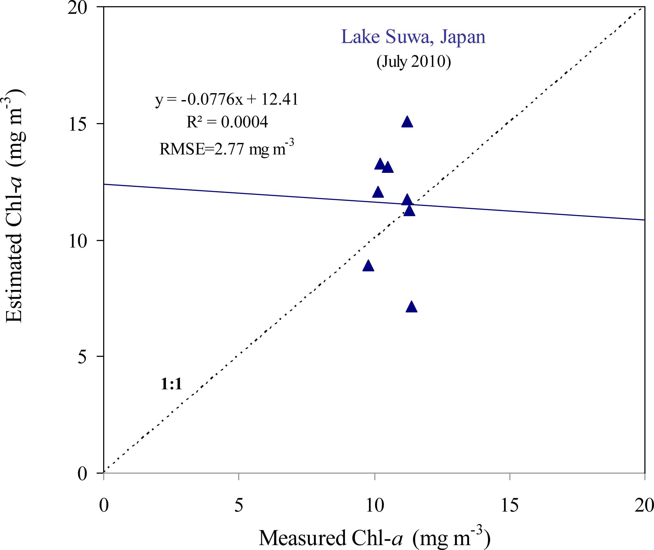
The second is Lake Suwa, which is located in the central part of Japan (36.05°N, 138.08°E, Nagano Prefecture). It has a surface area of 13.3 km², an average depth of 4.7 m, and a maximum depth of 7.2 m. In the 1960s, the lake underwent a very rapid hypertrophication. This was caused by the spectacular growth of industrial activity around the lake, and is indicated by heavy blooms of blue-green algae. Water quality has been remarkably improved since the end of 1990s, thanks to effective management. Therefore, the current trophic status of the lake is close to the boundary between mesotrophic and eutrophic.

The third lake is Lake Kasumigarua, situated in the eastern part of Japan’s Kanto plain (36.03°N, 140.40°E, Ibaraki Prefecture). It is Japan’s second largest lake, with a surface area of 171 km², an average depth of 4 m, and a maximum depth of 7.3 m (only for Nishiura). This lake is considered hypertrophic because of its high loads of nutrients and shallow depth [13]. Although average Chl-a has decreased from 87 to 61 mg·m⁻³ during the past three decades, the mean total phosphorus concentration increased from 116 to 138 mg·m⁻³. Secchi disk depth decreased from 70 to 52 cm in the last twenty years [14]. Total suspended sediment (TSS) concentrations increased from 14.1 to 26.4 g·m⁻³ during the last decade, due mainly to the resuspension of bottom sediments [15]. Diatoms (e.g., Cyclotella sp. or Synedra sp.) are generally observed during winter, spring, and autumn, while harmful blooms (blue green algae, e.g., Microcystis sp. or Anabaena sp.) are sometime observed during summer. The concentration of dissolved organic carbon (DOC), which is often correlated with CDOM concentration, is always low (2.9–4.2 g·m⁻³; [13,16]) compared to lakes such as Lake Taihu (8.8–20.2 g·m⁻³ in [17]) and Finnish lakes (6.0–12.3 g·m⁻³ in [18]). The absorption coefficients of CDOM at 420 nm ranged from 0.5 to 0.6 m⁻¹ when DOC concentrations ranged from 1.9 to 2.7 g·m⁻³ [14], which was lower than the absorption coefficients of CDOM at 420 nm in Finnish lakes (1.7–7.7 m⁻¹; [18]).

The fourth lake in our database is Lake Dianchi, located in a plateau area of the southwestern part of China (24.83°N, 102.72°E). It has a surface area of 300 km² and is the largest lake in Yunnan Province, with an average depth of 4.3 m, and a maximum depth of 11.3 m. Eutrophication has become more and more serious in the lake over the past 20 years due to the large quantities of industrial wastewater and municipal sewage discharged into it. Algal blooms occur frequently from April to November each year [19]. The trophic status of Lake Dianchi also belongs to the hypertrophic category.

The fifth and final lake is Lake Erhai (25.82°N, 100.18°E), which is the second largest lake in the Yunnan Province of China. It has a surface area of 249 km², an average depth of 11 m, and a maximum depth of 21 m. Lake Erhai is an important drinking water resource for the local people, supplying drinking water of 8.3 × 10⁴ m³ per day. It is also utilized for local industries, irrigation, and domestic water in the coastal area. During the past 30 years of rapid economic development and increasing population, Lake Erhai has faced a serious threat of intensive eutrophication due to anthropogenic inputs and overuse [20]. The water quality status of Lake Erhai is already at the initial stage of eutrophication, with organic matter and phytoplankton biomass increasing rapidly, and cyanobacteria blooms breaking out in the embayment and some parts of the lake.

3. Materials and Methods

3.1. Data Collection

Water samples and corresponding reflectance spectra were collected from Lake Biwa in a campaign undertaken in October 2011 (10 sites available); from Lake Suwa in a campaign in July 2010 (8 sites); from Lake Kasumigaura in February 2006, August 2008, and May 2010 (46 sites). Data collection was also carried out in Lake Dianchi in October 2007, July 2008, and July 2009 (28 sites). In Lake Erhai, there were two field campaign—one in September 2011 and the other in July 2012. In each field campaign, the investigation was performed at 21 sites (42 sites in total).

Reflectance was measured between 10:00 and 14:00 local time. All measurements were taken over optically deep water with depths larger than Secchi disk depth; floating scum was not found at these sampling sites. The water-leaving radiance (L_u(λ)), the downward irradiance (E_d(λ)), and the downward radiance of skylight (L_sky(λ)) were measured at each site using a FieldSpec HandHeld spectroradiometer (Analytical Spectral Devices, Inc., Boulder, CO, USA) in the range of 325 to 1075 nm at 1-nm intervals. The above-water remote-sensing reflectance (R_rs(λ)) was calculated approximately using the following equation [21]:

$$R_{\mathit{rs}}\approx \left(\frac{L_u(\lambda )}{E_d(\lambda )}-\frac{r{L}_{\mathit{sky}}(\lambda )}{E_d(\lambda )}\right)\times \mathit{Cal}(\lambda )\times 100$$

(1)

where Cal(λ) is the spectral reflectance calibration factor for the Spectralon reflectance panel, and r is the reflectance of skylight determined as a function of wind speed [21].

Water samples were collected at each site, and taken to laboratory within approximately 0.5–1.5 h after the field investigation. Chlorophyll-a was extracted using methanol (100%) at 4 °C for 24 h under dark conditions. The absorbance of the extracted chlorophyll-a was measured at four wavelengths (750, 663, 645 and 630 nm), and the concentrations were calculated according to SCOR-UNESCO equations [22]. The concentrations of total suspended solids (TSS), organic suspended solids (OSS), and inorganic suspended solids (ISS) were determined gravimetrically. Samples were filtered through pre-combusted Whatman GF/F filters at 500 °C for 4 h to remove dissolved organic matter in suspension, and then dried at 105 °C for 4 h and weighed to obtain TSS. The filters were re-combusted at 500 °C for 4 h and then weighed again to obtain ISS. OSS was derived by subtracting ISS from TSS. The absorption coefficient of CDOM was measured using a Shimadzu UV-2450 spectrophotometer after the water sample was filtered. The absorption coefficients of phytoplankton (a_ph) were measured according to the quantitative filter technique [23]. The a_ph data were available only for the stations collected after 2009.

3.2. SAMO-LUT Method

The basic idea of the SAMO-LUT involves the use of an imaginary case II body of water, in which only one constituent changes while the other two are controlled as constants [11]. A comprehensive synthetic dataset was used for model calibration, rather than in situ data. In this way, we hoped to obtain not only a large number of samples without a sampling bias for model calibration, but also a series of special cases to avoid effects from other constituents and thus improve model performance (e.g., a dataset only with various Chl-a while concentrations of NAP and CDOM are constants).

The procedures of the SAMO-LUT are summarized as follows:

• Step 1: Generation of simulation dataset. The R_rs spectra were generated based on the SIOPs from target water and a bio-optical model. In the present study, only the SIOPs collected from Lake Dianchi were used due to the lack of complete SIOPs data for other lakes. We felt it would be worthwhile to examine how the SIOPs affected the accuracy of the SAMO-LUT algorithm. The concentrations of Chl-a and NAP (i.e., tripton in the original paper), as well as the absorption coefficient of CDOM at 440 nm were varied in a wide range of 1–300 mg·m⁻³ (31 values), 1–250 g·m⁻³ (28 values) and 0.1–10 m⁻¹ (23 values), respectively. In all, 19,964 sample spectra were generated [11].
• Step 2: Computation of selected semi-analytical indices. Three semi-analytical indices were selected for the estimation of Chl-a, NAP and CDOM, based on their reasonableness and performance. The selected indices were: a three-band index ([1/R_rs(665) − 1/R_rs(708)]*R_rs(753)) for Chl-a, remote-sensing reflectance for the band centered 753 nm, R_rs(753), for NAP, and the band-ratio R_rs(560)/R_rs(665) for CDOM ([2,24]). The synthetic reflectances were resampled to the bandwidths of the MERIS (Medium Resolution Imaging Spectrometer) sensor based on its spectral response function, and then calculated as the selected indices.
• Step 3: Construction of look-up tables. We constructed three 2-dimensional look-up tables containing the coefficients of the estimation model for one constituent of interest, determined by the concentrations of the other two constituents. For instance, for the estimation of Chl-a, increments of 1 mg·m⁻³ for NAP and of 0.1 m⁻¹ for CDOM were respectively used in the ranges of 1–250 mg·m⁻³ and 0.1–10 m⁻¹, and the regression coefficients corresponding to different combinations of NAP and CDOM were stored in the LUT.
• Step 4: Initial estimations of Chl-a and NAP. We derived initial values of Chl-a and NAP using two general estimation models obtained through regression analysis between the simulated reflectance and corresponding Chl-a and NAP. The two general estimation models were:

  $$\text{Ch}1-a=223.86\left(R_{\text{rs},665}^{-1}-R_{\text{rs},708}^{-1}\right)\times R_{\text{rs},753}+23.95$$

  (2)

  $$\mathit{NAP}=49909R_{\text{rs},753}^2-61.38R_{\text{rs},753}+4.74$$

  (3)
  The calculated initial Chl-a and NAP were then used to estimate initial CDOM through a prepared LUT in Step 3.
• Step 5: Iteration to select more appropriate model coefficients. The estimation models were improved according to the initial Chl-a, NAP, and CDOM. After that, the refined Chl-a, NAP, and CDOM were obtained by using the improved estimation models.
• Step 6: End of iteration. We found a more appropriate estimation model from the LUTs for each water constituent through the iterative use of the newly obtained Chl-a, NAP and CDOM. The iteration was stopped when the difference between the current and last output was sufficiently small. Generally, the differences become stable after the 10th iteration.

3.3. Conventional 3-Band Index-Based Estimation Model

For comparison analysis, a conventional 3-band index-based linear model (Simple 3-band Model), calibrated by the same simulated dataset used in the SAMO-LUT, was also applied to the validation datasets ([11]). This model was used as the initial estimation of Chl-a in the SAMO-LUT method (i.e., Equation (2)). The comparison between this method and the SAMO-LUT can demonstrate how the iteration process in the SAMO-LUT method influences the estimation of Chl-a. In addition, it is worth noting that the slope and intercept of this linear model were close to those of the models proposed by the previous studies (e.g., 232.29 for slope and 23.174 for intercept in [9]).

3.4. Accuracy Assessment

Four indices (i.e., the root mean square error [RMSE], normalized root mean square error [NRMS], mean normalized bias [MNB], and normalized mean absolute error [NMAE]) were used in accuracy assessment [2,8]. These indices are defined as follows:

$$\text{RMSE}=\sqrt{\frac{\sum _{\text{i}=1}^N{\left({\text{X}}_{\text{esti},\text{i}}-{\text{X}}_{\text{meas},\text{i}}\right)}^2}{N-1}}$$

(4)

$$\text{NRMS}=\text{stdev}\left({\varepsilon }_{\text{i}}\right)\%$$

(5)

$$\text{MNB}=\text{mean}\left({\varepsilon }_{\text{i}}\right)\%$$

(6)

$$\text{NMAE}=\text{mean}\left(\left|{\varepsilon }_{\text{i}}\right|\right)\%$$

(7)

where X_esti,i and X_meas,i are the estimated and measured Chl-a, respectively; N is the number of samples; and ɛ_i = 100 × (X_esti,i − X_meas,i)/X_meas,i is the percent difference between the estimated and measured Chl-a. The NRMS denotes the relative random uncertainty of the results, the MNB denotes the average bias in the estimation, and the NMAE denotes the average relative error in the estimation. The correlation between the measured and estimated values was also calculated.

4. Results

4.1. Water Constituent Concentrations and Spectral Reflectance Properties

Table 1. Statistical description of water constituent concentrations for Lakes Biwa, Suwa, Erhai, Kasumigaura and Dianchi.

		Chl-a (mg·m−3)	TSS (g·m−3)	ISS (g·m−3)	OSS (g·m−3)	CDOM (m−1)
Biwa	Min	1.81	0.77	0.45	0.31	0.15
	Max	2.90	1.99	1.49	0.49	0.26
	Mean	2.21	1.01	0.64	0.38	0.21
	Median	2.02	0.87	0.55	0.34	0.20
	Stdev	0.43	0.37	0.31	0.07	0.03
	CV	19.33	36.61	49.24	19.33	15.64
Suwa	Min	9.79	4.81	1.21	3.30	0.41
	Max	11.37	6.06	2.19	4.79	0.48
	Mean	10.72	5.37	1.65	3.72	0.44
	Median	10.86	5.42	1.56	3.59	0.44
	Stdev	0.63	0.43	0.40	0.45	0.02
	CV	5.87	8.02	24.37	12.12	5.38
Erhai	Min	9.68	3.54	0.17	2.87	0.33
	Max	36.08	11.29	1.62	10.63	0.56
	Mean	19.58	5.75	0.78	4.98	0.41
	Median	18.73	5.64	0.83	5.08	0.40
	Stdev	5.92	1.70	0.40	1.61	0.06
	CV	30.20	29.45	51.51	32.30	13.49
Kasumigaura	Min	36.60	11.65	3.10	4.39	0.51
	Max	95.02	47.90	37.30	11.70	1.78
	Mean	66.47	24.45	16.31	8.13	0.90
	Median	67.88	21.92	14.50	8.42	0.92
	Stdev	19.48	8.24	7.28	2.36	0.29
	CV	29.30	33.70	44.65	29.03	32.04
Dianchi	Min	30.21	24.50	0.50	4.47	0.41
	Max	153.92	55.00	42.27	46.50	3.98
	Mean	87.74	37.38	12.39	24.98	1.25
	Median	84.56	37.42	6.50	27.00	0.96
	Stdev	29.16	7.80	11.79	11.49	0.84
	CV	33.23	20.86	95.12	46.01	66.87

contains descriptive statistics of the water constituent concentrations for the five lakes. Lake Biwa was the clearest, with mean Chl-a and TSS concentrations of 2.2 mg·m⁻³ and 1.0 g·m⁻³, respectively, followed by Lake Suwa (mean Chl-a of 11.4 mg·m⁻³ and mean TSS of 5.4 g·m⁻³), Lake Erhai (mean Chl-a of 19.6 mg·m⁻³ and mean TSS of 5.8 g·m⁻³), and Lake Kasumigaura (mean Chl-a of 66.5 mg·m⁻³ and mean TSS of 24.5 g·m⁻³). Lake Dianchi had the highest turbidity, with mean Chl-a and TSS concentrations of 87.7 mg·m⁻³ and 37.4 g·m⁻³, respectively. All five lakes showed low absorption coefficients of CDOM at 440 nm, with measures ranging from 0.15–3.98 m⁻¹ (most were less than 1 m⁻¹). The overall Chl-a of the five lakes varied by two orders of magnitude in the range of 1.8–153.9 mg·m⁻³. Except for Lake Suwa, each lake showed larger spatial heterogeneity for Chl-a (coefficient of variation larger than 19.3%). These datasets encompassed varying optical conditions and trophic statuses (from oligotrophic to hypertrophic), and thus can provide a thorough assessment of the SAMO-LUT method.

The reflectance spectra collected from the five lakes are shown in Figure 2. The reflectance spectra of Lake Biwa were similar to those collected from European lakes with low Chl-a and TSS (e.g., [25]), showing a unique peak in the green wavelength range (500–600 nm) and low magnitudes of the remote sensing reflectances along the visible and NIR spectral ranges (below 0.007 sr⁻¹). For the other four lakes, reflectance in the blue wavelength range (400–500 nm) was remarkably lower than in the green wavelength range (500–600) due to the high absorptions of phytoplankton, NAP, and CDOM in the shorter wavelengths (e.g., [3,4,8]). Reflectance troughs around 620 nm can be seen in the reflectance spectra of Lakes Erhai, Kasumigaura and Dianchi, demonstrating the dominance of cyanobacteria in those bodies of water [26]. A second minimum was also found at around 675 nm, which corresponded to the red Chl-a absorption maximum. In addition to chlorophyll, the reflectance near 675 nm was also affected by absorption and scattering by other constituents. A noticeable peak between 690 and 715 nm appeared in almost all spectra of the lakes except for Lake Biwa. This peak was the result of both high backscattering and a minimum in the absorption of all water constituents, including pure water [27,28]. Finally, reflectance in the NIR region (700–750 nm) varied widely, and was consistently comparable with that in the blue region. In the NIR region of the spectrum, reflectance is mostly controlled by the scattering of particulate matters.

4.2. Performance of the SAMO-LUT Algorithm for Each Lake

Figure 3 shows the comparison between the measured Chl-a and that estimated by the SAMO-LUT method for Lake Dianchi, China. The SAMO-LUT yielded an estimation of very high accuracy, with RMSE, NRMS, MNB and NMAE of 7.39 mg·m⁻³, 11.3%, 1.3% and 6.9%, respectively (

Table 2. Performance of the SAMO-LUT, Simple 3-band Model and OC4E for the estimation of Chl-a in Lake Dianchi, China.

	RMSE (mg·m−3)	NRMS(%)	MNB(%)	NMAE(%)	R2	Slope
Lake Dianchi, China (N = 28)
SAMO-LUT	7.39	11.3	1.3	6.9	0.94	0.998
Simple 3-band model	8.81	13.73	3.08	8.04	0.91	0.931
OC4E	79.14	8.7	−81.3	81.3	0.05	0.049

). It is worth noting that the dataset for Dianchi was collected over three years, and that the accuracy for each year was comparable with the data points distributed around the 1:1 line (Figure 3).

As for Lake Kasumigaura, Japan, and Lake Erhai, China, the SAMO-LUT was able to estimate the Chl-a with acceptable accuracy (Figures 4 and 5); NRMS, MNB and NMAE were lower than 22%, 4% and 18%, respectively (

Table 3. Performance of the SAMO-LUT, Simple 3-band Model and OC4E for the estimation of Chl-a in Lake Kasumigaura, Japan.

	RMSE (mg·m−3)	NRMS(%)	MNB(%)	NMAE(%)	R2	Slope
Lake Kasumigaura, Japan (N = 46)
SAMO-LUT	13.26	18.4	−3.9	16.2	0.64	0.511
Simple 3-band model	14.51	23.0	18.4	23.3	0.63	0.551
OC4E	59.60	13.1	−78.8	78.8	0.50	−0.143

and

Table 4. Performance of the SAMO-LUT, Simple 3-band Model and OC4E for the estimation of Chl-a in Lake Erhai, China.

	RMSE (mg·m−3)	NRMS(%)	MNB(%)	NMAE(%)	R2	Slope
Lake Erhai, China (N = 42)
SAMO-LUT	3.88	21.2	−2.8	17.1	0.71	1.025
Simple 3-band model	5.67	30.3	−19.4	26.6	0.74	1.306
OC4E	12.28	18.4	−50.1	50.3	0.01	0.047

). The high turbidity of the two lakes guaranteed that the SAMO-LUT method would be applicable to the reflectance at NIR-red wavelength. However, the accuracy of the estimates for these two lakes was noticeably lower than that for Lake Dianchi. This was because the SAMO-LUT was calibrated by the SIOPs of lake Dianchi, which likely differed from those for lakes Kasumigaura and Erhai.

Figure 6 shows the comparison between the measured and estimated Chl-a by SAMO-LUT for Lake Suwa. Compared with Lakes Kasumigaura and Erhai, the accuracy of SAMO-LUT was further reduced, with increasing NRMS, MNB and NMAE values of 23.9%, 8.3% and 19.8%, respectively (

Table 5. Performance of the SAMO-LUT, Simple 3-band Model and OC4E for the estimation of Chl-a in Lake Suwa, Japan.

	RMSE (mg·m−3)	NRMS(%)	MNB(%)	NMAE(%)	R2	Slope
Lake Suwa, Japan (N = 8)
SAMO-LUT	2.77	23.9	8.3	19.8	0.0004	−0.078
Simple 3-band model	4.72	32.2	−31.3	33.5	0.0007	0.147
OC4E	1.73	15.6	−1.0	12.2	0.0033	0.151

). Moreover, the correlation between measured and estimated Chl-a was statistically insignificant with very low R², which was probably due to the small dynamic range of Chl-a. It should be noted that the R² is shown here just for reference, but not for accuracy assessment. The reduced performance of SAMO-LUT in Lake Suwa was due to the decreased signal-to-noise ratio (SNR) at the NIR-red spectral regions owing to the low concentrations of phytoplankton and TSS (Table 1).

Figure 7 shows the comparison between the measured and estimated Chl-a in Lake Biwa by the SAMO-LUT method. Results showed that the SAMO-LUT yielded very large errors in this lake (see

Table 6. Performance of the SAMO-LUT, Simple 3-band Model and OC4E for the estimation of Chl-a in Lake Suwa, Japan.

	RMSE (mg·m−3)	NRMS(%)	MNB(%)	NMAE(%)	R2	Slope
Lake Biwa, Japan (N = 10)
SAMO-LUT	5.90	141.5	221.8	221.8	0.07	1.953
Simple 3-band model	20.84	276.83	−917.58	917.58	0.11	−4.39
OC4E	0.30	12.3	−1.1	9.4	0.54	0.592

, RMSE = 5.9 mg m⁻³, NRMS = 141.5%, and MNB = 221.8%). The very weak correlation between the estimated and measured Chl-a (R² = 0.07) indicated that the Chl-a estimated by SAMO-LUT could not explain actual Chl-a variation in Lake Biwa. This was because the concentrations of water constituents in the Lake Biwa were very low, and thus could not provide enough SNR for water-leaving reflectances at NIR-red spectral regions. This was despite the fact that, in theory, the SAMO-LUT can be used for such low concentrations [11].

4.3. Performance of the Simple 3-Band Model

The evaluation indexes for the Chl-a estimations using the Simple 3-band Model are also summarized in Tables 2 and 6. It can be seen that the Simple 3-band Model yielded remarkably lower accuracy for Lake Dianchi compared with the SAMO-LUT algorithm, with RMSE, NRMS, MNB and NMAE increased from 7.39 mg/m³, 11.3%, 1.3% and 6.9% to 8.81 mg/m³, 13.73%, 3.08% and 8.04%, respectively (Table 2). For the other two turbid lakes, Kasumigaura and Erhai, the SAMO-LUT also significantly outperformed the Simple 3-band Model, with much lower values of NRMS, MNB and NAME (Tables 3 and 4). These results indicate that the iteration process based on the look-up tables used in the SAMO-LUT method can effectively improve Chl-a estimation for turbid lakes with adequately high SNR in the NIR-red spectral regions. For Lake Suwa, a water body with relatively low turbidity, the Simple 3-band Model yielded very low accuracy, with values of NRMS, MNB and NAME larger than 30% (Table 5). Especially in the case of Lake Biwa, a body of water with fairly low loads of suspended solids, the Simple 3-band Model generated negative estimations for Chl-a, and consequently very large values of RMSE, NRMS, MNB and NMAE (over 300%, as shown in Table 6). It demonstrated again that the NIR-red bands-based methods do not work well for relatively clear waters.

4.4. Application of a Blue-Green Algorithm to Clear Waters

Since the SAMO-LUT and the Simple 3-band Model both yielded high errors in estimating Chl-a in relatively clear lakes like Suwa and Biwa, we tested a blue-green algorithm (OC4E, [29]) for these two lakes. The OC4E has been widely used for estimating Chl-a in case-1 waters using water-leaving reflectances at blue-green spectral regions (443, 490, 520, and 565 nm).

Figure 8 shows the comparison between the measured and estimated Chl-a by the OC4E for Lakes Suwa and Biwa. In the case of Lake Suwa, the OC4E performed slightly better than the SAMO-LUT (Table 5, RMSE: 1.7 mg·m⁻³ vs. 2.8 mg·m⁻³; NRMS: 15.6% vs. 23.9%; MNB −1.0% vs. 8.3%). Neither SAMO-LUT nor OC4E showed a significant correlation between the estimated and measured Chl-a in the lake. This was because of the small Chl-a variation among the sites (Table 1, CV = 5.9%). In contrast, the OC4E algorithm promised an accurate Chl-a estimation in Lake Biwa with an RMSE of 0.3 mg·m⁻³ and NRMS of 12.3%, as well as a small bias in the estimation (MNB = −1.1%, Table 6). The OC4E also explained 54% of the Chl-a variation in Lake Biwa even though the data had a narrow dynamic range (Chl-a ranging from 1.81–2.90 mg·m⁻³). This was likely because the effects of NAP and CDOM at the blue-green spectral regions were negligible in Lake Biwa due to the lower concentrations of NAP and CDOM (Table 1). We also tested the performance of OC4E for turbid waters (i.e., Lakes Dianchi, Kasumigaura and Erhai). The accuracy evaluation indexes are summarized in Tables 2 and 4. The OC4E not only produced a large underestimation (MNB ranging from −50.1% to −81.3%), but also could not present Chl-a variation for these lakes (very low determination coefficients except for Lake Kasumigaura, which showed a higher negative correlation).

The above results were not surprising. Previous studies have pointed out that water-leaving reflectances at blue-green spectral regions are influenced not only by phytoplankton but also by NAP and CDOM, and thus the OC4E fails in turbid productive waters [1,2,8,9,11]. To reduce the effects of NAP and CDOM for Chl-a estimation, these previous studies suggested the use of water-leaving reflectances at the NIR-red spectral regions. The SAMO-LUT was specifically designed based on these spectral regions [11]. The high concentrations of TSS in these three lakes improved SNR in the NIR-red spectral regions, and thus promised accurate estimations for Chl-a.

5. Discussion

One advantage of the SAMO-LUT algorithm is that the model calibration process requires a minimum of field data [11]. In the SAMO-LUT, only the SIOPs of water constituents must be collected from the target water. After that, a comprehensive synthetic dataset is generated based on the obtained SIOPs and a bio-optical model; and the LUTs are constructed to save the coefficients of water constituent estimation models (e.g., Chl-a estimation models). Yang et al. suggested that the LUTs should be reconstructed if the SAMO-LUT algorithm was applied to a water body with different SIOPs [11]. In practice, the SIOPs do change according to the dominant phytoplankton species in water bodies. For example, the dominant phytoplankton species changed seasonally in Lake Kasumigaura [14]. Generally, Cyanophyceae is the dominant species during the summer season, while Bacillariphyceae is dominant from autumn to spring. Therefore, the SIOPs changed accordingly [30]. The dominant phytoplankton species in Lakes Erhai and Dianchi were Cyanophyceae during the field surveys [31].

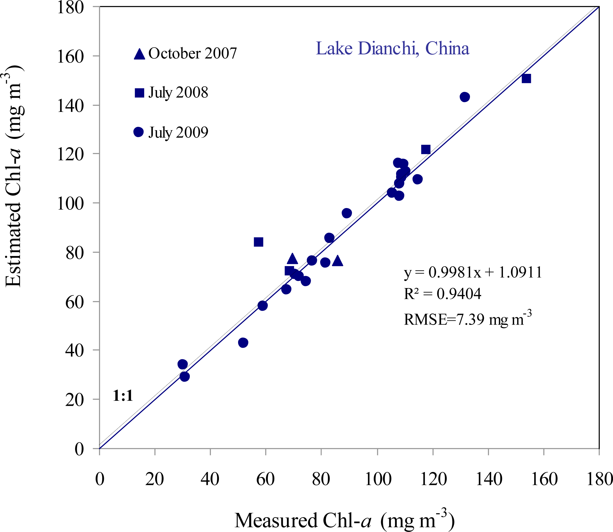
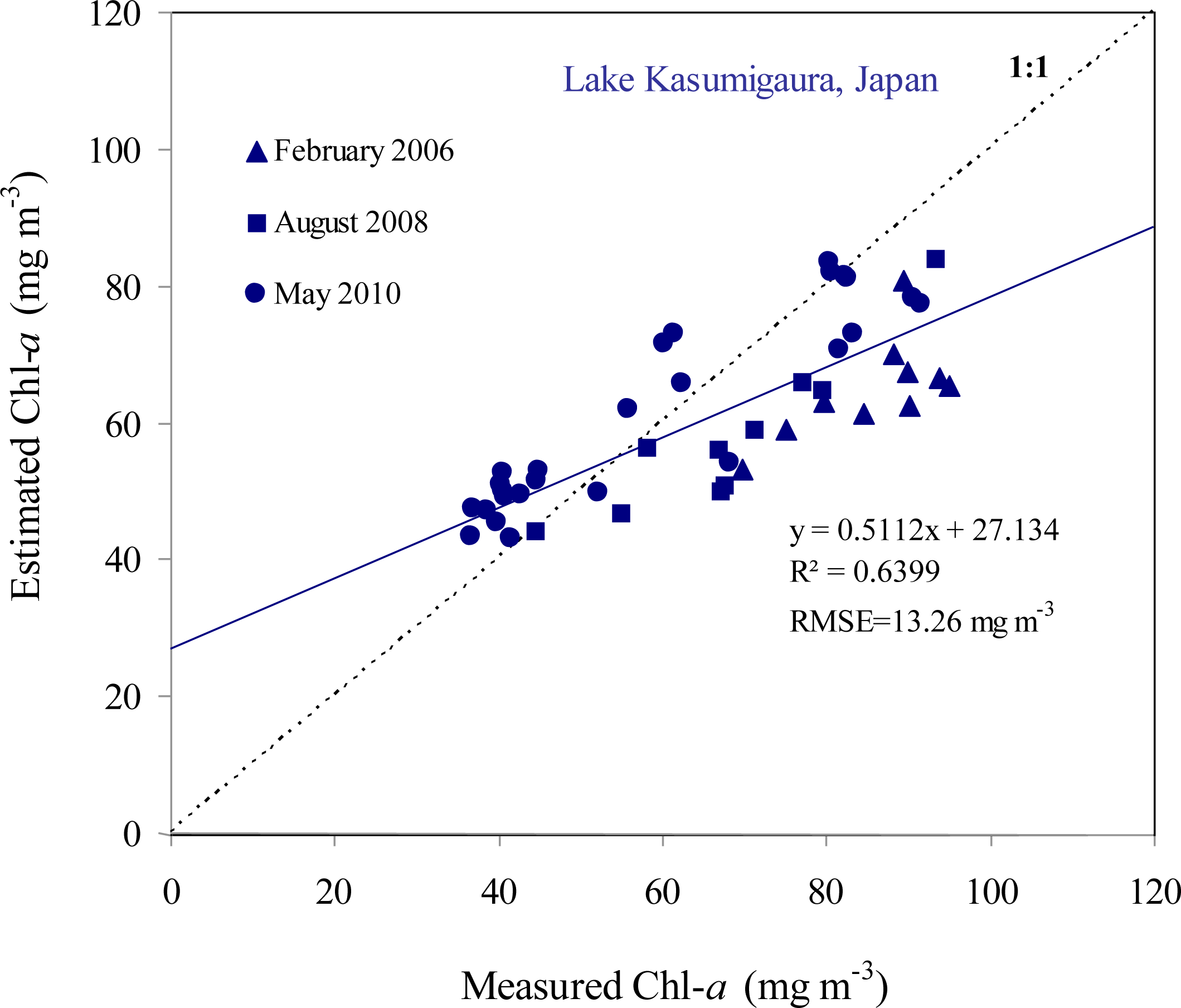
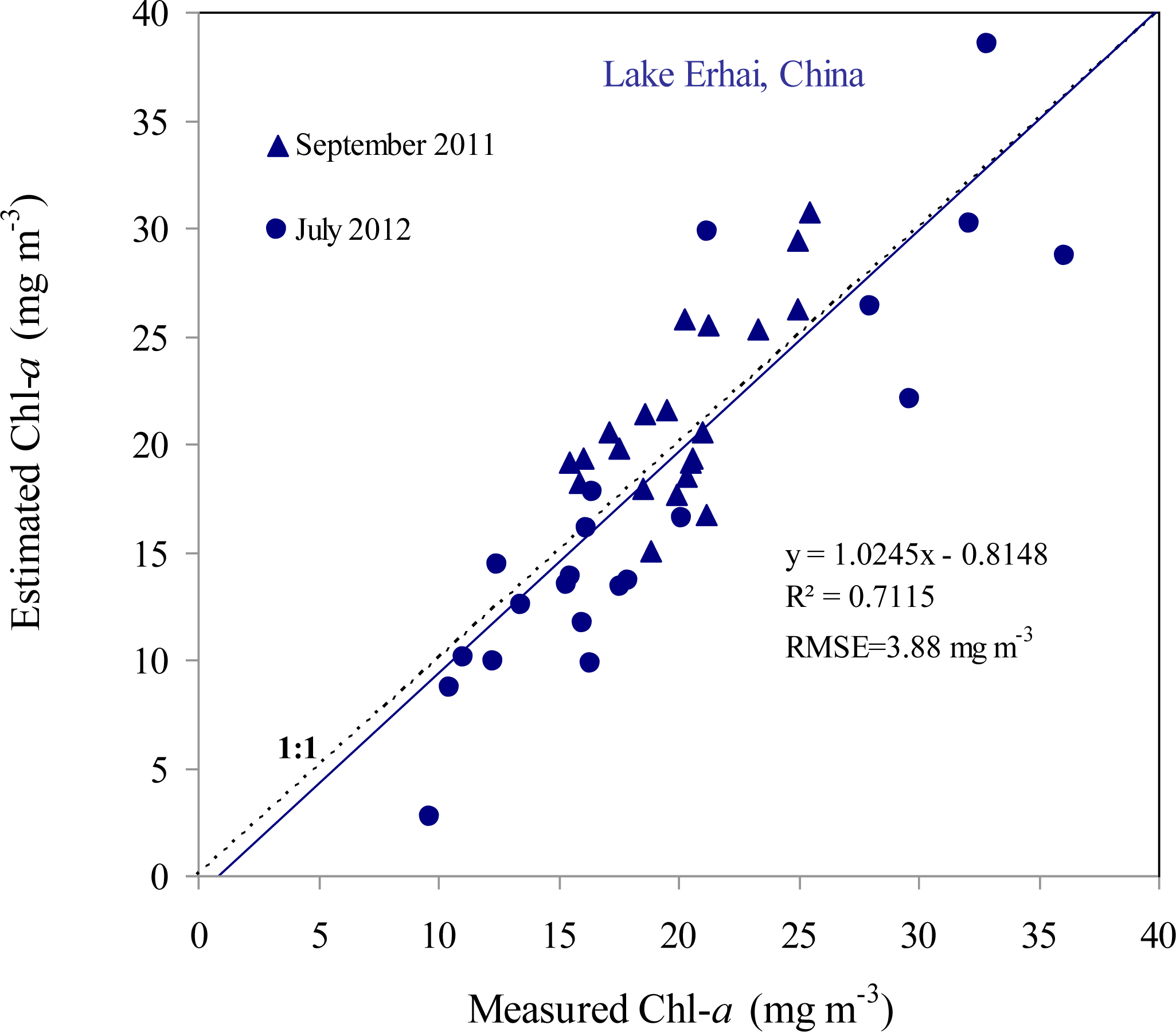
In this study, the SIOPs collected from Lake Dianchi in July 2009 were used to construct LUTs, which were then applied to other periods of Lake Dianchi and other lakes without any adjustment. The results in Section 4.2 showed that the SAMO-LUT algorithm was able to achieve acceptable accuracy for all tested cases, with NMAE less than 20%, except for Lake Biwa. These findings indicate that not only did the variation of SIOPs not affect the performance of the SAMO-LUT dramatically, but also that the use of a comprehensive synthetic dataset for model calibration can prevent the uncertainty in estimation models caused by sampling bias. Our results thus present a strong case for the use of the SAMO-LUT algorithm as an operational method for estimating Chl-a from remote sensing data. Moreover, the best performance of the SAMO-LUT algorithm in Lake Dianchi and its slightly degraded performance in Lake Kasumigaura in February 2006 suggest that the algorithm has the potential to provide more accurate Chl-a estimation if the SIOPs of the target water were available.

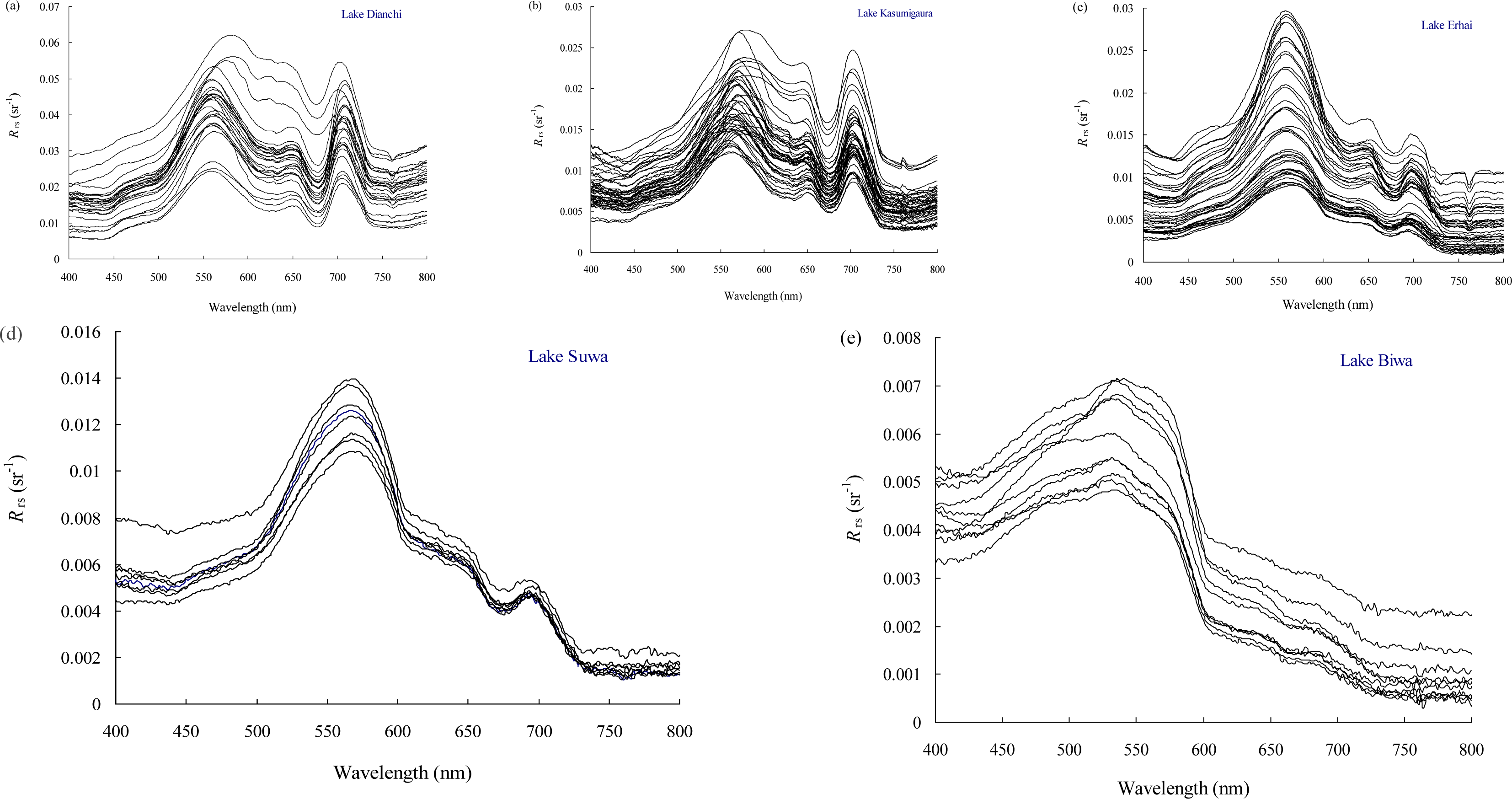
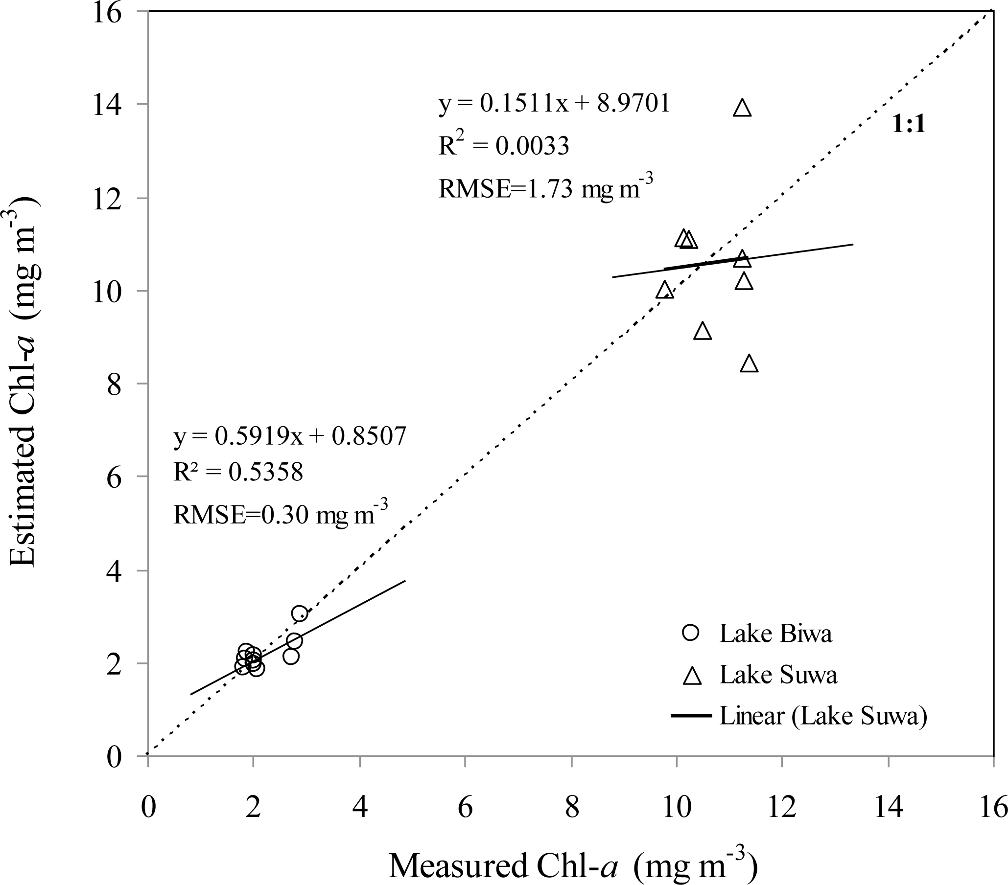
We do not believe, however, that the failure of the SAMO-LUT algorithm in the cases of Lakes Biwa and Suwa were caused by the differences in SIOPs between them and Lake Dianchi. In the other words, the performance of the SAMO-LUT algorithm would not have been satisfactorily improved had SIOPs been collected from these two lakes. From Figure 2 it can be seen that the R_rs in the red-NIR spectral region of Lakes Biwa and Suwa are much lower than those of the other three lakes. Weak signals from water bodies with too low TSS will be hidden by environmental noise, and thus cannot provide enough information for estimating water constituents. Therefore, the SNR at selected red-NIR bands used in the SAMO-LUT algorithm are not applicable to relatively clear waters. Alternatively, for clear waters with negligible effects of NAP and CDOM, a blue-green algorithm (e.g., OC4E) can be used to replace the NIR-red algorithms (e.g., Lakes Biwa and Suwa) because the signals in blue-green spectral regions remain strong even for this kind of water. A classification method for selecting an appropriate algorithm in the case of different types of water is needed.

On the other hand, the SAMO-LUT algorithm was developed based on the bandwidths of Mediun Resolution Imaging Spectrometer (MERIS). The most important prerequisite is the band around 708 nm, as used in the three-band index. Therefore, it can be directly applied to water-color sensors with configurations similar to MERIS, such as the Ocean and Land Color Instrument (OLCI, [32]), the Hyperspectral Infrared Imager (HyspIRI, [33]) or the Airborne Imaging Spectrometer for Applications (AISA, [5]). Extension of the SAMO-LUT method to more satellite sensors without the 708 nm band, such as the Moderate Resolution Imaging Spectroradiometer (MODIS), and the Sea-viewing Wide Field-of-view Sensor (SeaWiFS), will be carried out in future studies.

6. Conclusions

The performance of the Semi-Analytical Model Optimizing and Look-Up Table (SAMO-LUT), a recently developed algorithm for estimating Chl-a in inland waters, was evaluated using an extensive dataset collected from five Asian lakes in which the concentrations of total suspended solids varied from 0.77 to 55.00 g·m⁻³. Results showed that the SAMO-LUT algorithm was able to provide acceptably accurate estimates for all cases but one, with normalized mean absolute error (NMAE) less than 20% (the exception was Lake Biwa). This was the case even though the specific inherent optical properties (SIOPs) from Lake Dianchi were used for all lakes. These findings indicate that a variation in SIOPs does not significantly affect the performance of the SAMO-LUT algorithm, and thus it has the potential to be an operational method for estimating Chl-a from remote sensing data. The failure of the SAMO-LUT algorithm in the case of Lake Biwa (NMAE of 221.8%) was mainly to the lack of sufficient signals from water-leaving reflectances at the NIR-red spectral regions, due to very low concentrations of Total Suspended Solids in the water, rather than to the use of SIOPs from Lake Dianchi in the algorithm. To overcome this problem, a blue-green algorithm such as the OC4E could be used to replace the SAMO-LUT algorithm for estimating Chl-a concentration in Lake Biwa, which could reduce the NMAE to 9.4%. It is therefore necessary to develop a classification method in future for selecting the appropriate algorithm for different cases of waters.

References

1. Gilerson, A.A.; Gitelson, A.A.; Zhou, J.; Gurlin, D.; Moses, W.; Loannou, L.; Ahmed, S.A. Algorithms for remote estimation of chlorophyll-a in coastal and inland waters using red and near infrared bands. Opt. Express 2010, 18, 24109–24125. [Google Scholar]
2. Gitelson, A.A.; Dall’Olmo, G.; Moses, W.; Rundquist, D.C.; Barrow, T.; Fisher, T.R.; Gurlin, D.; Holz, J. A simple semi-analytical model for remote estimation of chlorophyll-a in turbid waters: Validation. Remote Sens. Environ 2008, 112, 3582–3593. [Google Scholar]
3. Gitelson, A.A.; Gurlin, D.; Moses, W.J.; Barrow, T. A bio-optical algorithm for the remote estimation of the chlorophyll-a concentration in case 2 waters. Environ. Res. Lett 2009, 4. [Google Scholar] [CrossRef]
4. Gons, H.J. Optical teledetection of chlorophyll a in turbid inland waters. Environ. Sci. Tech 1999, 33, 127–1132. [Google Scholar]
5. Moses, W.J.; Gitelson, A.A.; Perk, R.L.; Gurlin, D.; Rundquist, D.C.; Leavitt, B.C.; Barrow, T.M.; Brakhage, P. Estimation of chlorophyll-a concentration in turbid productive waters using airborne hyperspectral data. Water Res 2012, 46, 993–1004. [Google Scholar]
6. El-Alem, A.; Cholmani, K.; Laurion, I.; Eo-Adlouni, S. Comparative analysis of four models to estimate chlorophyll-a concentration in case-2 waters using Moderate Resolution Imaging Spectroradiometer (MODIS) imagery. Remote Sens 2012, 4, 2373–2400. [Google Scholar]
7. Dall’Olmo, G.; Gitelson, A.A.; Rundquist, D.C. Towards a unified approach for remote estimation of chlorophyll-a in both terrestrial vegetation and turbid productive waters. Geophy. Res. Lett 2003, 30. [Google Scholar] [CrossRef]
8. Gurlin, D.; Gitelson, A.A.; Moses, W.J. Remote estimation of Chl-a concentration in turbid productive waters—Return to a simple two-band NIR-red model? Remote Sens. Environ 2011, 115, 3479–3490. [Google Scholar]
9. Moses, W.J.; Gitelson, A.A.; Berdnikov, S.; Povazhnyy, V. Satellite estimation of chlorophyll-a concentration using the red and NIR bands of MERIS—The Azov sea case study. IEEE Geosci. Remote Sens. Lett 2009, 6, 845–849. [Google Scholar]
10. Le, C.; Li, Y.; Sun, D.; Huang, C.; Lu, H. A four-band semi-analytical model for estimating chlorophyll a in highly turbid lakes: The case of Taihu Lake, China. Remote Sens. Environ 2009, 113, 1175–1182. [Google Scholar]
11. Yang, W.; Matsushita, B.; Chen, J.; Fukushima, T. Estimating constituent concentrations in case II waters from MERIS satellite data by semi-analytical model optimizing and look-up tables. Remote Sens. Environ 2011, 115, 1247–1259. [Google Scholar] [Green Version]
12. Yang, W.; Matsushita, B.; Chen, J.; Fukushima, B.; Ma, R. An enhanced three-band index for estimating chlorophyll-a in turbid case-II waters: Case studies of Lake Kasumigaura, Japan, and Lake Dianchi, China. IEEE Geosci. Remote Sens. Lett 2010, 7, 655–659. [Google Scholar]
13. Fukushima, T.; Park, J.; Imai, A.; Matsushige, K. Dissolved organic carbon in a eutrophic lakes; dynamics, biodegradability and origin. Aquat. Sci. 1996, 58, 139–157. [Google Scholar]
14. CGER, Lake Kasumigaura Database; National Institute for Environmental Studies: Tsukuba, Japan, 2010.
15. Fukushima, T.; Kawamura, S.; Seki, T.; Onda, Y.; Imai, A.; Matsushige, K. Why has Lake Kasumigaura become turbid? In Verhandlungen. Verh. Int. Ver. Theor. Angew. Limnol 2005, 29, 732–737. [Google Scholar]
16. Imai, A.; Matsushige, K.; Nagai, T. Triharomethane formation potential of dissolved organic matter in a shallow eutrophic lake. Water Res 2003, 37, 4284–4294. [Google Scholar]
17. Zhang, Y.L.; Gin, B.Q; Chen, W.M.; Zhu, G.W. A preliminary study of chromophoric dissolved organic matter (CDOM) in Lake Taifu, a shallow subtropical lake in China. Acta Hydrochim. Hydrobiol 2005, 33, 315–323. [Google Scholar]
18. Kutser, T.; Piersion, D.C.; Kallio, K.Y.; Reinart, A.; Sobek, S. Mapping lake CDOM by satellite remote sensing. Remote Sens. Environ 2005, 94, 535–540. [Google Scholar]
19. Gao, L.; Zhou, J.M.; Yang, H.; Chen, J. Phosphorus fractions in sediment profiles and their potential contributions to eutrophication in Dianchi Lake. Environ. Geol 2005, 48, 835–844. [Google Scholar]
20. Zheng, G.; Fu, B.; Duan, Y.; Wang, Q.; Matsuo, M.; Takano, B. Iron speciation related to colors of Jurassic sedimentary rocks in Turban Basin, Northwestern China. J. Radioanalyt. Nucl. Chem 2004, 26, 421–427. [Google Scholar]
21. Mobley, C.D. Estimation of the remote-sensing reflectance from above-surface measurements. Appl. Opt 1999, 38, 7442–7455. [Google Scholar]
22. SCOR-UNESCO, Determination of Photosynthetic Pigment in Seawater. Monographs on Oceanographic Methodology; Imprimerie Rolland: Paris, France, 1966.
23. Mitchell, B.G. Algorithms for determining the absorption coefficient of aquatic particulates using the quantitative filter technique. Proc. SPIE 1990. [Google Scholar] [CrossRef]
24. Ammenberg, P.; Flink, P.; Lindell, T. Bio-optical modelling combined with remote sensing to assess water quality. Int. J. Remote Sens 2002, 23, 1621–1638. [Google Scholar]
25. Odermatt, D.; Giardino, C.; Heege, T. Chlorophyll retrieval with MERIS Case-2-Regional in perialpine lakes. Remote Sens. Environ 2010, 114, 607–617. [Google Scholar] [Green Version]
26. Simis, S.G.H.; Peters, S.W.M.; Gons, H.J. Remote sensing of the cyanobacterial pigment phycocyanin in turbid inland water. Limnol. Oceanogr 2005, 50, 237–245. [Google Scholar]
27. Gitelson, A.; Keydan, G.; Shishkin, V. Inland waters quality assessment from satellite data in visible range of the spectrum. Soviet Remote Sens 1985, 6, 28–36. [Google Scholar]
28. Gitelson, A.A. The peak near 700 nm on reflectance spectra of algae and water: Relationships of its magnitude and position with chlorophyll concentration. Internat. J. Remote Sens 1992, 13, 3367–3373. [Google Scholar]
29. O’Reilly, J.E.; Maritorena, S.; Mitchell, B.G.; Siegel, D.A.; Carder, K.L.; Garver, S. Ocean color chlorophyll algorithms for SeaWiFS. J. Geophys. Res 1998, 103, 24937–24953. [Google Scholar]
30. Yang, W.; Matsushita, B.; Chen, J.; Fukushima, T. A relaxed matrix inversion method for retrieving water constituent concentrations in case II waters: The case of Lake Kasumigaura, Japan. IEEE Trans. Geosci. Remote Sens 2011, 49, 3381–3392. [Google Scholar]
31. Wang, Z.; Wang, Y.; Hu, M.; Li, Y.; Liu, Y.; Shen, Y.; Li, G.; Wang, G. Succession of the phytoplankton community in response to environmental factors in north Lake Erhai during 2009–2010. Fresenius Environ. Bull 2011, 20, 2221–2231. [Google Scholar]
32. Donlon, C.; Berruti, B.; Buongiorno, A.; Ferreira, M.-H.; Féménias, P.; Frerick, J.; Goryl, P.; Klein, U.; Laur, H.; Mavrocordatos, C.; et al. The Global Monitoring for Environment and Security (GMES) Sentinel-3 mission. Remote Ses. Environ 2012, 120, 37–57. [Google Scholar]
33. Devred, E.; Turpie, K.R.; Moses, W.; Klemas, V.V.; Moisan, T.; Babin, M.; Toro-Farmer, G.; Forget, M.-H.; Jo, Y.-H. Future retrievals of water column bio-optical properties using the Hyperspectral Infrared Imager (HyspIRI). Remote Sens. 2013, 5, 6812–6837. [Google Scholar]
Figure 1. Distribution of sampling sites in Lakes Erhai and Dianchi of China; and Lakes Biwa, Suwa and Kasumigaura of Japan.
Remotesensing 06 03492f1
Figure 2. Remote-sensing reflectance collected from Lakes Biwa, Erhai, Suwa, Kasumigaura and Dianchi.
Remotesensing 06 03492f2
Figure 3. Comparison of the measured and estimated Chl-a by the SAMO-LUT for Lake Dianchi, China.
Remotesensing 06 03492f3
Figure 4. Comparison of the measured and estimated Chl-a by the SAMO-LUT for Lake Kasumigaura, Japan.
Remotesensing 06 03492f4
Figure 5. Comparison of the measured and estimated Chl-a by the SAMO-LUT for Lake Erhai, China.
Remotesensing 06 03492f5
Figure 6. Comparison of the measured and estimated Chl-a by the SAMO-LUT for Lake Suwa, Japan.
Remotesensing 06 03492f6
Figure 7. Comparison of the measured and estimated Chl-a by the SAMO-LUT for Lake Biwa, Japan.
Remotesensing 06 03492f7
Figure 8. Comparison of the measured and estimated Chl-a by the OC4E algorithm for Lakes Suwa and Biwa, Japan.
Remotesensing 06 03492f8