Change Detection of Tree Biomass with Terrestrial Laser Scanning and Quantitative Structure Modelling

 , and
, and
Abstract
: We present a new application of terrestrial laser scanning and mathematical modelling for the quantitative change detection of tree biomass, volume, and structure. We investigate the feasibility of the approach with two case studies on trees, assess the accuracy with laboratory reference measurements, and identify the main sources of error, and the ways to mitigate their effect on the results. We show that the changes in the tree branching structure can be reproduced with about ±10% accuracy. As the current biomass detection is based on destructive sampling, and the change detection is based on empirical models, our approach provides a non-destructive tool for monitoring important forest characteristics without laborious biomass sampling. The efficiency of the approach enables the repeating of these measurements over time for a large number of samples, providing a fast and effective means for monitoring forest growth, mortality, and biomass in 3D.1. Introduction
The monitoring of forest resources has traditionally concentrated on the volume of stem wood. This is because human interest in forests has strongly focused on this economically most valuable forest characteristic. Today, the importance of forests is seen in a wider perspective. It is acknowledged that several ecosystem services that forests provide are related to the whole biomass of trees rather than the stem only. These services include, for example, carbon sequestration, forest bioenergy resources and forest biodiversity value.
Tree biomass is monitored using established but rather coarse methods. A common method of biomass monitoring (such as that in the IPCC Guidelines [1]) is based on allometric equations (e.g., [1,2]). These equations give the biomass estimates as a function of stem characteristics, such as tree height and the diameter [3,4]. The same equations are also used to estimate changes in the biomass based on changes in the stem characteristics [1]. The mortality of tree biomass components is monitored using litter collectors placed below tree canopies or deriving estimates from canopy measurements (e.g., [5]). The litter production measurements are combined with the biomass estimates to obtain turnover rates of tree biomass components; the turnover rate is equal to the litter production divided by the biomass (e.g., [6]). These turnover rates are then used to estimate litter production based on the biomass estimates. Although these methods are practical, their reliability and usefulness can still be improved. First, the allometric equations and the biomass turnover rates can be made more reliable and applicable to new conditions by taking more measurements. Since the current allometric equations and biomass turnover rates are based on laborious biomass and litter measurements, they are still based on relatively small data sets that represent selected intensively studied sites. Second, these methods do not provide all the information needed for current and future analyses. For example, the size of litter elements is an important attribute affecting the decomposition of litter [7,8]. This information is thus relevant for the carbon budget of forests, but is very laborious to measure from the litter collectors. In addition, the distribution of the biomass within a canopy is a key characteristic in understanding the light-use efficiency and the competitive status of a tree [9]. The light-use efficiency (LUE); i.e., the amount of carbon fixed per unit of absorbed photosynthetically active radiation, increases with the proportion of light that is received at low irradiances and is therefore higher for clumped canopies [10]. Thus, fast measurements of the canopy branching pattern can help to predict the efficiency with which canopies harvest light for carbon assimilation. Since the LUE is frequently used with the remote-sensed Normalized Difference Vegetation Index (NDVI) to calculate productivity, methods that improve the understanding of the variation of the LUE are important to global carbon balance estimates [11].
Terrestrial laser scanning (TLS) has become increasingly important in forest studies because of its capability of providing accurate 3D tree data with efficient and lightweight instruments for field use. Thus far, TLS-based methods have been established for detecting forest attributes such as tree location, the diameter at breast height (DBH), height, stem volume, and the total biomass [12–14]. The total biomass has been shown to correlate with the TLS point density or distribution [13,15], DBH, and tree height, from which it is possible to retrieve with allometric biomass equations [3,4,16]. These methods provide the total biomass of a tree and a stand, without information on its distribution in the canopy. Tree modelling has thus far mostly focused on retrieving the stem volume for forest (timber) inventory purposes [17,18]. Quite recently, methods have also been presented for tree 3D structure including branches [19–21]. These studies have also extended into 3D reconstructions of the stump-root systems [22,23]. An error range of ±10% has been achieved for the main stem volume, whereas for branches, the cumulative branch volumes have been estimated at ±30% accuracy for branches down to 7 cm in diameter [20]. Increasing the number of scans has been shown to reduce the errors somewhat [21]. Getting quantitative structure models for trees with small branches has, however, still been a challenge, and the small branches have most often been excluded from the analysis. A plant topology model was presented in [24] to describe the topology and geometry of plants. They also recorded the spatial coordinates of plants (e.g., branch tips).
In our previous study, we have shown that the structure of trees can be characterized in detail based on TLS measurements combined with 3D quantitative structure modelling (which we hereafter call QSM) [25]. If these measurements and this modelling were repeated over time, it could potentially provide a largely automatic, non-destructive and fast means to estimate the growth and mortality of tree biomass components in 3D.
In our QSM of trees, we use the geometric primitives approach with circular cylinders. Alternative methods for modelling the tree volume based on voxels and voxel skeletons exist (e.g., [14,26,27]). While the voxel and skeletonization models have been used successfully for extracting tree metrics, such as the diameter and height [28], the QSM is different from these models because it has been designed to follow the simple morphological rules of tree structure (such as branches attached to the stem and sub-branches being attached to the main branches, cf. [25]) as a starting point for the calculation. A particular challenge in the voxel methods is that they require a complete sampling of the tree surface in order to fill the interior voxels. This requires a large number of measurements and scan positions (e.g., 20–60 million points from 4 to 5 scan positions per tree [28]). With cylinders, the inevitable gaps in the surface sampling and the fact that most branches are sampled only from the bottom side are not so critical. Similarly, the voxel skeleton models do not require a large number of measurements because the voxels are only needed for the reconstruction of the skeleton and then the volume is modelled, e.g., with cylinders [27]. Changes in the total biomass have been monitored with TLS and voxel or convex hull models [29], but more studies are needed to quantify the distribution of the changes.
The objectives of this study were to (1) evaluate the suitability of this approach (presented in [25]) for estimating changes in tree biomass, e.g., growth and litter production; and (2) identify the most important areas for improvement. The comparison with reference measurements also enabled us to improve the data processing and modelling steps to optimize the procedure by finding and eliminating the sources of major systematic errors in the measurement (e.g., removing extra noise) or modelling the smallest branch tips. In this way, we improved the procedure for more reliable results. The change detection approach presented in this paper is applied to free-standing trees. Our future objective is to extend the approach into large areas and to validate such plot-based modelling. We have used and will use the outputs of this procedure to compute carbon emissions via, e.g., the Yasso soil carbon model as in [23].
This article is organized as follows: the materials and methods are presented in Section 2. The results for both the laboratory and field cases are in Sections 3.1–3.3, and the discussion and conclusions are presented in Sections 3.4 and 4, respectively.
2. Materials and Methods
2.1. Samples
We demonstrate the approach with two case studies: the first one was carried out in a laboratory for a large (about 2 m in length) aspen (Populus tremula) branch. We created a time series of volume and length measurements by cutting off pieces of the sub-branches, after which the branch was scanned with a terrestrial laser scanner (see Section 2.2). The scanning was repeated four times (from three directions each time) and the cuts were carried out between each scan. The aim of these measurements was to provide reference to validate the branch size (the volume and length of the stem and all sub-branches) estimation with the QSM model.
The second case study was a field monitoring of changes in tree biomass in Espoonlahti, Finland. We produced a time series of TLS point clouds for a maple (Acer platanoides) shown in Figure 1. Five scans were carried out: in February 2011, November 2011, November 2012, April 2013, and November 2013. The changes in tree branch volume and branch length, caused by growth and mortality, were modelled from each point cloud.
2.2. Terrestrial Laser Scanning
Both the tree and the branch sample were measured with a phase-based terrestrial laser scanner Leica HDS6100, see Table 1 for scanner parameters. The same scanner (and the same scanning parameters) was also used in our previous studies [25]. The instrumental parameters related to each measurement are listed in Table 2. The scanning was carried out with the “High” resolution setup. To produce a point cloud, three stationary TLS scans were carried out for each sample from different directions, and these scans were co-registered using white spherical reference targets (visible in Figure 1 during the TLS of the Espoonlahti maple, cf. [13]). The co-registration accuracy is best described in terms of the error in locating the centre points of the spherical reference targets, which varied between 1 and 3 mm in the laboratory. However, there are greater sources of uncertainty, especially in outdoor measurements, caused by, e.g., the branches moving during the scans. In Espoonlahti, some parts of the target (such as the canopy) were further from the scanner, and the co-registration accuracy varied from 4 to 7 mm. The distance between the scanner and the tree varied from 1 to 2 m in the laboratory and 9–20 m in Espoonlahti. The aspen branch was scanned before any cuts and after each three cuts, from three different directions each time. After the third cut, we carried out two independent scans (denoted with cut 3A and 3B in the following sections), i.e., altogether six scans were made. This was done to compare the repeatability of the measurement and modelling procedures.
The pre-processing of the TLS data was carried out with the Z+F LaserControl 8 software (Zoller + Fröhlich GmbH). The distance measurement of the scanner, based on phase difference, causes increased mixed pixel noise in complex structures, where the laser beam hits multiple targets at the same time. The measurement noise was minimized with intensity- and point-density based filters available with the Z+F software. In this case, noise filtering resulted in the rejection of 1%–3% of the data points.
2.3. Reference Measurements
To change the branch length and volume in the laboratory, the sample branches of the aspen were cut after each measurement of point clouds. The lengths of the cut branch pieces were measured manually (with a standard metric measure). The total volume removed in each cut was measured by weighing the cut branches, and approximating their volume on the basis of their density. The density of the fresh sample branches was measured by submerging the branch pieces in water and recording the increase of weight of the water replaced by the branches. The weight represents the volume, and the fresh weight divided by this volume gives the density, which was used as a density approximation for the entire branch. In this way, the approximate fresh density for our sample branches was 0.925 kg/dm3. We also measured the total length and volume of the entire branch (including all the sub-branches) after the third cut of branches (after which we made two sets of scans, which were processed as two independent three-scan measurements, 3A and 3B). Because the total volume reference was retrieved using the approximate density measured from small branch bits, some uncertainty may occur in the density of the larger parts of the branch. These branch length and volume values were compared to those produced by TLS and the QSM model [25].
2.4. Quantitative Structure Modelling (QSM)
The branch size and volume for each sample was computed using the quantitative structure modelling method [25]. In the QSM, the surface of the visible tree parts is reconstructed by making a flexible surface model of the tree to model the stem and branch sizes and the topological branching structure. The method uses a local approach in which the point cloud is covered with small sets corresponding to connected surface patches in the tree surface. With these patches the entire tree is segmented into stem and branches. The patches are randomly but evenly distributed along the visible tree surface and their size determines the smallest details that can be separated for the tree model. The segments are then modelled with collection of cylinders fitted to the details of the segments. With these cylinders, the branching structure, volume, and branch size distributions, etc. can be approximated both for the whole tree and some of its parts individually. We use cylinders because of all the geometric primitives that approximate the local stem and branch shape well, they are the most robust and reliable to fit. More details of the model and its validation are provided in [25].
We also compared the QSM with the Triangulated Irregular Network (TIN), commonly used for filtering laser scanner data for digital elevation model (DEM) generation and producing 3D models of different objects [30,31].
The TIN model was a reduced 3D Delaunay triangulation. The algorithm had the following steps:
The raw point cloud was first triangulated with 3D Delaunay triangulation.
Tetrahedrons with side lengths over a predefined threshold (3 cm) were removed.
The surface of the reduced triangulation was searched and then divided into separate layers using points on the surface as initial points.
The second tetrahedron reduction run with 2 cm threshold was carried out for the tetrahedrons in the two outermost layers.
The tree volume was estimated by summing the volume of the tetrahedrons remaining after both reduction runs.
No additional smoothing was done for the point clouds, thus some noise points near branches and the stem were left, resulting in overestimation of the tree volume.
3. Results and Discussion
3.1. Aspen Branch Measured in Laboratory: Validation of Branch Size Modelling
The changes in the volume (Table 3) and length (Table 4) of branches estimated with the QSM agreed well with reference measurements. The modelling was carried out as if the branch were a small tree, i.e., the main branch was segmented as “stem”, whereas the sub-branches are treated as branches. All changes are mean values of 10 modelling runs, where the size of the average patch remains constant but their number and locations vary randomly between different models which affects the segmentation and fitted cylinders. Typical ranges of the standard deviations of the 10 models of each cut are 5%–15% for the branch volume and 1%–2% for the branch length.
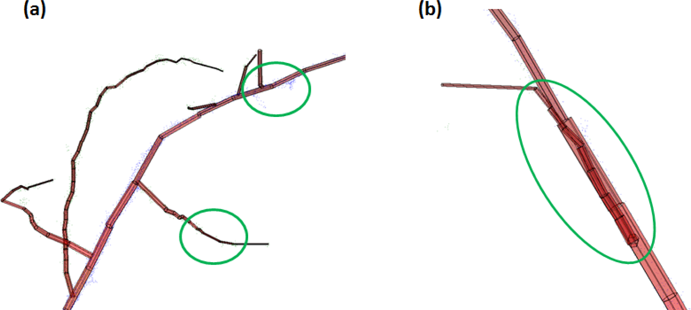
The point clouds and models are presented in Figures 2 and 3. To compare with the reference measurements, which were carried out for the cut pieces only, the modelling results are also presented here as changes from the original condition of the branch (before any cuts). The model has underestimated the cumulative changes, which is most likely a result of inaccuracies in the measurement; see Section 3.2 for more details. A close examination of the point clouds and models (see Figure 4) revealed that the smallest sub-branches (those with length less than 5 cm) were hardly visible in the point cloud, and had mostly been left out by the model. The number of points for those bits is too small to form a cylinder. To get some insight into the effect of this feature on the results, we made another length reference, where the smallest (<5 cm) sub-branches had also been omitted (see Table 4). In addition, some segmentation errors were also present, resulting in the cylinders overlapping each other (Figure 4). A further analysis on the overall accuracy of the approach is provided in Section 3.2.
The QSM and TIN models are compared in Figure 5, which also presents the standard deviation errors for the QSM. In the initial tests, both models overestimated the branch volume change by several orders of magnitude. This results from the inaccuracy in measurement, because the diameters of the branch tips are less than or equal to the laser spot size (about 3 mm) towards the branch tips. Therefore, we used a modified approach to the QSM presented in [25], where the sizes of branches with diameter less than 1 cm were approximated with a branch diameter that decreases linearly towards the branch end. This improved the results, although some discrepancy between the measurements and the model still remained. Another improvement was the removal of extra noise.
The TIN model has overestimated the branch volumes more than the QSM (cf. Figure 5), whereas the lengths have been underestimated somewhat. The TIN model seems to be more sensitive to measurement noise in this case than the QSM, especially in the case of thin branches, for which the TIN model tends to include the noise points in the calculation. The computational reference for branch length estimations were calculated using a beta skeleton estimator [32]. The skeletonization routine (by [32]) took the outermost points of the reduced TIN model as an input for the stem and branch length calculation. The routine underestimated the total length systematically as it did not advance to the branch tips. This was tested with several different parameter combinations. However, the relative changes (in percentage) were well reproduced by both models, which is in agreement with our previous results, where the changes in TLS point cloud density correlated with the changes in the total biomass [15]. The QSM and TIN models perform differently in estimating the quantitative values of the volumes and their changes.
3.2. Accuracy
Overall, the trends in both branch volume and branch length changes were reproduced by the QSM. The repeatability of the reference length measurement was also tested by comparing measurements with different metric scales, and the estimated uncertainty in the measurement was about 5%–10%. The branch bits were not straight and therefore the final reading of the length was inaccurate. There was also inaccuracy in approximating the branch density for the volume experiment. The variability of modelling results measured as standard deviations of 10 subsequent modelling runs indicate that the repeatability of the modelling itself is reasonable. A more significant source of error is the noise and uncertainty in the point cloud itself, but this error is not measurable in terms of the model. Therefore, analysing the accuracy and performance of the entire approach (i.e., the TLS measurement and the structure models of the point clouds) is more reasonable by comparing the QSM with reference results. The difference in volume change between the model and reference was 20–40 mL, which is up to 12% of the estimated total branch volume. The length change estimates differed from the reference about 8%–14% (1 and 2 cut), whereas in the third cut the difference was up to 27%. Leaving out the branches shorter than 5 cm from the reference, the corresponding differences were 6%–7% and 19%, respectively. As the number of branch bits of <5 cm length was large in the case of aspen branch, the role of these bits was likely to be exaggerated.
The uncertainty in the modelling is partly explained by the noise in the data, which complicates the branch size estimation. This is more pronounced for small branches (as their measurement is complicated in the first place, cf. Figure 4) resulting in systematic overestimation of the branch volume, but some errors are present even in the measurement of the thickness of the main branch, which in the aspen experiment was segmented as “stem”. This is clearly visible in Figure 6 where the diameter at 1.3 m height of the stem (main branch) is plotted between different cuts. This value should remain the same, as that part of the main branch at 1.3 m height was not changed. However, as the cylinder that occupies the height around 1.3 m is not always fitted to the same region exactly, the diameter of the cylinder may represent different regions. If this region is systematically different between the cases, then we can expect small changes in the modelled DBH.
We also made a reference measurement of the entire remaining aspen branch after the third cut (and corresponding scans 3A and 3B) of branch bits. This enabled us to compare the total reference volumes and lengths with the models, as well as the two independent laser scans made for this sample. These are plotted in Figure 7, where the accuracy of the QSM and TIN models with respect to the reference can be compared. Figure 8 illustrates the total, branch, and stem volume from the QSM and the reference measurement of the tree after the third cut. The uncertainty in total length appears to result from the uncertainty in branch length, whereas the volume approximation varies more between tree parts and the two scans.
3.3. Application: Monitoring the Changes in a Maple Tree in Espoonlahti
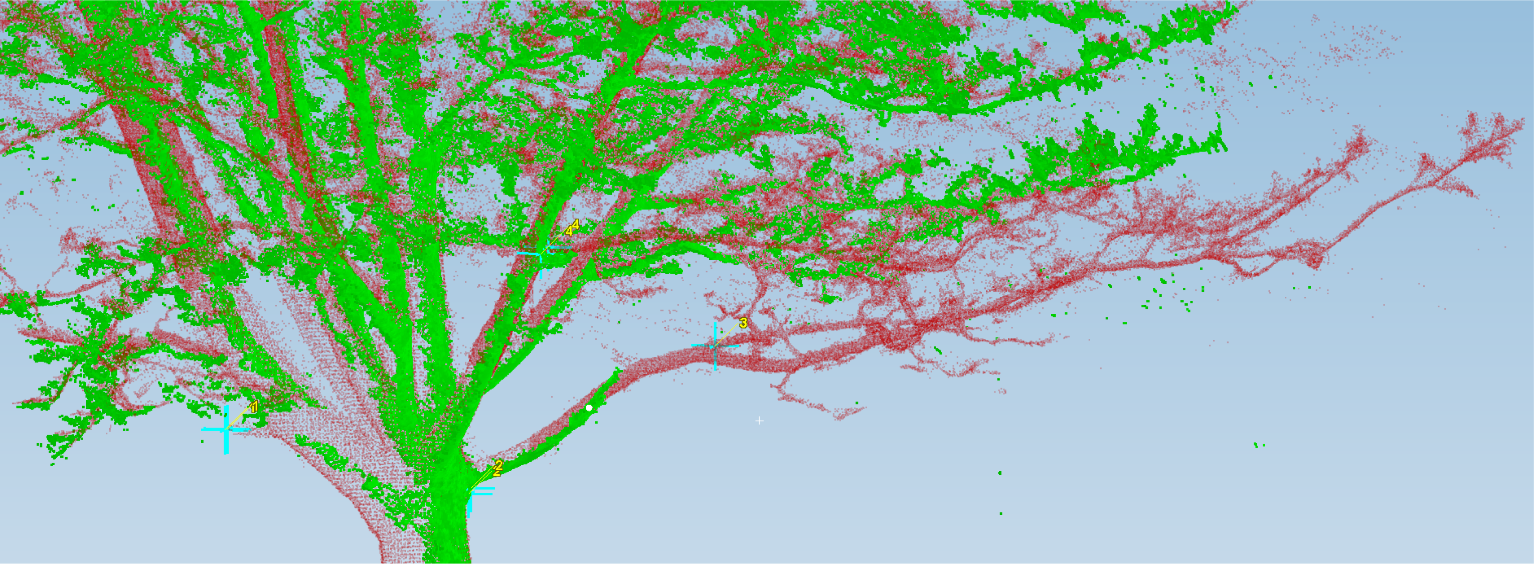
Time series of branch volume and length for the Espoonlahti maple between February 2011 and November 2013 are presented in Table 5. All changes are mean values of 10 modelling runs, with standard deviations of length and volume. The branch length increases in all scans, so the tree growth is visible as an overall trend during the whole period. The volumes increase from scan to scan, except for the April 2012 scan. One reason for this is most likely the loss of two large branches between November 2012 and April 2013 measurements. To estimate the effect of branch loss on the total volume, the results of the QSM for one of the missing branches (total length of 31.4 m and total volume of 18.8 L) (the branch is visible in Figure 9) can be compared to the decrease in branch parameters. The loss of two branches of similar size corresponds well to the decrease of 57 L in branch volume between these two scans. It must be noted, however, that there is a similar change in the stem volume as well, resulting in a total loss of volume of about 115 L. This is about 10% of the total volume of the entire tree.
The variation in the stem volume is partially caused by similar systematic errors and noise as in the case of the aspen branch. Some of it may result from errors in the segmentation, especially in the upper parts, where it is more difficult for the model to choose which one is segmented as the main branch.
3.4. Discussion
To our knowledge, there are no measurements (time series) of tree changes combining this level of efficiency and accuracy. To assess whether the results are realistic, we compared the magnitude of the average branch volume to that measured in laboratory. The branch volume of the Espoonlahti maple was approximately 1000 L and the volume of first and second order branches (i.e., those attached to the stem or the first order branches, respectively) was about 350–430 L in different modelling runs. This is about 2.3–2.8 L per branch, which is the in the order of the total volume (about 1.3 L) of the aspen branch measured in the laboratory. As the reference change of volume for the aspen branch was well reproduced in the measurements, we assume the volume approximation to be realistic.
The major sources of uncertainty were the noise and inaccuracy in measurements, which also affected the modelling. The major error sources can be classified as follows:
- Systematic errors in measurements, caused by, e.g., the size of the laser spot (3.3 mm at about 1.5 m distance, affecting mostly the small branches), tree parts being shadowed by each other, uncertainty in the co-registration of point clouds (where, e.g., wind effects play a role) or noise. The noise points (extra points around the branches) tend to get included in the model, causing overestimation of branch volume.
- Systematic errors in modelling, e.g., the shape approximation error due to the geometric primitives used. Here, we used circular cylinders due to their robustness, but, e.g., cones or elliptic cylinders could be used as well. This aspect is addressed in a forthcoming paper.
- Identifiability errors: changes in the tree shape over time, e.g., the branches bending downwards as they grow, can result in difficulties in identifying the same branches in scans made at different times.
In spite of these errors, the overall accuracy was mostly about ±10%, which is in the order of the laboratory measurements (cf. Section 3.2). In manual measurements, a representative sample of a tree or stand is usually taken. The idea in our approach is to cover all trees/branches in the sample, so achieving 10% accuracy is a promising result. The aspen branch was relatively small (1.3 L) compared to the total volumes of large trees, and hence the errors for small branches are likely to be exaggerated in this case.
The density of points in the point cloud is important when there are not enough points for meaningful segmentation and cylinder fitting. A low density compared to the size of the branches to be reconstructed is problematic for a proper volume estimate with cylinders. Also, some short and thin branches may be left out of the reconstruction, which shows in the total reconstructed branch length. In our samples, the density was high enough, except perhaps for the smallest twigs in the aspen branch. The effect of the registration errors on the maple is probably quite small, but for the aspen branch the effect on the volume can be more significant because of the small size of the branch compared to the registration errors. In the case of input parameters, the size of the surface patches is the most important in reconstruction. Too large patches make the segmentation “rough”; i.e., the separation of the branches does not follow the “true” boundaries which can make the volume too large, but the length is less affected. In our reconstructions, we used 0.5–1.0 mm size patches for the aspen, and 15–30 mm for the maple. We consider these values quite small compared to the size of details in these samples. Smaller patches, if the point density allows, can give more accurate absolute reconstructed values. However, the change detection; i.e., the change in volume and length, is probably not as sensitive to the patch size as the absolute values are, and smaller patches can be expected to better reconstruct the smallest branches which do not contribute much to the volume.
The time consumption of the process (TLS + modelling) per tree varies between 20 and 30 min, depending on the tree size and point density. Our future objective is to develop a version that produces models of all trees in a test plot (consisting of, e.g., 10–20 large trees) from just a few scans. The possible uses of this approach are related to the monitoring of tree growth and mortality and litter production. In this way, there is potential for retrieving the biomass distribution for a set of trees and using this information as ground truth for upscaling tree biomass models into large areas.
Another future issue is to improve the model to account for leaves. The trees presented in this paper have been scanned without leaves, but we are currently developing both measurements and modelling of the leaves, first to reduce their effect on branch models, and, eventually, to include leaf biomass in the analysis.
4. Conclusions
The significant outcome of the study is that our approach based on TLS and QSM is capable of reproducing the trends in the changes in both laboratory and field cases, and the large changes, such as the loss of major branches, could be detected quantitatively from the volumes and observed qualitatively from the consecutive point clouds. Given that the manual measurement of changes in tree structure and dimensions has thus far been carried out by destructive methods, our approach provides for the first time a fast and non-destructive means to monitor the changes in tree structure over time (such as growth and litter production). Since large-scale quantitative information at this level of accuracy has thus far been mostly non-existent, the 10% accuracy achieved by our approach provides a new and unique tool for monitoring tree biomass, canopy structure, litter production, and other important changes.
We are currently working on improving both the measurement and the model accuracy by means of extensive measurement campaigns and model development. An important future objective is to improve the data acquisition with instruments producing less noise, e.g., by the use of pulsed (cf. [12]) or full waveform scanners [33,34], to develop applications for improved monitoring of the growing season and litter production, and to produce large-area (e.g., plot-level) statistics on branching structures (cf. [25]).
Acknowledgments
The authors want to thank Markus Holopainen and Mikko Vastaranta (University of Helsinki) and Antero Kukko (FGI) for co-operation and ideas for the measurements. This study was funded by the Academy of Finland research projects “New techniques in active remote sensing: hyperspectral laser in environmental change detection”, “Mobile hyperspectral laser remote sensing”, “Inverse problems of regular and stochastic surfaces”, “CoE in inverse problems”, and “CoE in Laser Scanning Research”.
Author Contributions
Sanna Kaasalainen, Anssi Krooks, Harri Kaartinen, and Kati Anttila contributed to the TLS and reference measurements. Pasi Raumonen, Anssi Krooks, and Mikko Kaasalainen contributed to the QSM. The analysis of results and writing the article has been carried out by Sanna Kaasalainen, Jari Liski, Pasi Raumonen, and Anssi Krooks. Eetu Puttonen contributed to the TIN models. Raisa Mäkipää contributed to the introduction, discussion, and the laboratory sample.
Conflicts of Interest
The authors declare no conflict of interest.
References
- Intergovernmental Panel on Climate Change (IPCC). Good Practice Guidance for Land Use, Land-Use Change and Forestry, Available online: http://www.ipcc-nggip.iges.or.jp/public/gpglulucf/gpglulucf.html (accessed on 22 January 2014).
- Petersson, H.; Holm, S.; Ståhl, G.; Alger, D.; Fridman, J.; Lehtonen, A.; Lundström, A.; Mäkipää, R. Individual tree biomass equations or biomass expansion factors for assessment of carbon stock changes in living biomass—A comparative study. For. Ecol. Manag 2012, 270, 78–84. [Google Scholar]
- Marklund, L.G. Biomassafunktioner för Tall, Gran Och Björk i Sverige: Biomass Functions for Pine, Spruce and Birch in Sweden; Rapport 45; Sveriges Lantbruksuniversitet: Umeå, Sweden, 1988; p. 73. [Google Scholar]
- Repola, J. Biomass equations for Scots pine and Norway spruce in Finland. Silva Fennica 2009, 43, 625–647. [Google Scholar]
- Pitman, R.; Bastrup-Birk, A.; Breda, N.; Rautio, P. Sampling and Analysis of Litterfall. Part XIII. Manual on Methods and Criteria for Harmonized Sampling, Assessment, Monitoring and Analysis of the Effects of Air Pollution on Forests; UNECE ICP Forests Programme Co-Ordinating Centre: Hamburg, Germany, 2010; p. 16. Available online: http://www.icp-forests.org/Manual.htm (accessed on 22 January 2014). [Google Scholar]
- Liski, J.; Lehtonen, A.; Palosuo, T.; Peltoniemi, M.; Eggers, T.; Muukkonen, P.; Mäkipää, R. Carbon accumulation in Finland’s forests 1922–2004—An estimate obtained by combination of forest inventory data with modelling of biomass, litter and soil. Ann. For. Sci 2006, 63, 687–697. [Google Scholar]
- Harmon, M.; Franklin, J.F.; Swanson, F.J.; Sollins, P.; Gregory, S.V.; Lattin, J.D.; Anderson, N.H.; Cline, S.P.; Aumen, N.G.; Sedell, J.R.; et al. Ecology of coarse woody debris in temperate ecosystems. Adv. Ecol. Res 1986, 15, 133–302. [Google Scholar]
- Tuomi, M.; Laiho, R.; Repo, A.; Liski, J. Wood decomposition model for boreal forests. Ecol. Model 2011, 222, 709–718. [Google Scholar]
- Duursma, R.A.; Mäkelä, A. Summary models for light interception and light-use efficiency of non-homogeneous canopies. Tree Physiol 2007, 27, 859–870. [Google Scholar]
- Medlyn, B.E. Physiological basis of the light use efficiency model. Tree Physiol 1998, 18, 167–176. [Google Scholar]
- Ruimy, A.; Kergoat, L.; Bondeau, A. Comparing global models of terrestrial net primary productivity (NPP): Analysis of differences in light absorption and light-use efficiency. Glob. Chang. Biol 1999, 5, 56–64. [Google Scholar]
- Pueschel, P. The influence of scanner parameters on the extraction of tree metrics from FARO Photon 120 terrestrial laser scans. ISPRS J. Photogramm. Remote Sens 2013, 78, 58–68. [Google Scholar]
- Kankare, V.; Holopainen, M.; Vastaranta, M.; Puttonen, E.; Yu, X.; Hyyppä, J.; Vaaja, M.; Hyyppä, H.; Alho, P. Individual tree biomass estimation using terrestrial laser scanning. ISPRS J. Photogramm. Remote Sens 2013, 75, 64–75. [Google Scholar]
- Pfeifer, N.; Gorte, B.; Winterhalder, D. Automatic reconstruction of single trees from terrestrial laser scanner data. Int. Arch. Photogramm. Remote Sens. Spat. Inf. Sci 2004, 35, 114–119. [Google Scholar]
- Kaasalainen, S.; Hyyppä, J.; Karjalainen, M.; Krooks, A.; Lyytikäinen-Saarenmaa, P.; Holopainen, M.; Jaakkola, A. Comparison of terrestrial laser scanner and synthetic aperture radar data in the study of forest defoliation. Int. Arch. Photogramm. Remote Sens. Spat. Inf. Sci 2010, 38, 82–87. [Google Scholar]
- Hunter, M.O.; Keller, M.; Victoria, D.; Morton, D.C. Tree height and tropical forest biomass estimation. Biogeosciences 2013, 10, 8385–8399. [Google Scholar]
- Liang, X.; Hyyppä, J.; Kaartinen, H.; Holopainen, M.; Melkas, T. Detecting changes in forest structure over time with bi-temporal terrestrial laser scanning data. ISPRS Int. J. Geo-Inf 2012, 1, 242–255. [Google Scholar]
- Holopainen, M.; Vastaranta, M.; Kankare, M.; Räty, M; Vaaja, M.; Liang, X.; Yu, X.; Hyyppä, J.; Hyyppä, H.; Viitala, R.; et al. Biomass estimation of individual trees using stem and crown diameter TLS measurements. Int. Arch. Photogramm. Remote Sens. Spat. Inf. Sci 2011, 38, 91–95. [Google Scholar]
- Côté, J.-F.; Widlowski, J.-L.; Fournier, R.A.; Verstraete, M.M. The structural and radiative consistency of three-dimensional tree reconstructions from terrestrial LiDAR. Remote Sens. Environ 2009, 113, 1067–1081. [Google Scholar]
- Dassot, M.; Colin, A.; Santenoise, P.; Fournier, M.; Constant, T. Terrestrial laser scanning for measuring the solid wood volume, including branches, of adult standing trees in the forest environment. Comput. Electron. Agric 2012, 89, 86–93. [Google Scholar]
- Keightley, K.E.; Bawden, G.W. 3D volumetric modeling of grapevine biomass using Tripod LiDAR. Comput. Electron. Agric 2010, 74, 305–312. [Google Scholar]
- Danjon, F.; Reubens, B. Assessing and analyzing 3D architecture of woody root systems, a review of methods and applications in tree and soil stability, resource acquisition and allocation. Plant Soil 2008, 303, 1–34. [Google Scholar]
- Liski, J.; Kaasalainen, S.; Raumonen, P.; Akujärvi, A.; Krooks, A.; Repo, A.; Kaasalainen, M. Indirect emissions of forest bioenergy: Detailed modeling of stump-root systems. GCB Bioenergy 2014. in press. Available online: http://onlinelibrary.wiley.com/doi/10.1111/gcbb.12091/abstract (accessed on 27 January 2014). [Google Scholar]
- Godin, C.; Costes, E.; Sinoquet, H. A method for describing plant architecture which integrates topology and geometry. Ann. Bot 1999, 84, 343–357. [Google Scholar]
- Raumonen, P.; Kaasalainen, M.; Åkerblom, M.; Kaasalainen, S.; Kaartinen, H.; Vastaranta, M.; Holopainen, M.; Disney, M.; Lewis, P. Fast automatic precision tree models from terrestrial laser scanner data. Remote Sens 2013, 5, 491–520. [Google Scholar]
- Hosoi, F.; Nakai, Y.; Omasa, K. 3-D voxel-based solid modeling of a broad-leaved tree for accurate volume estimation using portable scanning LiDAR. ISPRS J. Photogramm. Remote Sens 2013, 82, 41–48. [Google Scholar]
- Bucksch, A.; Lindenbergh, R. CAMPINO—A skeletonization method for point cloud processing. ISPRS J. Photogramm. Remote Sens 2008, 63, 115–127. [Google Scholar]
- Vonderach, C.; Voegtle, T.; Adler, P. Voxel-based approach for estimating urban tree volume from terrestrial laser scanning data. Int. Arch. Photogramm. Remote Sens. Spat. Inf. Sci 2012, 39, 451–456. [Google Scholar]
- Olsoy, P.J.; Glenn, N.F.; Clark, P.E.; Derryberry, D.R. Aboveground total and green biomass of dryland shrub derived from terrestrial laser scanning. ISPRS J. Photogramm. Remote Sens 2014, 88, 166–173. [Google Scholar]
- Axelsson, P. DEM generation from laser scanner data using adaptive TIN models. Int. Arch. Photogramm. Remote Sens. Spat. Inf. Sci 2000, 33, 110–117. [Google Scholar]
- Sithole, G.; Vosselman, G. Experimental comparison of filter algorithms for bare-Earth extraction from airborne laser scanning point clouds. ISPRS J. Photogramm. Remote Sens 2004, 59, 85–101. [Google Scholar]
- Cao, J.; Tagliasacchi, A.; Olson, M.; Zhang, H.; Su, Z. Point Cloud Skeletons via Laplacian-Based Contraction. Proceedings of 2010 IEEE Conference on Shape Modeling International, Aix-en-Provence, France, 21–23 June 2010; pp. 187–197.
- Yang, X.; Strahler, A.H.; Schaaf, C.B.; Jupp, D.L.B.; Yao, T.; Zhao, F.; Wang, Z.; Culvenor, D.S.; Newnham, G.J.; Lovell, J.L.; et al. Three-dimensional forest reconstruction and structural parameter retrievals using a terrestrial full-waveform lidar instrument (Echidna®). Remote Sens. Environ 2013, 135, 36–51. [Google Scholar]
- Van Leeuwen, M.; Coops, N.C.; Hilker, T.; Wulder, M.A.; Newnham, G.J.; Culvenor, D.S. Automated reconstruction of tree and canopy structure for modeling the internal canopy radiation regime. Remote Sens. Environ 2013, 136, 286–300. [Google Scholar]


| Scanner | Leica HDS6100 |
|---|---|
| Wavelength | 650–690 nm |
| Field of view | 360° × 310° |
| Point separation | 0.036° |
| Beam diameter | 3 mm |
| Beam divergence | 0.22 mrad |
| Maximum Range | 79 m |
| Measurement | Laboratory (aspen) | Espoonlahti (maple) |
|---|---|---|
| Number of points | 390,000–460,000 | 1–5 million |
| Horizontal distance between scanner and branch/tree stem | 1.5–1.9 m | 7–12 m |
| Average point density | 11–25 points /cm2 | 2–5 points/cm2 |
| Cut 1 (L) | Cut 2 (L) | Cut 3A (L) | Cut 3B (L) | |
|---|---|---|---|---|
| Reference | −0.06 | −0.06 | −0.08 | −0.08 |
| QSM | −0.02 | −0.06 | −0.11 | −0.11 |
| Reference, cumulative | −0.06 | −0.11 | −0.19 | −0.19 |
| QSM, cumul. | −0.02 | −0.08 | −0.18 | −0.18 |
| Cut 1 (m) | Cut 2 (m) | Cut 3A (m) | Cut 3B (m) | |
|---|---|---|---|---|
| Reference | −3.85 | −7.25 | −10.43 | −10.43 |
| Reference (>5 cm) | −3.08 | −5.37 | −7.97 | −7.97 |
| QSM | −2.29 | −5.06 | −6.53 | −6.37 |
| Tree Parameters | February 2011 | November 2011 | November 2012 | April 2013 | November 2013 |
|---|---|---|---|---|---|
| Branch vol. (L) | 865 ± 96 | 922 ± 106 | 1107 ± 82 | 1050 ± 87 | 1298 ± 98 |
| Stem vol. (L) | 165 ± 42(*) | 402 ± 43 | 438 ± 32 | 379 ± 133 | 452 ± 40 |
| Total vol. (L) | 1013 ± 97(*) | 1324 ± 92 | 1545 ± 57 | 1429 ± 105 | 1750 ± 101 |
| Branch len. (m) | 1270 ± 114 | 1282 ± 88 | 1590 ± 67 | 1733 ± 116 | 1895 ± 119 |
(*)Part of the stem was covered by snow in February 2011.
© 2014 by the authors; licensee MDPI, Basel, Switzerland This article is an open access article distributed under the terms and conditions of the Creative Commons Attribution license (http://creativecommons.org/licenses/by/3.0/).
Share and Cite
Kaasalainen, S.; Krooks, A.; Liski, J.; Raumonen, P.; Kaartinen, H.; Kaasalainen, M.; Puttonen, E.; Anttila, K.; Mäkipää, R. Change Detection of Tree Biomass with Terrestrial Laser Scanning and Quantitative Structure Modelling. Remote Sens. 2014, 6, 3906-3922. https://doi.org/10.3390/rs6053906
Kaasalainen S, Krooks A, Liski J, Raumonen P, Kaartinen H, Kaasalainen M, Puttonen E, Anttila K, Mäkipää R. Change Detection of Tree Biomass with Terrestrial Laser Scanning and Quantitative Structure Modelling. Remote Sensing. 2014; 6(5):3906-3922. https://doi.org/10.3390/rs6053906
Chicago/Turabian StyleKaasalainen, Sanna, Anssi Krooks, Jari Liski, Pasi Raumonen, Harri Kaartinen, Mikko Kaasalainen, Eetu Puttonen, Kati Anttila, and Raisa Mäkipää. 2014. "Change Detection of Tree Biomass with Terrestrial Laser Scanning and Quantitative Structure Modelling" Remote Sensing 6, no. 5: 3906-3922. https://doi.org/10.3390/rs6053906