Article

Comparing Two Photo-Reconstruction Methods to Produce High Density Point Clouds and DEMs in the Corral del Veleta Rock Glacier (Sierra Nevada, Spain)

by
Álvaro Gómez-Gutiérrez
1,*,
José Juan De Sanjosé-Blasco
2,
Javier De Matías-Bejarano
2 and
Fernando Berenguer-Sempere
2
1
GeoEnvironmental Research Group, University of Extremadura, Avda. De la Universidad s/n, 10071 Cáceres, Spain
2
Geomatics Engineering Research Group, University of Extremadura, Avda. De la Universidad s/n, 10071 Cáceres, Spain
*
Author to whom correspondence should be addressed.
Remote Sens. 2014, 6(6), 5407-5427; https://doi.org/10.3390/rs6065407
Submission received: 28 February 2014 / Revised: 30 May 2014 / Accepted: 3 June 2014 / Published: 11 June 2014
(This article belongs to the Special Issue Remote Sensing in Geomorphology)

Abstract

:
In this paper, two methods based on computer vision are presented in order to produce dense point clouds and high resolution DEMs (digital elevation models) of the Corral del Veleta rock glacier in Sierra Nevada (Spain). The first one is a semi-automatic 3D photo-reconstruction method (SA-3D-PR) based on the Scale-Invariant Feature Transform algorithm and the epipolar geometry theory that uses oblique photographs and camera calibration parameters as input. The second method is fully automatic (FA-3D-PR) and is based on the recently released software 123D-Catch that uses the Structure from Motion and MultiView Stereo algorithms and needs as input oblique photographs and some measurements in order to scale and geo-reference the resulting model. The accuracy of the models was tested using as benchmark a 3D model registered by means of a Terrestrial Laser Scanner (TLS). The results indicate that both methods can be applied to micro-scale study of rock glacier morphologies and processes with average distances to the TLS point cloud of 0.28 m and 0.21 m, for the SA-3D-PR and the FA-3D-PR methods, respectively. The performance of the models was also tested by means of the dimensionless relative precision ratio parameter resulting in figures of 1:1071 and 1:1429 for the SA-3D-PR and the FA-3D-PR methods, respectively. Finally, Digital Elevation Models (DEMs) of the study area were produced and compared with the TLS-derived DEM. The results showed average absolute differences with the TLS-derived DEM of 0.52 m and 0.51 m for the SA-3D-PR and the FA-3D-PR methods, respectively.

1. Introduction

The monitoring and assessment of glacier dynamic-retreat provides basic information for future and current research on the impact of climate change at global and regional scales. Among glaciers, rock glaciers present a special interest because they are considered as key indicators of environmental change in mountainous regions. A rock glacier creeps downslope by force of gravity and is composed of angular rock debris and subsurface ice, exhibiting lobate or tongue-shaped forms [1].
The first known trial to monitor and quantify the movement of a rock glacier dates from 1948 in Clear Creek [2]. Since then, technical advances and innovations have been significant to improving our knowledge: geomatics techniques, geophysical methods, dating techniques, etc.
In the specific case of geomatics, there are numerous techniques for monitoring and quantifying the dynamic and morphology of glaciers such as the measurement of fixed points (rods or pins), total stations (e.g., [3]), GPS (e.g., [4]), LIDAR (e.g., [5]), Terrestrial Laser Scanners (TLS; e.g., [6]), aerial photogrammetry (e.g., [7]), satellite images (e.g., [8]) and terrestrial photogrammetry or photo-reconstruction methods (e.g., [9]). The monitoring in mountainous areas with low accessibility, steep slopes and ice or snow during long periods of the year is usually difficult and costly. In 2001, Baltsavias et al. [5] described the measurement density and/or accuracy of glacier monitoring techniques as insufficient. During the last decade, a great advance has been experienced in the field of monitoring methods with more accurate, cheaper, lighter and simpler equipment (e.g., TLS or GPS). A comprehensive and detailed description of the techniques used for topographic, spatial and thematic mapping of glaciers in addition to a large set of references can be found in [10].
Rock glaciers and debris-covered glaciers are still poorly understood and represent a very interesting and active field of present research [11,12]. In the specific case of rock glacier monitoring, one of the main limitations is that mean annual creep velocities are typically in the range of centimeters to decimeters (sometimes meters) whilst surface lowering due to permafrost degradation has been reported to be in the centimeter range [1]. These low creep velocities require the application of accurate high resolution techniques such as aerial photogrammetry [7]. There are dozens of examples in the literature about the use of aerial photogrammetry to monitor changes in rock glaciers or alpine permafrost surfaces, e.g., [7,1316]. The recent development of Unmanned Aerial Systems or Unmanned Aerial Vehicles (UAS or UAV) has resulted in a significant reduction in cost for aerial surveys and photogrammetry projects. However, their use for monitoring glaciers (and specifically rock glaciers) is not widespread (a recent exception is [17]). In general, aerial images acquired using conventional airborne methods are well suited to derive DEMs or orthophotographs, but they present limitations for motion detection in small glaciers. On the other hand, UAVs allow the acquisition of high resolution images due to its possible low flight altitude [18].
Terrestrial photogrammetry has also been widely used for mapping or monitoring rock glaciers (e.g., [1921]). However, drawbacks of terrestrial photogrammetry against aerial photogrammetry have been highlighted in the literature [19], mainly, area-wide mapping difficulties and heterogeneous horizontal accuracy. On the other hand, sensing from vertical (or nearly vertical) viewing angles means that steep slopes are registered with strong restrictions [22]. The classical geodetic survey provides accurate measurements for estimating rock glacier superficial flow velocities. The most common classical instruments used to carry out classical geodetic surveys in rock glaciers and debris-covered glaciers are total stations [3,23,24] and GPS or DGPS [23,2528]. These techniques ensure centimeter-level accuracies; however, GPS-DGPS cannot be used in certain cirques, where the walls are close to the measured points because the satellite signal is often interrupted or rebounds of the multipath signal are experienced and the resulting accuracy is too low [23]. Recently, De Sanjosé et al. [23] analyzed a variety of geomatic techniques available for monitoring rock glaciers and ice patches in Spain: total station, GPS, close-range classical photogrammetry and TLS. This research covered a time span of 20 years and the authors concluded that there is no optimal technique for monitoring rock glaciers; depending on their characteristics, morphology and structure, different geomatic instruments and techniques can be applied.
In the last years, laser-based technologies have been applied with the aim of quantifying the displacement and dynamic of rock glaciers from terrestrial devices (i.e., Terrestrial Laser Scanner: TLS, e.g., [22,23,2931]) or aerial platforms (Airborne Laser Scanning: ALS, e.g., [3235]). The use of these modern instruments produced more accurate and denser datasets with less logistical efforts and time, leading to lower costs and greater quality of field surveys [22].
Also recently, photogrammetry (aerial and terrestrial) has experienced a revival due to several facts, but mainly due to the innovations experienced in the field of computer vision. Recent developments made in three-dimensional photo-reconstruction techniques (3D-PR), such as the simultaneous use of Structure from Motion (SfM; [36]) and MultiView-Stereo (MVS; [37]), have allowed for the attainment of high resolution 3D point clouds and meshes [3840]. These cartographical products (3D point clouds and meshes) are achieved using only oblique images from consumer non-calibrated and non-metric cameras as input. It is likely that, within the next decade, these 3D-PR methods will be widely used in the geosciences, mainly in geomorphology and geomorphometry. Until now, the few studies using photo-reconstruction techniques in these disciplines have concluded that more work needs to be done in order to analyze their performance over a wider range of landforms, processes, scales and environments [4144].
Therefore, the objectives of this paper are:
(1)
to produce dense point clouds and high resolution Digital Elevation Models (DEMs) for the Corral del Veleta rock glacier (Sierra Nevada, Spain) by means of two free 3D-PR procedures (a self-implemented stereo feature-based semi-automatic method and a fully automatic method based on the software 123D Catch that uses SfM and MVS algorithms);
(2)
to compare and analyze the quality of the point clouds and the DEMs obtained by means of the two 3D-PR methods as compared with a point cloud and a DEM obtained by means of a Terrestrial Laser Scanner (TLS); and
(3)
to evaluate the usefulness of these methods to register changes in the glacier dynamic.

2. Study Area

The Corral del Veleta rock glacier (Figure 1: 37°3′N–3°21′W) is located in Sierra Nevada (Spain), in a depression known as the Corral del Veleta (Figure 1c,d) which is a north face-oriented cirque at the bottom of the Veleta peak (3398 masl). The existence of fossil ice and permafrost under the detritic cover in the Corral del Veleta was discovered in 1998 using geophysical prospection and direct sampling [45]. After this discovery, the Corral del Veleta rock glacier was identified as the southernmost rock glacier in Europe with a latitude of 37°3′ [46]. Due to this special location, monitoring and assessment of the Corral del Veleta rock glacier dynamic presents a great scientific interest because it is assumed as a key indicator on the effects of climate change in the region. The progressive retreat of the historical glacier of the Corral del Veleta rock glacier towards the end of the Little Ice Age led to the transformation from a “white” glacier to the “black” or rock glacier, mainly due to the continuous supply of boulders originating from the incessant destruction of the wall which incrementally covered the ice [45,47]. The main characteristics of the Corral del Veleta rock glacier are presented in Table 1.
Since 2001, an intensive study of the Corral del Veleta rock glacier has been carried out using several geomatic techniques (total station, photogrammetry and GPS, [9]). These works have shown that relict ice and permafrost of the glacier are in a continuous process of deglaciation due to subsidences in the clastic layer and the decrease in the link between subsurface frozen bodies.

3. Methodology

In this work, two methods based on computer vision are used and compared to produce high resolution point clouds and DEMs of the Corral del Veleta rock glacier. The first one is a Semi-Automatic 3D-PR method (hereafter called SA) based on the use of Scale-Invariant Feature Transform algorithm (SIFT, [48]) and epipolar geometry that needs as input oblique photographs and camera calibration parameters and produces as a result 3D point clouds. The second method is fully automatic (hereafter called FA) and is based on the recently released free software 123D Catch that uses the SfM and the MVS algorithms together and only needs as input oblique photographs and some measurements in order to scale and geo-reference the resulting 3D point cloud-model (i.e., the camera certificate and the parameters are not necessary). 123D Catch software was used because it is free and extremely simple to use, it represents an all-to-one solution and, to the best of our knowledge, its suitability has as of yet been rarely tested for applications in the geosciences [44]. To the best of our knowledge, this is the first experiment using 123D Catch software to produce dense point clouds and high resolution DEMs in a rock glacier. These environments represent a special challenge for SfM-based methods because of their complexity and variability. The six images used in the photo-reconstruction process were acquired with a Canon EOS 5D (which is a SLR consumer-grade device) camera with a fixed-focal distance of 100 mm and an exposure time of 1/160 s (Figure 2). The former parameters were defined after several tests to optimize the visual quality of the images. The six images were selected over the others because of their contrast, geometry and light conditions. These images presented dimensions of 4368 × 2912 pixels and sizes from 10.5 MB to 11.2 MB. The photographs were captured from the top of Veleta peak towards the Corral del Veleta glacier and with the camera parallel to the wall of the Veleta peak at an approximate distance of 300 m (Figure 1c,d). In the case of the Corral del Veleta rock glacier, the distance from the object of interest (the glacier) to the camera is imposed by the topography (Figure 1c,d).
Additionally, a benchmark 3D model was obtained by means of a TLS (Leica C10 Scanstation device) in order to test the quality of the SA and the FA methods. A positional error less than ±6 mm for every 50 m is expected for measurements made with this equipment. Four stations were located around the shape of the glacier and later, point clouds obtained from every station were registered in a unique point cloud using Cyclone software (Leica Geosystem; [49]). The errors calculated during the registration process were always below 0.003 m. Finally, the unique point cloud was transformed to an absolute reference system using 20 control points placed on stable zones (e.g., lateral moraine; Figure 1d) and measured with a GPS in RTK static mode. These control points were established and measured for the previous work by de Matías et al. [9]. The transformation between the absolute coordinate system (defined by the GPS measurements) and the relative (TLS) consisted on a classical rigid 3D transformation, including 3 translations, 3 rotations and one scale factor. The Root Mean Square Error (RMSE) obtained during the georeferencing of the point cloud was 0.03 m. The differences between the SA and the FA methods and the TLS survey were estimated by calculating nearest neighbor point-to-point 3D distances for every point in the cloud using CloudCompare open source software [50] and Girardeau-Montaut et al. [51] method. Note that the former method, based on a 3D frame, against GIS-based approaches (2.5D) are more reliable for 3D datasets but have been rarely used to test photo-reconstruction techniques [44].

3.1. Stereo-Based SIFT Method

A deep description of this method can be found in the paper by De Matías et al. [9]; hence, only a brief summary is given here. The input requirements for the SA procedure are a set of images of the feature to be modelled taken from different viewpoints and the camera calibration parameters (i.e., focal length, coordinates of the principal point and the radial distortion functions). The first stage of the procedure is to extract feature points from each image using the Difference of Gaussian algorithm (DoG) and to store them in a database using SIFT descriptors. Secondly, it is possible to get a set of matching points based on the distance between SIFT descriptors. After that, matches are refined by a robust matching procedure through the epipolar geometry requirement (i.e., matches that do not hold the epipolar geometry constraint are removed from the database). Finally, camera pose is estimated using the camera calibration parameters and exterior orientation system is solved (rotation and translation of cameras or camera pose). For more details about the absolute orientation and the geodetic control, please see [9]. The final result is a point cloud or a 3D model based on meshes with X, Y and Z coordinates obtained by applying the set of projection camera matrices to the features in the database.

3.2. Fully Automatic 3D-PR Software: 123D Catch

Fully automatic photo-reconstruction procedures have been recently incorporated in several software packages in order to produce point clouds and 3D models. Table 2 ([5257]) shows the existing free software that incorporates 3D-PR techniques, among these, 123D Catch was selected because it is free, quite simple to use and represents an all-to-one solution. Two previous works have tested the suitability of this software to produce high resolution 3D models of geological-geomorphological features [44,58]. In [58], Chandler and Fryer reconstructed an aboriginal cave in Australia and Gómez-Gutiérrez et al. [44] used 123D Catch to elaborate 3D models and to estimate headcut retreat rates in a small permanent gully in Spain. Both studies concluded that the accuracy of the models obtained by means of the software is comparable to the accuracy of models produced using TLS equipment.
The performance of 123D Catch is based on the simultaneous use of SfM [36] and MultiView-Stereo [37] techniques, which allows the obtaining of high resolution 3D point clouds or meshes [38,40] using conventional photographs as input. In 123D Catch software, the camera pose and parameters are solved automatically and without the need of control points with real coordinates during the composition of the model. Similarly to the SA method, the SIFT algorithm is used to identify matching features in different images. These features and their characteristics are stored in a database that is used to estimate camera model parameters in a relative coordinate system with an iterative bundle adjustment [59]. The final step consists of using a few control points to scale and georeference the resulting point cloud. In order to georeference this point cloud, the dataset obtained by means of the TLS (with absolute coordinates) was used as benchmark. Natural control points (i.e., rocks; n = 10) were identified in this 3D model and used during the first stage of the georeferencing process (i.e., manual georeferencing using 4-points congruent sets algorithm [60]). Finally, automatic registration was carried out to refine the matching between the resulting point cloud and the TLS dataset with absolute coordinates. CloudCompare software and the algorithm iterative closest point [61] were used for this purpose. The georeferencing process resulted in a RMSE of 0.18 m.

3.3. Elaboration of DEMs

Digital Terrain Models (DTMs), especially DEMs, are instruments commonly used by geomorphologists to describe land surface and produce geomorphological maps. DEMs are powerful tools to describe changes in highly dynamic landscapes (e.g., channels, glaciers, volcanoes, hillslopes affected by mass movements, etc.). In the Corral del Veleta, previous works by de San José et al. [3] had monitored the dynamic of the glacier using fix control points that were measure with Differential GPS (DGPS) and total stations annually (from 2001 to 2005). The former approach allowed for an estimate of the displacement of the fixed points and therefore for an understanding of the glacier dynamic. However, this approach presented two main inconveniences:
(1)
a dense network of points is needed to represent faithfully the dynamic of the whole glacier and
(2)
points are defined by fixed rods that can be lost with time in this changeable environment.
On the other hand, DEMs present a continuous description of the surface and they enable the estimation of volumetric changes between consecutive field surveys. In this work, the point clouds obtained by the SA, the FA and the TLS methods were used to produce high resolution DEMs. To describe the rock glacier surface morphology and to detect changes (for future surveys), the quality of these products was analyzed. The obvious absence of vegetation or other non-ground surface features in the study area facilitated the elaboration of the DEMs. The derived point clouds were meshed as Triangulated Irregular Networks (TINs) and then converted in raster file format using ArcGIS 10.2 software [62] The DEM obtained by means of the point cloud captured by the TLS was considered as benchmark and differences from this DEM to the other DEMs were calculated and analyzed.

4. Results and Discussion

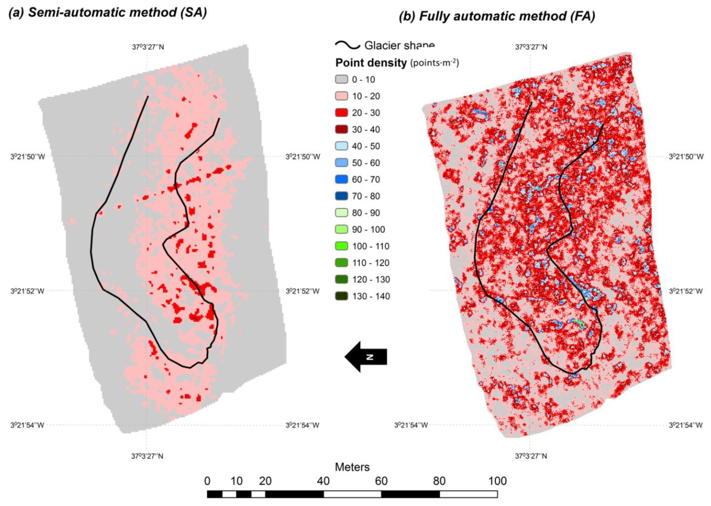
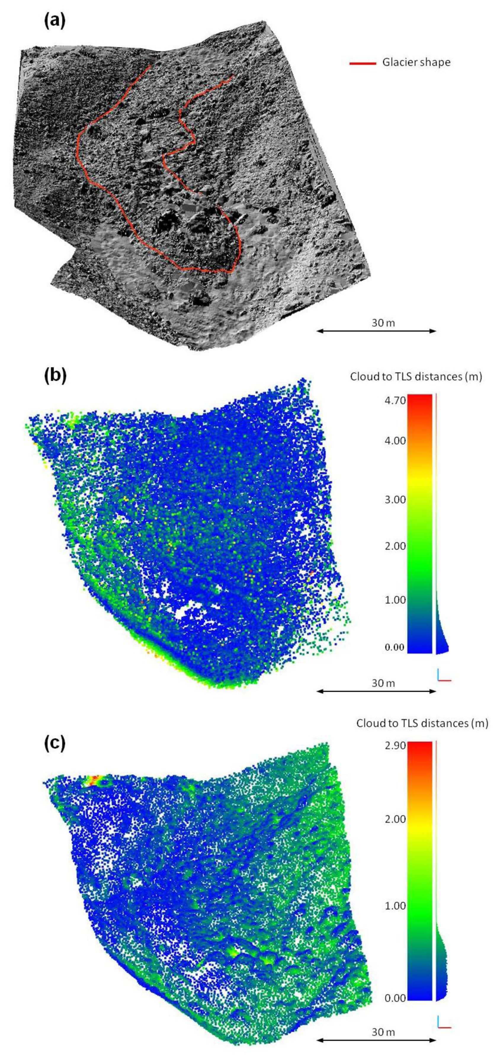
4.1. Point Cloud Characteristics: Accuracy and Density

Dense point clouds were obtained with the two photo-reconstruction methods using as input only six images (Figure 2 and Table 3). However, important differences were observed in the number of points obtained with the SA and FA methods (Table 3). The Autodesk 123D Catch (FA) software produced 2.5 times the number of points obtained by the SA self-implemented procedure. This difference was clearly reflected in the average point spacing (1.6 times higher for the SA method) and average point densities (2.5 times higher for the FA method). According to the figures for the former two parameters (i.e., point spacing and point density) the obtained point clouds are suitable for sub-meter monitoring of the glacier with 8.09 pts·m−2 and 20.58 pts·m−2 for FA and SA respectively. Regarding the spatial distribution of the point densities (Figure 3) for the SA method, the highest densities were found in the central and southern parts of the rock glacier, i.e., in the areas that are present in a central location in all the photographs and nearer to or facing the wall (i.e., the place where the photographs were taken; Figure 1c,d). Point densities decreased from the inner to the outer and northern parts of the study area where the lowest values were experienced, with densities below 10 pts·m−2. In the case of the FA method, the spatial distribution of the point densities is clearly influenced by shadows, sharpness and natural textures of the features in the images (i.e., the rock blocks). In fact, the spatial distribution of large blocks can be deduced from the point density map (Figures 2 and 3b) with high point densities (>30 pts·m−2) registered in lighted faces of the rocks and low densities (<10 pts·m−2) in the shadowed faces. Previous works have described the point density and quality of 3D-PR methods as a function of the density, sharpness and resolution of the photoset in addition to the texture of the features to be modelled [43]. According to the results obtained here and for future surveys, the optimal time of the year (also of the day) to take photographs can be estimated using hillshade digital models that can be calculated easily with a high resolution DEM and any GIS desktop software (e.g., Figure 4a shows a 3D view of a hillshade model calculated with ArcGIS 10.2). In order to produce these hillshade models the location of the sun in the sky is used as input (i.e., azimuth and altitude) and therefore the percentage of the surface illuminated by the sun can be estimated for every hour of every day. There are dozens of online tools free available to estimate the azimuth and the altitude of the sun for a specific day, time and location (e.g., US Naval Observatory [63]). As an alternative, the field work could be planned to be carried out under diffuse illumination (i.e., cloudy conditions) as was proposed by James and Robson [41]. To corroborate this finding, a quantitative simulation is presented in Section 4.2 which is dedicated to the elaboration and analysis of DEMs.
Regarding the accuracies estimated for every point cloud, comparisons with the TLS point cloud showed average distances of 0.28 m and 0.21 m for the SA and the FA methods respectively. These data suggest that in the case of debris rock glacier monitoring sub-meter-level accuracies can be expected using a similar sampling procedure and data processing. The standard deviations and the maximum distances from the clouds to the TLS point cloud are showed in Table 3. According to these accuracies, both methods are suitable for micro-scale and medium-term (from 5 to 10 years intervals) monitoring of the Corral del Veleta rock glacier, taking into account that a recent study has shown that the dynamic of the glacier ranged from 0.05 m to 0.10 m of displacement per year in planimetry and from −0.20 m to −0.25 m per year in altimetry from 2001 to 2005 [3]. In general terms, the suitability of these methods in other rock glaciers should be defined taking into account the creep velocities which are usually in the range of centimeters to decimeters (sometimes meters) whilst surface lowering due to ice melt (i.e., permafrost degradation) has been reported to be in the centimeter range [1]. Figure 4 shows the spatial distribution of cloud-to-cloud distances in a 3D perspective (i.e., nearest neighbor point-to-point distances). The maximum distances were observed in hidden areas for the TLS. As was stated previously, photographs were taken from the top of the mount Veleta towards the Corral del Veleta rock glacier (Figure 1c,d), resulting in an almost-vertical perspective and therefore with no (or only a few) hidden areas. On the other hand, the TLS stations were located in the glacier’s surrounding areas (Figure 1c), resulting in some small hidden areas. For the SA method, 90% of the points in the cloud presented distances to the TLS point cloud less than 0.97 m while for the FA method 90% of the points showed distances to the TLS point cloud less than 0.70 m. Note that the histograms of the distances to the TLS point cloud are included beside the legend in Figure 4b,c.
Recently, some researchers have provided dimensionless estimations of the quality of 3D-PR models by means of the relative precision ratio (i.e., measurement precision/observation distance). James and Robson [41] provided values around 1:1000 whilst Gómez-Gutiérrez et al. [44] estimated values ranging from 1:372 to 1:1167. Here, values of 1:1071 and 1:1429 were calculated for the SA and the FA method respectively. In spite of being different geomorphological features, a hand sample volcanic bomb, a coastal cliff and the summit crater of a volcano in [41] and small gully headcuts in [44], figures obtained here were in the same order of magnitude (≈1:1000). According to these figures, to achieve 1 m of accuracy with the SA method the camera should be located at most at 1071 m, whereas for the FA method photographs could be taken at most from a 358 m distance. Again, these results point to an outperformance of the FA procedure. The distance from camera to the target is a crucial factor for surveying areas with limited accessibility, such as high mountains with steep slopes and ice or snow during long periods of the year. The figures presented here for the relative precision ratio could work as guidance for the analysis of the camera optimal—maximum distances to the object of interest in the frame of photo-reconstruction surveys in high mountain areas. For example, if an accuracy smaller than 1 m is required for a certain survey, distances from the camera to the object closer than approximately 1 km are recommended. Additionally, using GIS software makes it quite simple to implement two rules based on the maximum distance to the feature of interest (with a buffer analysis) and the maximum visibility (with a viewshed analysis) to detect the optimal locations of the camera.

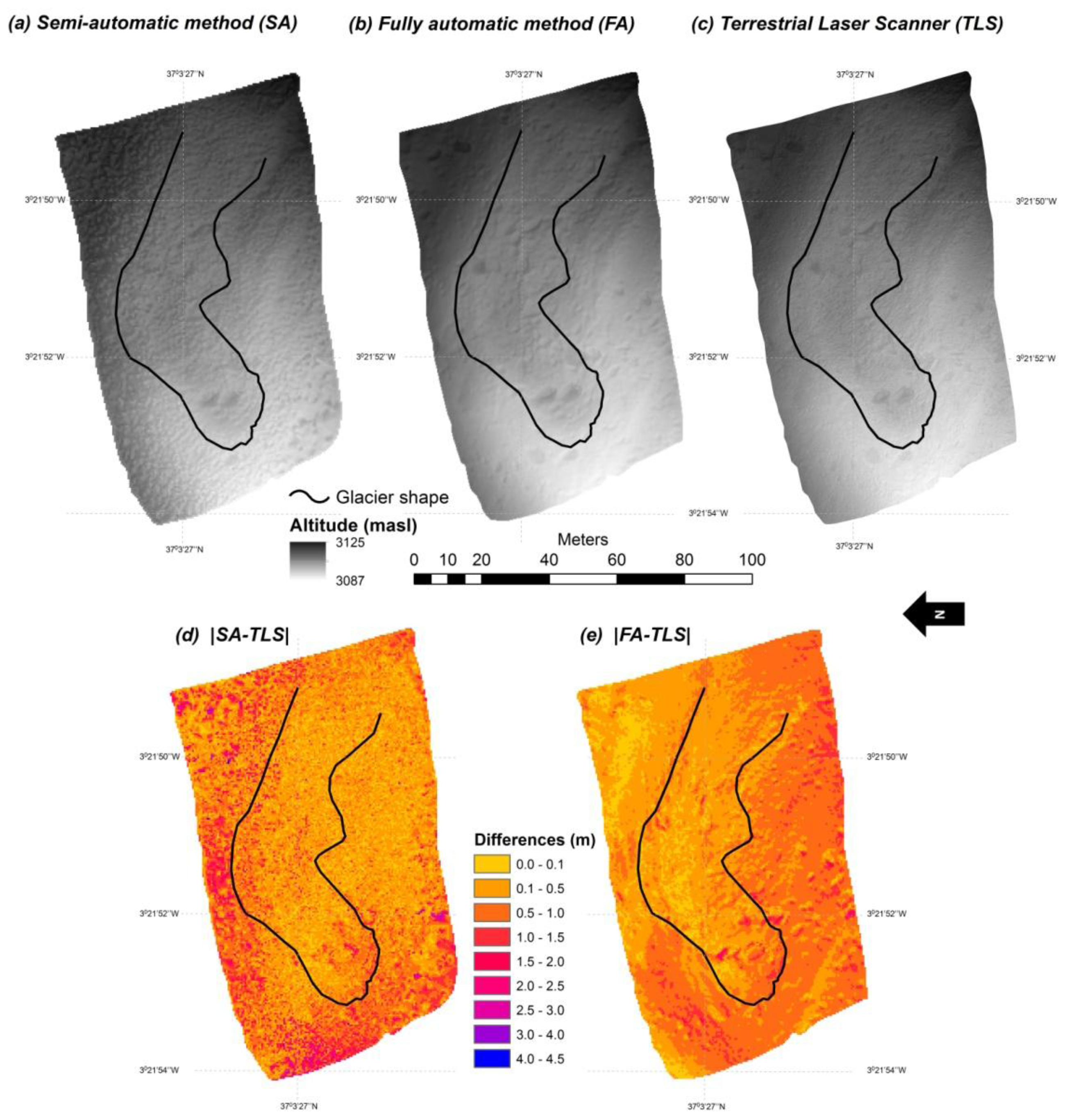
4.2. Digital Elevation Models

According to the point density and the average point spacing, DEMs with pixel sizes of 0.50 m, 0.25 m and 0.05 m were elaborated for the SA method, the FA method and the TLS dataset, respectively. The statistical description of these DEMs is presented in Table 4. These figures highlight that the DEMs obtained by means of the SA and the FA methods are quite similar from a statistical viewpoint and, at the same time, fit properly with the DEM obtained using the TLS point cloud that was defined as benchmark (with the R coefficients always above 0.99). Even the histograms showed a similar profile; however, a quick visual analysis of the DEMs (Figure 5a–c) reveals that the DEM produced using the SA point cloud (Figure 5a) presents a grainy texture which is not present in the DEMs produced with the FA and the TLS methods (Figure 5b,c respectively). This highly local variability of the Z values in the SA DEM is clearly visible in Figure 5d where absolute differences between the SA and the TLS DEMs are presented. In general terms, differences between the SA DEM and the TLS DEM were higher than the differences between the FA DEM and the TLS DEM. Figure 5d,e show a quite similar pattern than the one calculated using the approach by Girardeau-Montaut (Figure 4b,c, [51]) to estimate the nearest neighbor point-to-point 3D distances, with the highest differences in the northwest and in the south for the SA and the FA methods, respectively. Therefore, the method proposed by Girardeau-Montaut [51] to estimate cloud-to-cloud distances for point clouds seems to be a good indicator of the later quality of the DEMs.
As was stated before, the optimal time of the year to take the photographs (even of the day) could be estimated using hillshade digital models (i.e., shaded relief models) that can be calculated with a high resolution DEM (TLS DEM in this case) and any GIS desktop software. To corroborate the relationship between the quality of the DEM obtained (by means of the FA method) and the amount of shadowed-lighted areas in the photographs, a hillshade model was calculated simulating the location of the sun in the sky during the field survey. To do this, the azimuth and altitude of the sun were estimated using the on-line application by the US Naval Observatory website [63]. ArcGIS software was used to produce the shaded relief model that shows the lowest values for shadowed areas, whilst lighted areas present the highest values. Figure 6 shows the obtained shaded relief model and one of the photographs captured during the field work (after being orthorectified). The correspondence between the two images is clear. Finally, areas with different hillshade values were grouped and their absolute errors (i.e., the absolute difference with the TLS DEM) were calculated. As can be deduced from Table 5, the areas with the highest values for the hillshade model (lighted areas) presented the lower absolute errors while shadowed areas experienced the highest absolute errors.
With the purpose of showing the applicability of the proposed methodology, the optimal hour to capture the photographs throughout 28 August 2014, when the next field survey is planned, was calculated. Hillshade digital models were produced for every hour of the day (from 8:00 to 21:00, i.e., when the sun is visible from this location) and the optimal one was assumed as the time for which the average value of the pixels in the shaded relief models reaches the maximum (Figure 7a). The results pointed to 14:00 as the optimal hour to take the photographs on 28 August 2014 in the study area. Figure 7 shows the values of this simulation and the estimated optimal hillshade. Significant differences were observed between Figure 6b (representing the simulated shaded relief during the capture of the photographs for the present work) and Figure 7b (the shaded relief model for the estimated optimal time on 28 August 2014).

4.3. Comparison of Techniques

The SA and the FA methods allow replacing expensive photogrammetric flights with almost-free surveys based on photographs taken from the top of the surrounding mountains. They also allow the elimination of extensive office work by human operators in order to obtain 3D point clouds or contours, replacing classical digital photogrammetric restitution with FA or SA methods. The SA method requires a higher amount of input data (photographs, camera calibration parameters and control points), whereas the FA just need the photographs and a few control points to produce dense geo-referenced point clouds and high resolution DEMs. The advantages of both techniques over other methods such as total stations, traditional aerial photogrammetry or terrestrial photogrammetry, GPS and TLS, have been confirmed in the present study and in the recent literature:
-
They require little expertise because the processing is almost automatic [41], mainly in the case of FA method.
-
The accuracy of 3D-PR methods depends on several factors; one of the most important parameters being the distance from the camera to the target. Some recent works have reported similar figures to the most accurate methods available today (such as TLS or traditional photogrammetry, [41,42,53,64]).
-
Both techniques are cheaper and less time-consuming as compared to other methods/techniques. In the case of the FA procedure, we would like to highlight that the processing is run in the cloud, therefore the company (Autodesk) will have access to your images. The processing time is reduced but your images need to be uploaded to the company’s servers.
Another important point is that both techniques overcome the restrictions associated with vertical (or almost vertical) viewing angles commonly used in aerial photogrammetry or remote sensing when applied to steep slopes. Even these kinds of photo-reconstruction procedures allow the combination of aerial and ground photo-datasets. Finally, a qualitative comparison of the three methods used here was carried out (Table 6) in order to identify the optimal one in terms of capture and processing time, cost of the equipment, expertise requirements and accuracy and quality of the resulting products (i.e., point clouds and DEMs). This analysis is based on our experiences throughout the development of the present research.

5. Conclusions

In this paper, two methodologies based on 3D photo-reconstruction techniques were applied and tested with the aim of producing dense point clouds and high resolution Digital Elevation Models (DEMs) of the Corral del Veleta rock glacier in Sierra Nevada (Spain). The first one is a Semi-Automatic (SA) method based on the use of the Scale-Invariant Feature Transform algorithm and the epipolar geometry. The second methodology is Fully-Automatic (FA) and is based on the free available and recently released Autodesk 123D Catch software. The accuracy of the resulting point clouds was tested using as benchmark a 3D model captured by a Terrestrial Laser Scanner (TLS). Both methods produced point clouds suitable for sub-meter monitoring of the glacier with average distances to the TLS point cloud of 0.28 m and 0.21 m for the SA and the FA methods, respectively. The estimation of the relative precision ratio (i.e., measurement precision/observation distance) resulted in values of 1:1071 (SA) and 1:1429 (FA); showing that to achieve 1 m of accuracy with the FA method, a camera (with similar characteristics to the one used here, i.e., Canon EOS 5D) should be located, at most, to 1429 m from the target.
Moreover, it was found that the global accuracy of the point cloud obtained by the FA method is related to shadows, sharpness and natural textures of the features shown in the images. According to this finding, a methodology to estimate the optimal time-date to take the photographs (for FA 3D photo-reconstruction procedures) was proposed. The method is based on simulating shadows in the study area using a high resolution DEM and the location of the sun in the sky for different moments to produce sequential shaded relief models (i.e., hillshades). The optimal time-date is selected as the one that maximizes the average hillshade value in the shaded relief models.
Finally, DEMs were produced using the point clouds obtained by means of the SA and the FA methods and compared with a DEM elaborated using the TLS point cloud. The results showed average absolute differences with TLS DEM of 0.52 m and 0.51 m for the SA and the FA DEMs, respectively.
Future work should be focused on testing: (i) the performance of different 3D photo-reconstruction methods over other landforms, processes, scales and environments, and (ii) the use of photographs improved-optimized by means of High Dynamic Range (HDR) techniques.

Acknowledgments

This research was funded by the Government of Extremadura region, FEDER (file numbers GR10071 and RNM017) and the Ministry of Economy and Competitiveness (CGL2011-23361).
  • Author ContributionsÁlvaro Gómez-Gutiérrez implemented the research design, performed data analysis and executed the manuscript writing. José Juan de San José-Blasco carried out field work and provided geodesic support in order to georeference the models. Javier de Matías developed the SA method and carried out field work and data processing and analysis. Fernando Berenguer-Sempere carried out field work and TLS data processing and analysis.

Conflicts of Interest

The authors declare no conflict of interest.

References

  1. Kaufmann, V. The evolution of rock glacier monitoring using terrestrial photogrammetry: The example of äusseres hochebenkar rock glacier (Austria). Austrian J. Earth Sci 2012, 105, 63–77. [Google Scholar]
  2. Wahrhaftig, C. Foreword. In Rock Glaciers; Giardino, J.R., Shroder, J.F., Vitek, J.D., Eds.; Allen & Unwin: Boston, MA, USA, 1987; pp. VII–XII. [Google Scholar]
  3. De SanJosé, J.J.; Atkinson, A.D.J.; Salvador, F.; Gómez, A. Application of geomatic techniques to monitoring of the dynamics and to mapping of the veleta rock glacier (Sierra Nevada, Spain). Z. Geomorphol 2007, 51, 79–89. [Google Scholar]
  4. Aoyama, Y.; Doi, K.; Shibuya, K.; Ohta, H.; Tsuwa, I. Near real-time monitoring of flow velocity and direction in the floating ice tongue of the shirase glacier using low-cost GPS buoys. Earth Planets Space 2013, 65, 103–108. [Google Scholar]
  5. Baltsavias, E.P.; Favey, E.; Bauder, A.; Bosch, H.; Pateraki, M. Digital surface modelling by airborne laser scanning and digital photogrammetry for glacier monitoring. Photogramm. Rec 2001, 17, 243–273. [Google Scholar]
  6. Kerr, T.; Owens, I.; Rack, W.; Gardner, R. Using ground-based laser scanning to monitor surface change on the rolleston glacier, New Zealand. J. Hydrol. N. Z 2009, 48, 59–72. [Google Scholar]
  7. Kääb, A.; Haeberli, W.; Gudmundsson, G.H. Analysing the creep of mountain permafrost using high precision aerial photogrammetry: 25 years of monitoring Gruben rock glacier, Swiss Alps. Permafr. Periglac. Process 1997, 8, 409–426. [Google Scholar]
  8. Paul, F.; Kääb, A.; Haeberli, W. Recent glacier changes in the Alps observed by satellite: Consequences for future monitoring strategies. Glob. Planet. Chang 2007, 56, 111–122. [Google Scholar]
  9. De Matías, J.; de Sanjosé, J.; López-Nicolás, G.; Sagüés, C.; Guerrero, J. Photogrammetric methodology for the production of geomorphologic maps: Application to the Veleta rock glacier (Sierra Nevada, Granada, Spain). Remote Sens 2009, 1, 829–841. [Google Scholar]
  10. Pellikka, P.; Rees, W.G. Remote Sensing of Glaciers. Techniques for Topographic, Spatial and Thematic Mapping of Glaciers; Taylor & Francis Group: London, UK, 2010. [Google Scholar]
  11. Mayer, C.; Lambrecht, A.; Belò, M.; Smiraglia, C.; Diolaiuti, G. Glaciological characteristics of the ablation zone of Baltoro Glacier, Karakoram, Pakistan. Ann. Glaciol 2006, 43, 123–131. [Google Scholar]
  12. Mihalcea, C.; Mayer, C.; Diolaiuti, G.; D’Agata, C.; Smiraglia, C.; Lambrecht, A.; Vuillermoz, E.; Tartari, G. Spatial distribution of debris thickness and melting from remote-sensing and meteorological data, at debris-covered Baltoro Glacier, Karakoram, Pakistan. Ann. Glaciol 2008, 48, 49–57. [Google Scholar]
  13. Kääb, A.; Isaksen, K.; Trond, E.; Farbrot, H. Geometry and dynamics of two lobe-shaped rock glaciers in the permafrost of Svalbard. Nor. J. Geogr 2002, 56, 152–160. [Google Scholar]
  14. Kaufmann, V.; Ladstädter, R. Monitoring of Active Rock Glaciers by Means of Digital Photogrammetry. Proceedings of 2002 ISPRS Commission III Symposium of Photogrammetric Computer Vision, Graz, Austria, 9–13 September 2002.
  15. Kaufmann, V.; Ladstädter, R. Quantitative Analysis of Rock Glacier Creep by Means of Digital Photogrammetry Using Multi-Temporal Aerial Photographs: Two Case Studies in the Austrian Alps. Proceedings of the 2003 International Conference on Permafrost, Zurich, Switzerland, 20–25 July 2003; pp. 525–530.
  16. Kaufmann, V.; Ladstädter, R. Spatio-Temporal Analysis of the Dynamic Behaviour of the Hochebenkar Rock Glaciers (Oetztal Alps, Autria) by Means of Digital Photogrammetric Methods. Proceedings of the 2000 International Symposium on High Mountain Remote Sensing Cartography, Addis Ababa, Ethiopia, 3–9 September 2000.
  17. Whitehead, K.; Moorman, B.J.; Hugenholtz, C.H. Brief communication: Low-cost, on-demand aerial photogrammetry for glaciological measurement. Cryosphere 2013, 7, 1879–1884. [Google Scholar]
  18. Friedli, E. Photogrammetric Methods for the Reconstruction and Monitoring of Glaciers. Master’s Thesis, ETH Zürich, Zürich, Switzerland, 2013. [Google Scholar]
  19. Kaufmann, V.; Ladstädter, R. Application of Terrestrial Photogrammetry for Glacier Monitoring in Apline Environments. Proceedings of the 2008 Congress of ISPRS, Beijing, China, 3–11 July 2008; International Archives of the Photogrammetry, Remote Sensing and Spatial Information Sciences: Beijing, China; pp. 813–818.
  20. Brecher, H.H.; Thompson, L.G. Measurement of the retreat of qori kalis glacier in the tropical andes of peru by terrestrial photogrammetry. Photogramm. Eng. Remote Sens 1993, 59, 1017–1022. [Google Scholar]
  21. Palà, V.; Calvet, J.; García Sellés, D.; Ximenis, L. Fotogrametría terrestre en el glaciar johnsons, isla livingston, Antártida. Acta Geol. Hisp 1999, 34, 427–445. [Google Scholar]
  22. Bauer, A.; Paar, G.; Kaufmann, V. Terrestrial Laser Scanning for Rock Glacier Monitoring. Proceedings of the 2003 Eighth International Conference on Permafrost, Zurich, Switzerland, 21–25 July 2003; pp. 55–60.
  23. De Sanjosé, J.J.; Berenguer, F.; Atkinson, A.D.J.; de Matías, J.; Serrano, E.; Gómez-Ortiz, A.; González-García, M.; Rico, I. Geomatics techniques applied to glaciers, rock glaciers, and ice patches in Spain 1991–2012. Geogr. Ann.: Ser. A Phys. Geogr 2014. [Google Scholar] [CrossRef]
  24. Serrano, E.; San José, J.J.; Agudo, C. Rock glacier dynamics in a marginal periglacial high mountain environment: Flow, movement 1991–2000 and structure of the Argualas rock glacier, the Pyrenees. Geomorphology 2006, 74, 285–296. [Google Scholar]
  25. Krainer, K.; He, X. Flow velocities of active rock glaciers in the austrian alps. Geogr. Ann.: Ser. A Phys. Geogr 2006, 88, 267–280. [Google Scholar]
  26. Serrano, E.; de Sanjosé, J.J.; González-Trueba, J.J. Rock glacier dynamics in marginal periglacial environments. Earth Surf. Process. Landf 2010, 35, 1302–1314. [Google Scholar]
  27. Lambiel, C.; Delaloye, R. Contribution of real-time Kinematic GPS in the study of creeping mountain permafrost: Examples from the western Swiss Alps. Permafr. Periglac. Process 2004, 15, 229–241. [Google Scholar]
  28. Eiken, T.; Hagen, J.O.; Melvold, K. Kinematic GPS survey of geometry changes on Svalbard glaciers. Ann. Glaciol 1997, 24, 157–163. [Google Scholar]
  29. Kenner, R.; Phillips, M.; Danioth, C.; Denier, C.; Thee, P.; Zgraggen, A. Investigation of rock and ice loss in a recently deglaciated mountain rock wall using terrestrial laser scanning: Gemsstock, Swiss Alps. Cold Reg. Sci. Technol 2011, 67, 157–164. [Google Scholar]
  30. Carturan, L.; Baldassi, G.A.; Bondesan, A.; Calligaro, S.; Carton, A.; Cazorzi, F.; Dalla Fontana, G.; Francese, R.; Guarnieri, A.; Milan, N.; et al. Current behaviour and dynamics of the lowermost Italian glacier (montasio occidentale, Julian Alps). Geogr. Ann. Ser. A Phys. Geogr 2013, 95, 79–96. [Google Scholar]
  31. Avian, M.; Kellerer-Pirklbauer, A.; Bauer, A. Lidar for monitoring mass movements in permafrost environments at the cirque Hinteres Langtal, Austria, between 2000 and 2008. Nat. Hazards Earth Syst. Sci 2009, 9, 1087–1094. [Google Scholar]
  32. Abermann, J.; Fischer, A.; Lambrecht, A.; Geist, T. On the potential of very high-resolution repeat dems in glacial and periglacial environments. Cryosphere 2010, 4, 53–65. [Google Scholar]
  33. Fischer, L.; Eisenbeiss, H.; Kääb, A.; Huggel, C.; Haeberli, W. Monitoring topographic changes in a periglacial high-mountain face using high-resolution DTMS, Monte Rosa east face, Italian Alps. Permafr. Periglac. Process 2011, 22, 140–152. [Google Scholar]
  34. Karimi, N.; Farokhnia, A.; Shishangosht, S.; Elmi, M.; Eftekhari, M.; Ghalkhani, H. Elevation changes of Alamkouh Glacier in iran since 1955, based on remote sensing data. Int. J. Appl. Earth Obs. Geoinf 2012, 19, 45–58. [Google Scholar]
  35. Janke, J.R. Using airborne lidar and USGS DEM data for assessing rock glaciers and glaciers. Geomorphology 2013, 195, 118–130. [Google Scholar]
  36. Ullman, S. The interpretation of structure from motion. Proc. R. Soc. B 1979, 203, 405–426. [Google Scholar]
  37. Seitz, S.M.; Curless, B.; Diebel, J.; Scharstein, D.; Szeliski, R. A. Comparison and Evaluation of Multi-View Stereo Reconstruction Algorithms. Procedings of the 2006 IEEE Conference on Computer Vision and Pattern Recognition, New York, NY, USA, 17–22 June 2006.
  38. Furukawa, Y.; Ponce, J. Accurate, dense, and robust multiview stereopsis. IEEE Trans. Pattern Anal. Mach. Intell 2010, 32, 1362–1376. [Google Scholar]
  39. Harwin, S.; Lucieer, A. Assessing the accuracy of georeferenced point clouds produced via multi-view stereopsis from unmanned aerial vehicle (UAV) imagery. Remote Sens 2012, 4, 1573–1599. [Google Scholar]
  40. Snavely, N.; Seitz, S.M.; Szeliski, R. Photo tourism: Exploring photo collections in 3D. ACM Trans. Graph 2006, 25, 835–846. [Google Scholar]
  41. James, M.R.; Robson, S. Straightforward reconstruction of 3D surfaces and topography with a camera: Accuracy and geoscience application. J. Geophys. Res 2012, 117, 1–17. [Google Scholar]
  42. Fonstad, M.A.; Dietrich, J.T.; Courville, B.C.; Jensen, J.L.; Carbonneau, P.E. Topographic structure from motion: A new development in photogrammetric measurement. Earth Surf. Process. Landf 2013, 38, 421–430. [Google Scholar]
  43. Westoby, M.J.; Brasington, J.; Glasser, N.F.; Hambrey, M.J.; Reynolds, J.M. “Structure-from-motion” photogrammetry: A low-cost, effective tool for geoscience applications. Geomorphology 2012, 179, 300–314. [Google Scholar]
  44. Gómez, Gutiérrez Á.; Schnabel, S.; Berenguer-Sempere, F.; Lavado-Contador, J.F.; Rubio-Delgado, J. Using 3D photo-reconstruction methods to estimate gully headcut erosion. Catena 2014, 120, 91–101. [Google Scholar]
  45. Gómez, A.; Palacios, D.; Ramos, M.; Tanarro, L.M.; Schulte, L.; Salvador, F. Location of permafrost in marginal regions: Corral del veleta, Sierra Nevada, Spain. Permafr. Periglac. Process 2001, 12, 93–110. [Google Scholar]
  46. Grunewald, K.; Scheithauer, J. Europe’s southernmost glaciers: Response and adaptation to climate change. J. Glaciol 2010, 56, 129–142. [Google Scholar]
  47. Gómez-Ortiz, A.; Schulte, L.; Salvador, F.; Palacios, D.; San José, J.J.; Atkinson, A.D.J. Deglaciación reciente de sierra nevada. Repercusiones morfogenéticas, nuevos datos y perspectivas de estudio futuro. Cuad. Investig. Geogr 2004, 30, 147–168. [Google Scholar]
  48. Lowe, D.G. Distinctive image features from scale-invariant keypoints. Int. J. Comput. Vis 2004, 60, 91–110. [Google Scholar]
  49. Leica Cyclone. Available online: hds.leica-geosystems.com/en/Leica-Cyclone_6515.htm (accessed on 3 February 2014).
  50. CloudCompare. Available online: www.danielgm.net/cc/ (accessed on 19 September 2013).
  51. Girardeau-Montaut, D.; Roux, R.M.; Thibault, G. Change Detection on Points Cloud Data Acquired with a Ground Laser Scanner. Proceedings of the 2005 ISPRS Workshop Laser Scanning, Enschede, The Netherlands, 12–14 September 2005.
  52. Autodesk 123D Catch. Available online: www.123dapp.com/catch (accessed on 19 September 2013).
  53. Arc 3D Webservice. Available online: homes.esat.kuleuven.be/~visit3d/webservice/v2/index.php (accessed on 3 February 2014).
  54. Bundler and PMVS2. Available online: phototour.cs.washington.edu/bundler/ (accessed on 19 September 2013).
  55. CMP SfM Web Service. Available online: ptak.felk.cvut.cz/sfmservice/websfm.pl?menu=webservice. (accessed on 3 February 2014).
  56. Microsoft Photosynth. Available online: photosynth.net/ (accessed on 19 September 2013).
  57. VisualSFM. Available online: ccwu.me/vsfm/ (accessed on 19 September 2013).
  58. Chandler, J.; Fryer, J. Autodesk 123d catch: How accurate is it? Geomat. World 2013, 32–33. [Google Scholar]
  59. Snavely, N.; Seitz, S.M.; Szeliski, R. Modeling the world from internet photo collections. Int. J. Comput. Vis 2008, 80, 189–210. [Google Scholar]
  60. Aiger, D.; Mitra, N.J.; Cohen-Or, D. 4 points congruent sets for robust surface registration. ACM Trans. Graph 2008, 27, 1–10. [Google Scholar]
  61. Besl, P.J.; McKay, N.D. A method of registration of 3-D shapes. IEEE Trans. PAMI 1992, 14, 239–256. [Google Scholar]
  62. ESRI. Available online: www.esri.com (accessed on 19 September 2013).
  63. Sun or Moon Altitude/Azimuth Table. Available online: aa.usno.navy.mil/data/docs/AltAz.php (accessed on 25 April 2014).
  64. Castillo, C.; Pérez, R.; James, M.R.; Quinton, N.J.; Taguas, E.V.; Gómez, A. Comparing the accuracy of several field methods for measuring gully erosion. Soil Sci. Soc. Am. J 2012, 76, 1319–1332. [Google Scholar]
Figure 1. (a) location of Sierra Nevada mountain range in the Iberian Peninsula, (b) location of the Corral del Veleta rock glacier in Sierra Nevada, (c) 3D view (from the S) of the study area, including camera locations and Terrestrial Laser Scanner (TLS) stations and (d) Panoramic almost vertical view of the Corral del Veleta cirque from the Veleta peak (3398 masl) and the current location of the Corral del Veleta rock glacier.
Remotesensing 06 05407f1
Figure 2. The images used as input in the photo-reconstruction procedures.
Remotesensing 06 05407f2
Figure 3. Horizontal point density for (a) the Semi-Automatic (SA) and (b) the Fully Automatic (FA) 3D photo-reconstruction methods.
Remotesensing 06 05407f3
Figure 4. (a) 3D view of the Corral del Veleta rock glacier hillshade elaborated with the Terrestrial Laser Scanner (TLS) point cloud; below, point clouds obtained by (b) the semi-automatic 3D photo-reconstruction and (c) the fully automatic 3D photo-reconstruction methods and their distances to the TLS point cloud calculated using the cloud-to-cloud distances method proposed by Girardeau-Montaut et al. [51].
Remotesensing 06 05407f4
Figure 5. DEMs elaborated with the point clouds obtained by means of the (a) Semi-Automatic (SA), (b) Fully Automatic (FA) and (c) Terrestrial Laser Scanner (TLS) methods, respectively, and the absolute differences between the SA, the FA DEMs and the TLS DEM, (d,e) respectively. A transparency of 10% was applied to the DEMs in (a–c) and a hillshade digital model generated by every DEM that was used as a base in order to improve visualization of the glacier morphology.
Remotesensing 06 05407f5
Figure 6. Correspondence between (a) an orthorectified photograph of the Corral del Veleta rock glacier captured for this research and (b) the hillshade model calculated for the same date and hour.
Remotesensing 06 05407f6
Figure 7. (a) Location of the sun in the sky for different times on 28 August 2014 (date planned for the next field survey) and the average hillshade value of pixels and (b) shaded relief model for the estimated optimal time (* 14:00 with an average hillshade value of 202.9).
Remotesensing 06 05407f7
Table 1. Main characteristics of the Corral del Veleta rock glacier.
CharacteristicValue-Description
Average altitude of the detritic body (masl)3106
AspectWest oriented
Length (m)129.6 m
Average width (m)37.5
Average thickness (m)8.0
Surface area (m2)3815
Clastic materialHeterometric blocks of feldspathic micaschist (from several m3 to cm3) with coarse matrix and internal fine matrix
Table 2. Free available software to generate 3D models using conventional photographs.
SoftwareReference
123D Catch[52]
ARC3D[53]
Bundler and PMVS2[54]
CMP SfM[55]
Photosynth[56]
VisualSFM[57]
Table 3. Characteristics of the point clouds obtained with the three methods: Semi-Automatic Stereo-Based Scale Invariant Feature Transform (SIFT) method (SA-3D-PR), Fully Automatic 3D Photo-Reconstruction software (FA-3D-PR) and Terrestrial Laser Scanner (TLS).
SA-3D-PRFA-3D-PRTLS
Photos for 3D-PR or stations for TLS (n)664
Number of points (n)658201674394996469
Average point spacing (m)0.410.260.05
Average point density (pts·m−2)8.0920.58614.19
Average distance to TLS cloud (m)0.280.21-
Standard deviation of distances (m)0.520.43-
Maximum Distance to TLS cloud (m)4.572.81-
Relative precision ratio1:10711:1429-
Table 4. Statistical description of every single Digital Elevation Model (DEM): Semi-Automatic 3D Photo-Reconstruction (SA-3D-PR) DEM, Fully-Automatic 3D Photo-Reconstruction (FA-3D-PR) DEM and Terrestrial Laser Scanner (TLS) DEM. Additionally, the average absolute difference with TLS DEM is shown.
SA-3D-PRFA-3D-PRTLS
Average Z (m)3105.83105.43105.9
Maximum (m)3124.33123.93124.9
Minimum (m)3086.93088.43088.9
Average abs. difference with TLS DEM (m)0.520.51-
R correlation with TLS0.99290.99811.0000
Table 5. Absolute differences to the Terrestrial Laser Scanner Digital Elevation Model (TLS DEM) grouped according hillshade intervals.
Hillshade ValueNumber of PixelsAbsolute Difference TLS-FA (m)
014,5280.52
1–5028960.54
51–10052350.52
101–15045560.49
151–20029070.47
201–25316000.45
254230.38
Table 6. Qualitative comparison of the three methods used here (Semi-Automatic 3D Photo-Reconstruction: SA-3D-PR, Fully Automatic 3D Photo-Reconstruction: FA-3D-PR, and Terrestrial Laser Scanner: TLS), from excellent (+++) to good (++) and moderate (+).
SA-3D-PRFA-3D-PRTLS
Capture time+++++++
Processing time++++
Cost (equipment)+++++++
Expertise requirements++++
Accuracy and quality++++++

