Land-Use Mapping in a Mixed Urban-Agricultural Arid Landscape Using Object-Based Image Analysis: A Case Study from Maricopa, Arizona

Abstract

Land-use mapping is critical for global change research. In Central Arizona, U.S.A., the spatial distribution of land use is important for sustainable land management decisions. The objective of this study was to create a land-use map that serves as a model for the city of Maricopa, an expanding urban region in the Sun Corridor of Arizona. We use object-based image analysis to map six land-use types from ASTER imagery, and then compare this with two per-pixel classifications. Our results show that a single segmentation, combined with intermediary classifications and merging, morphing, and growing image-objects, can lead to an accurate land-use map that is capable of utilizing both spatial and spectral information. We also employ a moving-window diversity assessment to help with analysis and improve post-classification modifications.

1. Introduction

Over the past several decades, urbanization has increased rapidly across the globe [1]. Worldwide population, currently at just over seven billion, is expected to reach over nine billion by the middle of the 21st century [2]. Agricultural land use has expanded to meet food demand and is expected to rise even more, putting increased pressure on the biosphere [3,4]. Dryland environments (arid, semi-arid, and dry sub-humid) are sensitive to environmental changes and comprise 38% of the global population [5]. To keep up with the shifts to land change in dryland regions, land-use maps help monitor and study the social and institutional decisions to utilize land for different purposes. Land-use maps are also a fundamental part of land change science [6] and a key source of data for studying urbanization and environmental change.

Monitoring land-use change relies on remote sensing products. Multiple methods can be used to classify land use from a remotely sensed image, but confusion can arise when heterogeneity of land covers obscure land-use classes [7,8]. One way to alleviate confusion between classifications is to incorporate more information from the images in such a way that takes advantage of human pattern recognition—something that is absent in automated classifiers. Object-based image analysis (OBIA) arose as a way to incorporate more of the pattern recognition capabilities of humans for improved classifications of land use and land cover [9,10]. The OBIA method integrates more information from the image than traditional pixel-based approaches, especially in urban systems [11]. Objects are formed from pixels when spectrally or thematically similar neighboring pixels are grouped together using a segmentation algorithm [12]. Objects formed from basal pixels have spatial properties similar to polygons. Once the pixels have formed meaningful objects, new options become available for classifying the image, including the option to use spatial properties [13]. The incorporation of spatial information (or geometry), as well as traditional classification techniques, provides more flexibility to mappers.

This paper presents research utilizing an OBIA approach to map land use in an arid region of Arizona, U.S.A., with ASTER (Advanced Spaceborne Thermal Emission and Reflection Radiometer) data in a mixed urban and agricultural landscape. Arid environments in the southwestern United States are sensitive to land-use decisions related to water consumption. These areas have also experienced rapid urbanization throughout the 20th and 21st centuries. The land-use map produced in this study was designed to help understand outdoor water usage as well as the spatial extent of urbanization and agriculture. Both spatial and spectral properties of objects were used to classify the image.

1.1. Aims and Objectives

The study area was chosen based on the mixture of agriculture, urban/residential areas, and open desert, which is common to this part of Arizona. The primary aim is to develop an accurate map of meaningful land-use classifications that reflect the problems facing land systems in arid and semi-arid regions of the urbanizing southwestern United States, and to achieve this using information strictly within a single ASTER image. Six land-use types were used; they are listed below with their short names in parentheses (also

Table 1. Primary and intermediary land-use classes.

Primary (short name)	Intermediary
(1) Active Agriculture (active agriculture)	1. Active Agriculture
(2) Inactive or Fallow Agriculture (inactive agriculture)	2. Very Dark Ag
	3. Light/Unused Ag
	4. Dark Agriculture
	5. DarkAgConfusionSoil
	6. Mid range SAVI Ag
	7. Mid SAVI Unclassified
(3) Recreational Green Zones (green space)	8. NonAgVegetation
	9. NonAg2Veg
(4) Open Desert and Exposed Soil (open desert)	10. Soil
(5) Undeveloped Urban and Future High Density Residential Areas (undeveloped urban)	11. Undeveloped 1
	12. Undeveloped 2
(6) Urban and Residential Areas (developed urban)	13. Urban Layer10
	14. Urban/Residential 1
	15. Urban/Residential 2

): Active Agriculture (active agriculture), Inactive or Fallow Agriculture (inactive agriculture), Recreational Green Zones (green space), Open Desert and Exposed Soil (open desert), Undeveloped Urban and Future High Density Residential Areas (undeveloped urban), and Urban and Residential Areas (developed urban).

These six classes are important today and are expected to be of great interest in future land-use studies. The “active” and “inactive agriculture” classes (class 1 and 2) represent land set aside for all agricultural activities, but the decision to split the super “agriculture” class into two separate classes gives land managers and planners better granularity on resource allocation, especially to help understand how water resources are used. The “green space” class (class 3) is a land-use category that indicates community and recreational “green space,” such as parks and golf courses, and is important for public water use, urban heat island mitigation, and community development. The “undeveloped urban” and “developed urban” classes (classes 5 and 6) show both the current urban extent and the planned urban extent. Delineating both of these urban classes will benefit land change studies, and offer insight about real estate economics and local effects of the recent slide in the housing market that occurred starting in 2008.

The second objective of this paper is to provide guidance for those conducting land-use studies in similar contexts. ASTER is an important sensor because it provides valuable VNIR and SWIR data (SWIR data prior to April 2008). OBIA has gained popularity in both land cover and land-use mapping in central Arizona because it performs well when compared to per-pixel methods [14]. The methods in this study will hopefully offer suggestions for other researchers to consider when using OBIA for land-use mapping.

2. Methodology

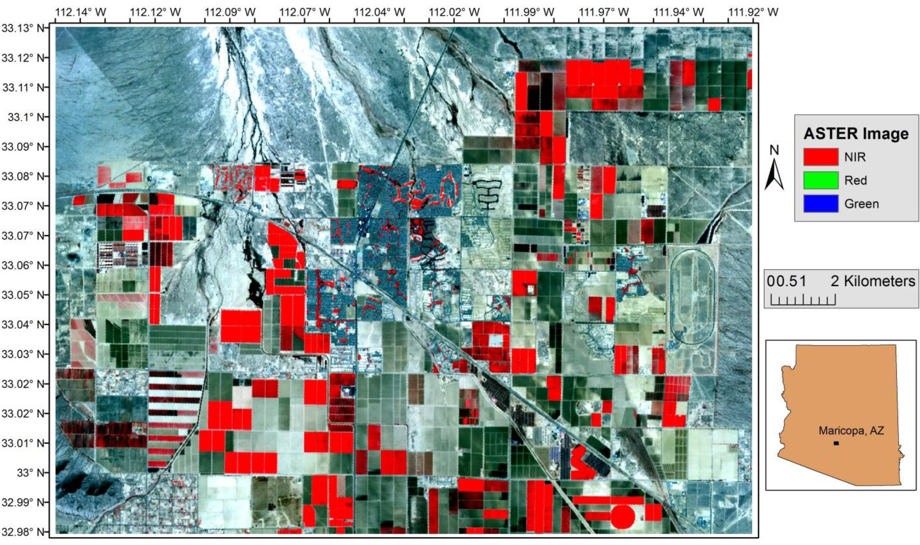
2.1. Data and Study Area

The study area is the city of Maricopa and surrounding landscape in central Arizona. This region represents an intersection of expanding urban development, open desert, and agriculture in the Sun Corridor megapolitan [15], which constitutes a unique land-use dynamic that stretches from Prescott, AZ, to Tucson, AZ and includes Phoenix, AZ. The city of Maricopa has a population of 43,000 as of the 2010 census. Forecasts predict that the population will increase to 47,000 by 2015 [16]. Desert landscapes, part of the Sonoran desert ecosystem, define the natural environment around Maricopa.

The flora of the Sonoran desert (saguaro and prickly pear cactuses, palo verde and mesquite trees, for example) characterizes the hot and dry conditions that persist throughout most of the year. The mean annual temperature is about 21 °C. Mean maximum temperature is about 19 °C in the winter and over 40 °C in the summer. On average, more than 100 days a year exceed 37.7 °C [17]. Annual precipitation is about 280 mm, with half falling in the winter and a quarter falling during the summer monsoon season. The potential evaporation varies by season, but typical conditions reach six times higher than the total precipitation [18].

An ASTER image of the region is the source data for the land-use map. The upper left coordinates of the study area are −112.149859 and 33.125070 decimal degrees and the bottom right are −111.915420 and 32.984877 decimal degrees. The image date is February 27th, 2007, captured at 18:15:27 GMT (Figure 1). ASTER imagery is widely used in both land-use and land cover mapping and with OBIA [19,20]. The visual and near infrared (VNIR) bands and the short wavelength infrared (SWIR) bands were combined into a single image. These bands correspond to ASTER bands one to three in the VNIR range and ASTER bands four through nine in the SWIR range. We selected the ASTER image for our land-use classification to take advantage of the extra SWIR bands, a feature not available in some sensors, especially high resolution imagery where OBIA methods thrive. However, some caution should be taken when using ASTER SWIR data. The ASTER SWIR bands became saturated with noise in 2008 when onboard components vital to capturing the SWIR range failed [21]. All ASTER SWIR images captured before 2008 are still useful for land-use and land cover mapping. To supplement the ASTER bands, we calculated five principle component bands and added them to the image (to improve segmentation and classification). We found the radiometric variability in the image to be sufficient for classification; thus digital numbers were used in lieu of converting the image to top-of-atmosphere reflectance.

Agricultural plots dominate a large portion of the image. Crop species are mostly unknown with the exception of work coinciding with the image date by French et al. [22]. Past evapo-transpiration studies in this study area were conducted on oilseed crops (Camelina sativa), but are not considered to represent a large portion of the agriculture, and cotton cultivars have been produced in the area [23]. The University of Arizona and the USDA Arid Land Agricultural Research Center both operate research facilities in the image boundaries. The study area also includes commercial agriculture and clusters of non-agricultural vegetation in the urban and residential sections—the non-agricultural vegetation is thought to be for recreational use. The city includes a planned area for future housing development, but much of this is currently exposed soil with asphalt pavement running throughout. Many hectares of undeveloped or lightly populated land, comprised of open desert and soil, are interspersed throughout the image. Parts of the Gila River Indian Reservation reside in the northern part of the study area; most of this land is open desert and soil.

The study area offers several classification challenges. Agricultural fields can be confused with open desert, bare soil, or even lightly populated rural areas, mainly because these share common land covers (desert soils). Some areas in the image were marked for development and cleared of all land covers and now expose the underlying soil. This causes confusion between undeveloped plots and open desert, or bare soil. Because these areas will eventually be developed into residential and urban areas, it is inaccurate to classify them as bare soil or open desert. To focus on these challenges, we used a portion of the ASTER image that encompasses the confluence of the confusion between different land-use types.

2.2. OBIA Classification

Land-use was classified with Definiens Developer software [13]. Classifications of objects were based on user-defined decision rules using OBIA. Decision rules are flexibly set by using information from within the image and modified or altered based on the properties of the objects. The decision rules developed in this study were applied to the image over a five-step process. Step one was the image segmentation that formed primitive objects. This was followed in step two by the creation of intermediary classes and spectral analyses of certain objects within these intermediate classes. The third step was an initial classification using the intermediary land-use classes. The fourth step used fusing, morphing, growing, and merging algorithms to improve image segmentation and classify objects based on spatial and spectral information. The fifth step produced a supervised and unsupervised classification for comparison. The last step was the final classification, accuracy assessment, and a diversity assessment used for post-classification modifications. The following sections provide more detail of each methodology step.

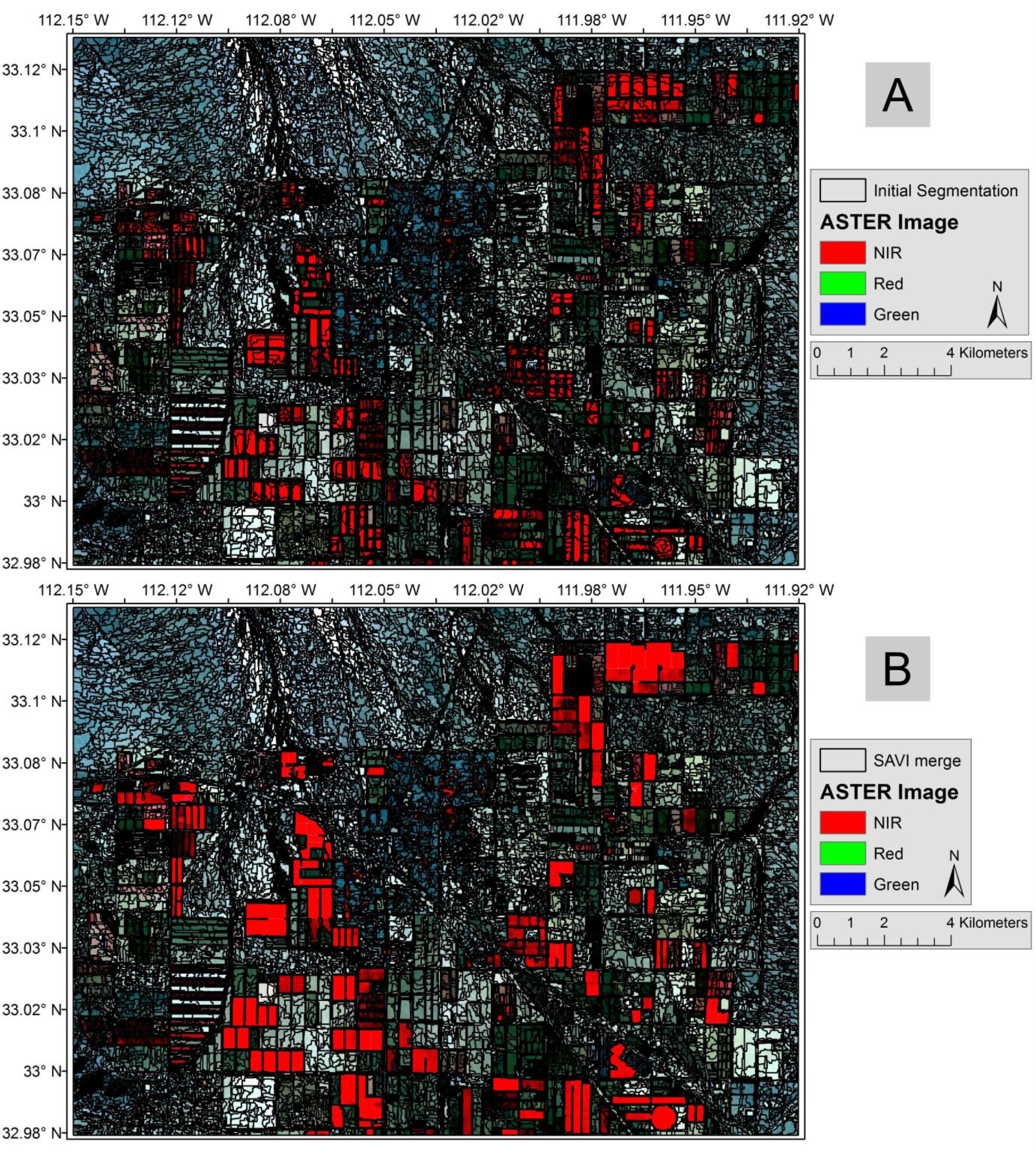
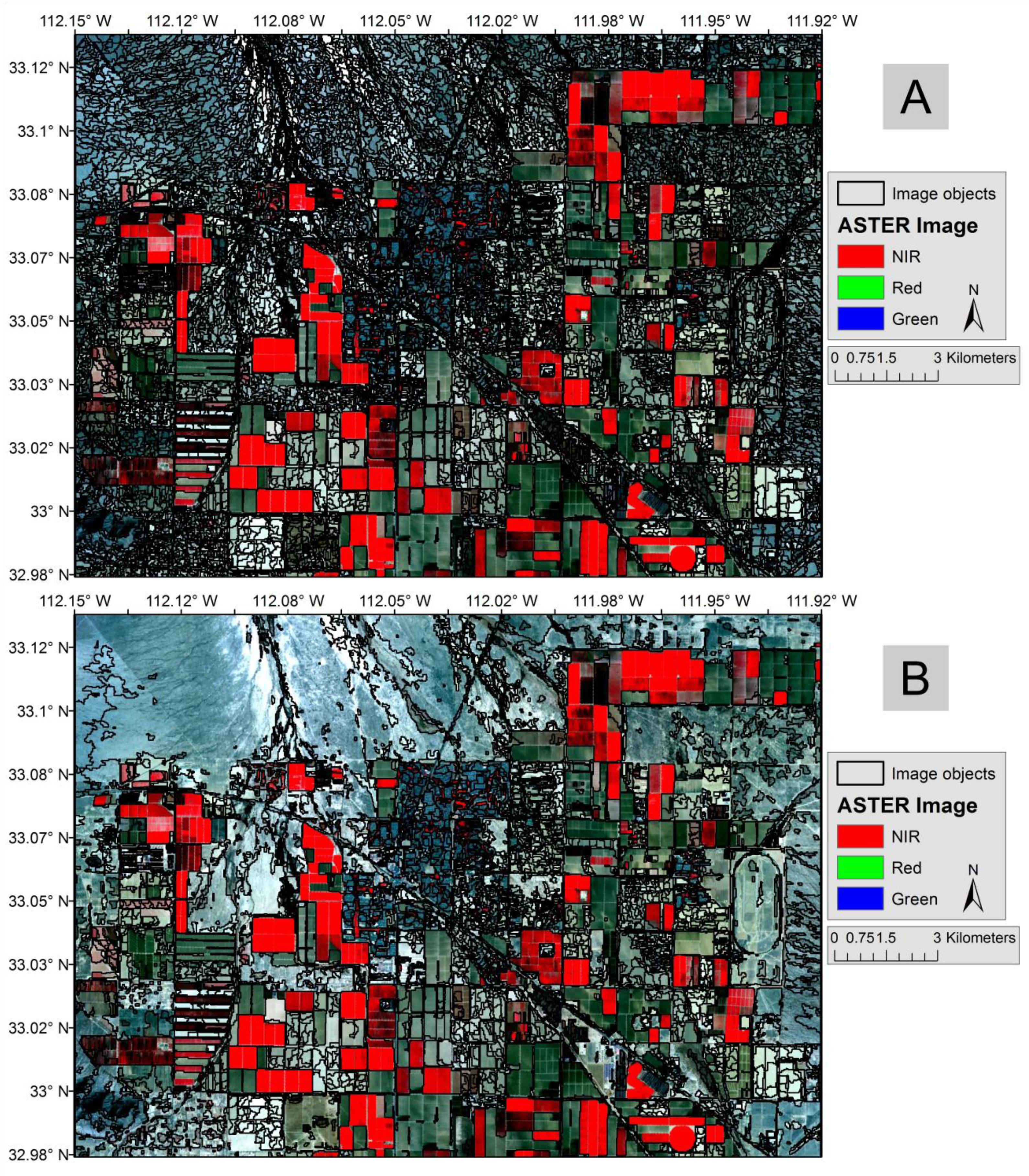
2.2.1. Image Segmentation

The image was segmented with the multiresolution segmentation algorithm in Definiens (Figure 2A) [12]. The scale parameter (an indicator of how big an object is allowed to grow) was set to ten, which produces relatively small objects. Only a single segmentation was performed, which runs counter to most OBIA studies, but has been shown to be effective in land-use classification [24]. After the initial segmentation, a merging algorithm was used to aggregate close to the first and third land-use classes (“active agriculture” and “green space”). The objects to be merged include all that meet specified conditions set in the image object domain [25], which in the case were high SAVI values > 0.7. SAVI is the Soil-Adjusted Vegetation Index [26,27] and is calculated in ASTER images from the following equation:

$$\mathit{SAVI}=\frac{(\mathit{ASTER}3-\mathit{ASTER}2)}{(\mathit{ASTER}3+\mathit{ASTER}2+L)}(1+L)$$

(1)

ASTER3 is the NIR band, ASTER2 is the red band, and L is a soil correction parameter. We set L = 0.5, following other studies done in Arizona [28].

All primitive objects merged using SAVI evolved into aggregate objects, which was used to classify (Figure 2B) either “active agriculture” or “green space” (see Section 2.2.3). In many cases, image segmentation itself can be used to automatically define certain features [29]. In this study, the decision to use a single segmentation and then refine the image objects using merge and grow functions was made based on how well objects coalesced around SAVI (Figure 3) and other spectral properties (Figures 4 and 5).

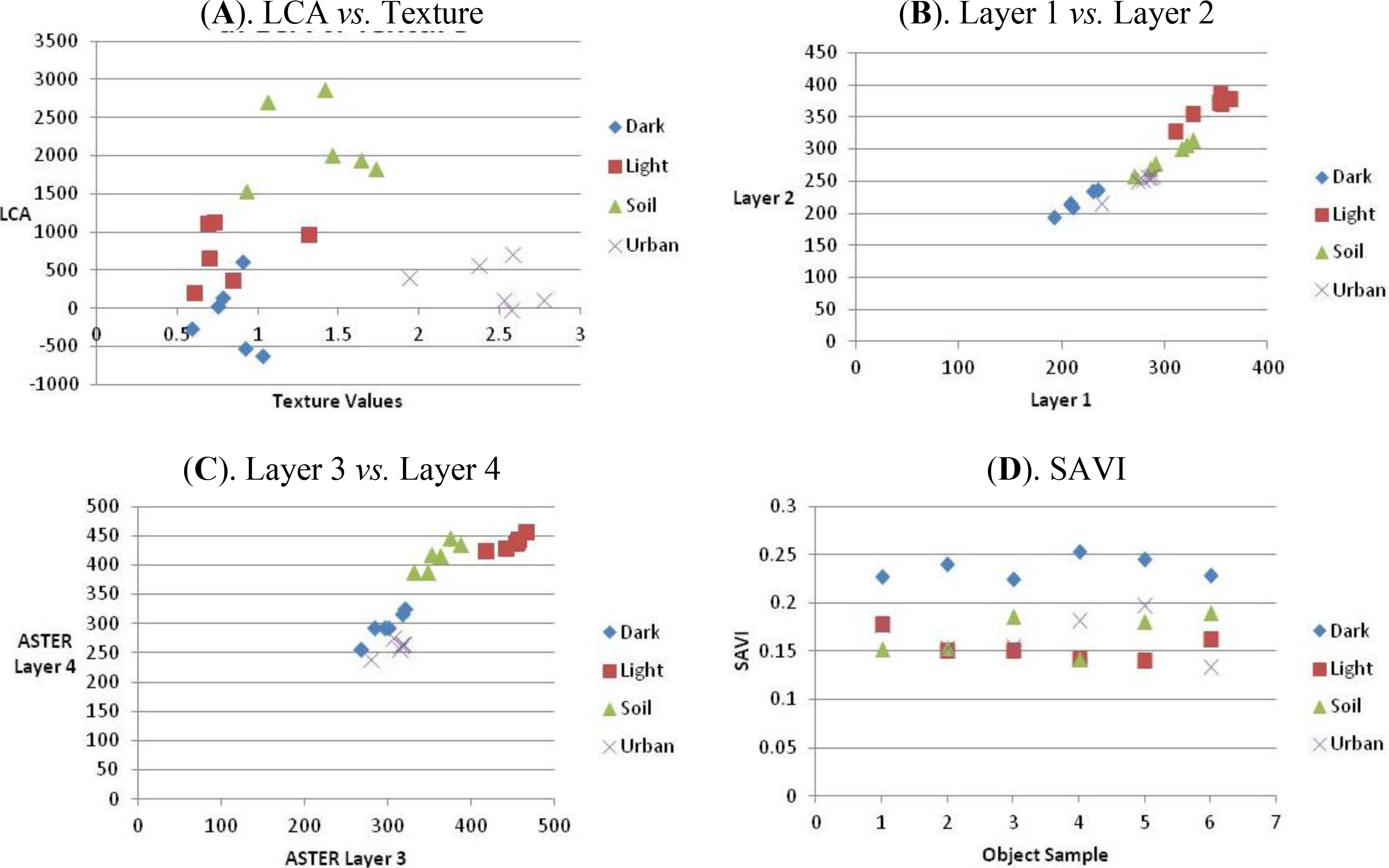
2.2.2. Intermediary Classes and Spectral Evaluation

Fifteen intermediary classes were created to facilitate classification (Table 1). These intermediary classes define different aspects of one or more of the six primary classes. Intermediary classes were also used to aggregate objects (see Section 2.2.4 below) into new objects that better approximate the primary land-use class. Rules were assigned to intermediary classes using analysis of the spectral properties that best differentiated the class.

The spectral evaluation highlighted differences between the rules used for several intermediary classes, especially between: dark agriculture, light/unused agriculture, soil, and urban. Several samples of these four intermediary classes were collected to measure the mean spectral layer values used in decision rules. Six samples of dark inactive agricultural plots (short name: dark), light inactive agricultural plots (short name: light), urban/residential areas (short name: urban), and soil, were graphed using scatter plots. The scatter plots were then reviewed to help visualize and quantify the relationships between LCA (Lignin-Cellulose Absorption) [30–32] and Texture, ASTER layer 1 and 2, ASTER layer 3 and 4, and SAVI (Figure 6). These scatter plots were used to determine cutoffs for different intermediary classes. There were some difficulties in finding meaningful differences between “undeveloped urban,” “open desert,” and “inactive agriculture.” A linear discriminant analysis [33] was performed in SPSS (version 18) to help articulate differences between two intermediary classes: “undeveloped” and light/unused agriculture. The discriminant analysis function developed in SPSS was imported into Definiens and used as a customized feature in the decision rules.

Also during intermediary classification, texture and the LCA index were incorporated to differentiate “inactive agriculture,” “open desert,” “undeveloped urban,” and “developed urban.” Agricultural fields that are not active have low SAVI values and therefore it is not possible to classify solely on SAVI or any other vegetation index. The LCA index has been shown to correlate with agricultural crop litter, so it was incorporated to help classify fields as “inactive agriculture” and to distinguish “inactive agriculture” from “open desert” areas. We found negative and very low positive LCA values to be associated with inactive agriculture, and more positive values to be associated with open desert. Texture, based on the grey-level co-occurrence matrix (GLCM) [34] of standard deviation values from ASTER layer 3, was used to help differentiate inactive agricultural fields from urban areas. Texture and LCA were also used in the discriminant analysis to define “undeveloped urban” areas.

2.2.3. Initial Classification

The first classification was conducted on objects with high SAVI values. After the first round of merging conducted in Section 2.2.1 above, large objects with [SAVI > 0.7] and [Area > 250] were assigned to the “active agriculture” class. Conversely, objects with [Area ≤ 250] and [0.3 < SAVI < 0.9] were assigned to the “non-agriculture vegetation” class. The “non-agriculture vegetation” class was eventually reclassified into the “green space” primary land-use type.

In addition to agriculture, soil and urban areas were also classified in this step. Soil objects were grouped using ASTER layer 3, ASTER layer 4, SAVI, and LCA. Urban areas were classified using GLCM, ASTER Layer 3, ASTER layer 4, and LCA (Figure 7A). Inactive agricultural plots used several intermediary classes for initial classification based on the albedo of the surface, as well as LCA and spatial information.

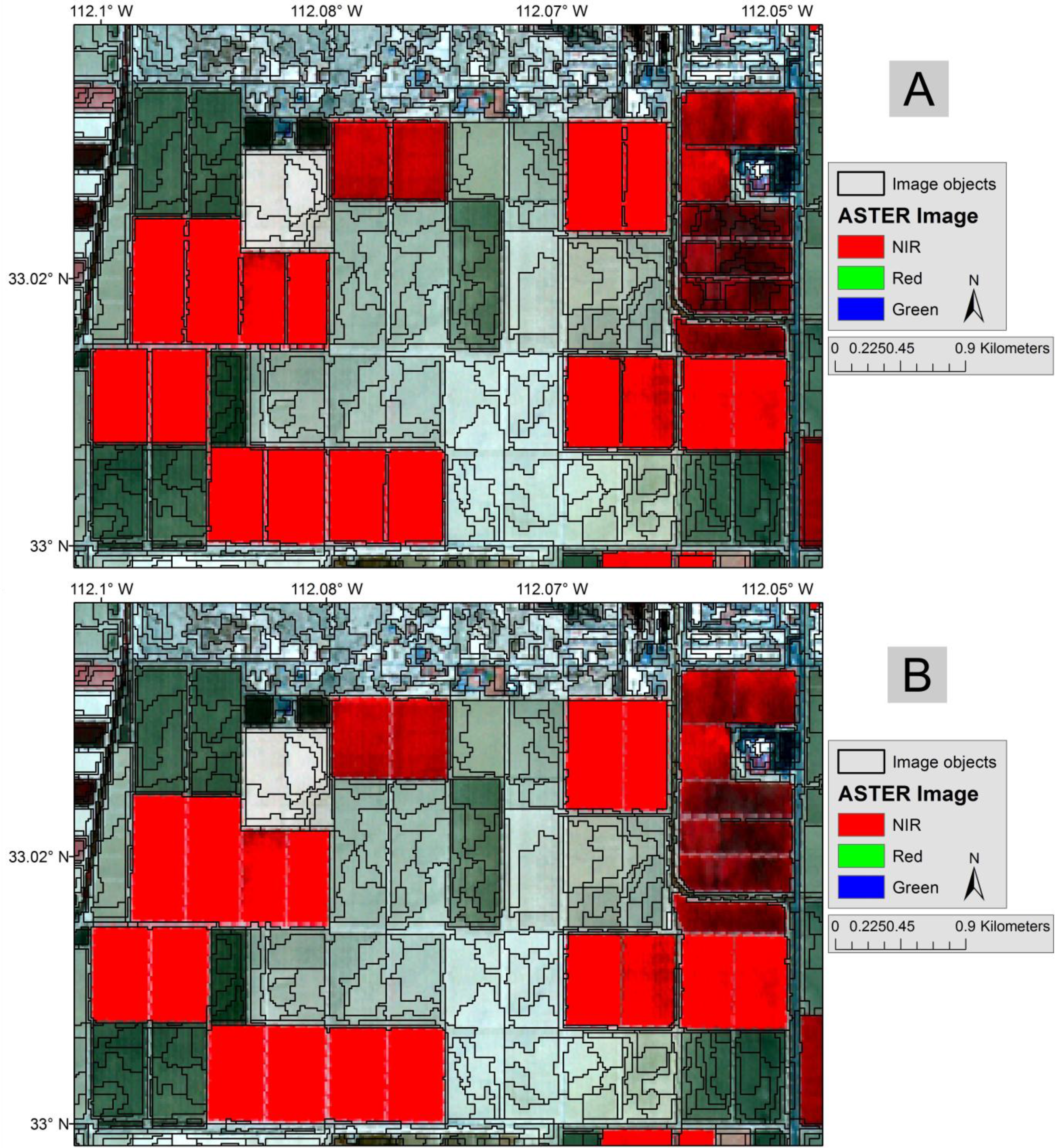
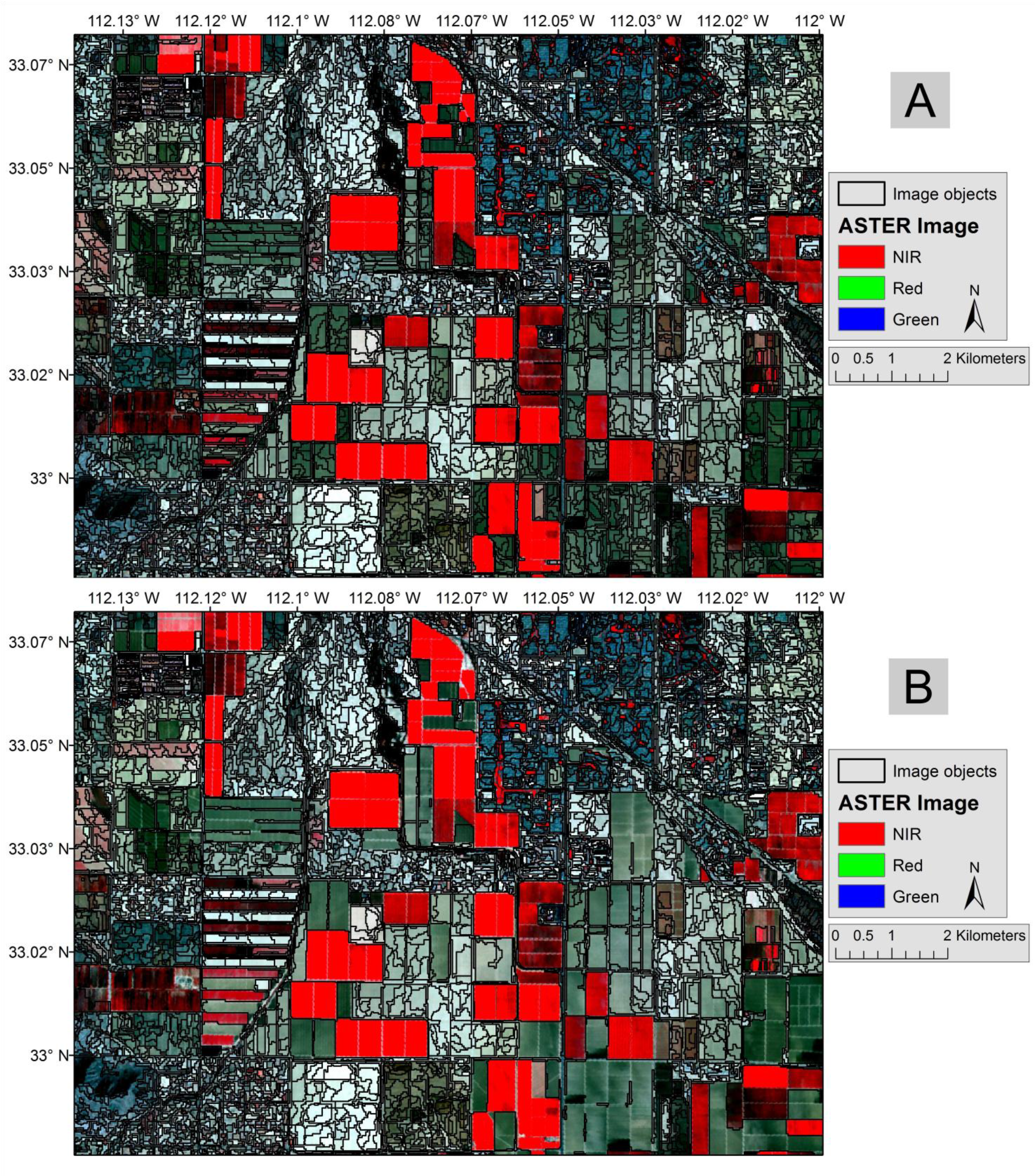
2.2.4. Region Growing, Morphing, and Merging

Despite best efforts at delineating intermediate classes, the initial classification produced results with misclassifications. For example, “open desert” areas were often confused for “inactive agriculture” or “undeveloped urban” (or vice versa). Some “developed urban” objects were misclassified as “undeveloped urban” and “inactive agriculture.” To address the misclassifications, an iterative process of merging, morphing, and growing [25] was performed to help improve the accuracy and take advantage of spatial relationships. The morphology algorithm opens or closes an object based on a user-defined pattern (circle or square) to smooth the border or reshape objects. Opening the object detaches smaller objects around the object’s border. Closing the object in morphology does the opposite by integrating certain bordering objects into the object of interest. The grow region algorithm is similar to the merge region algorithm but differs in that it starts with a seed object defined in the image object domain and grows until some criteria is met. In some cases it was necessary to create a class and then delete it to assist with the modification of objects. By doing this, image objects were morphed, aggregated, and then re-classified until they converged on the proper land-use type (Figure 7B).

One point about this step should be stressed: the process of merging, morphing, or region growing is an iterative step that may also include reclassifications. It is necessary often to assess the outcome of the functions and modify the parameters, sometimes ever so slightly, and then repeat several times. Experimentation was important, and sometimes objects were manipulated to help produce reasonable results. For example, certain objects that were clearly soil, “inactive agriculture,” or “undeveloped urban” required some manual manipulation to keep the process of region growing or merging as seamlessly as possible, but this manipulation was restricted to a small number of objects.

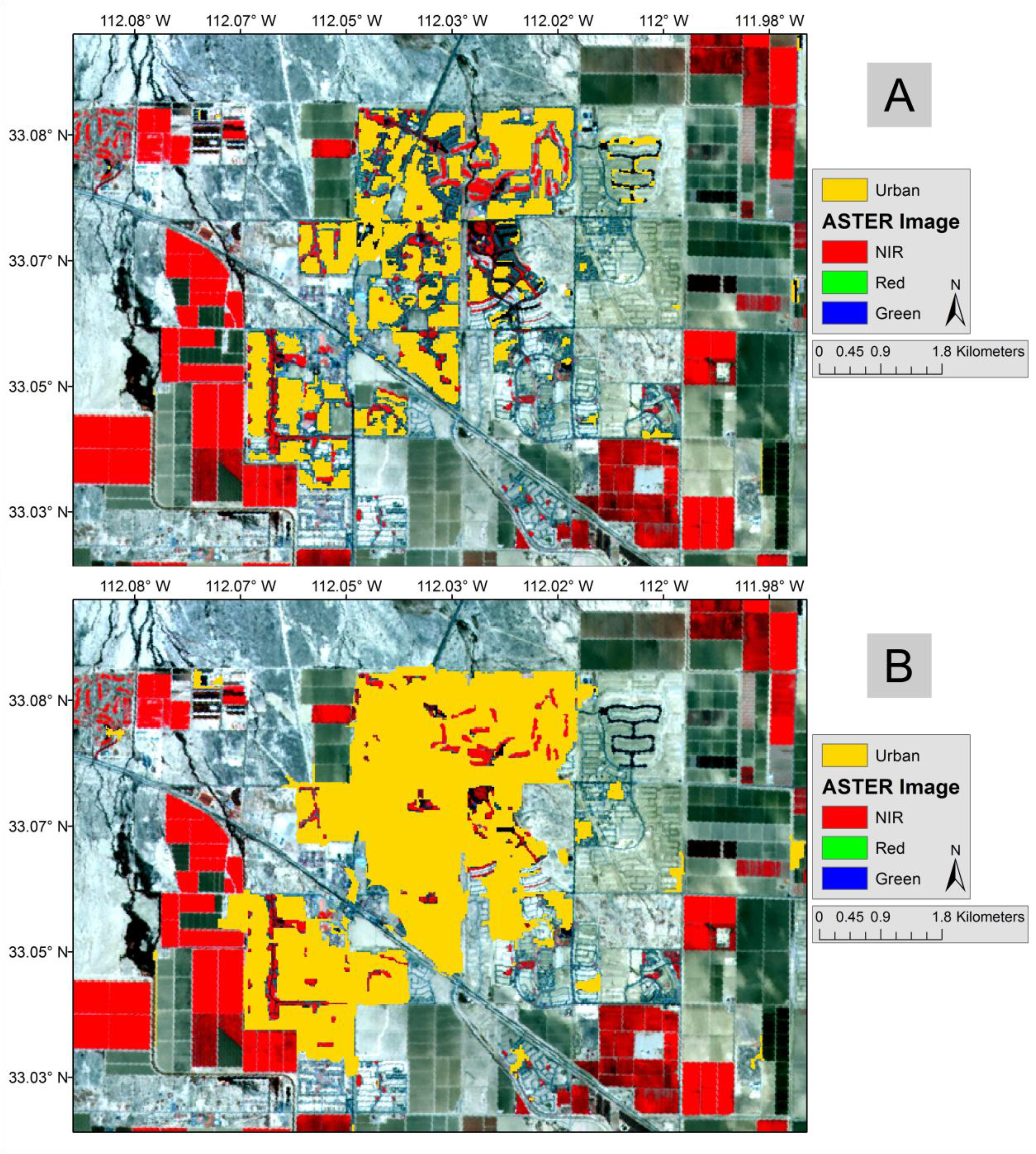
2.2.5. Supervised and Unsupervised Classification

For a better comparison, we employed a supervised and unsupervised classification (Figure 8 and 9) using the ISODATA algorithm [35] to gauge the accuracy of the OBIA land-use map. The unsupervised classification was derived using 30 classes calculated over 10 iterations and a convergence threshold of .95. Each of these classes was then assigned to the same land-use classes as the OBIA classification. Additionally, a maximum likelihood supervised classification was performed. The maximum likelihood classifier has been found to perform as well or better than some OBIA approaches [36]. Only one class was omitted from either classification, “green space,” because it was defined using a spatial property in the OBIA land-use map (area), and there was no meaningful spectral distinction between urban “green space” and agricultural land-use. To keep the comparison as similar as possible, all random points within the unsupervised classification that fell on areas that were known to be green spaces were omitted from the accuracy assessment and a new random point was added in its place. Majority filters were also applied to the unsupervised classification to reduce speckle and improve accuracy (it was also tested for the supervised classification, but did not improve the accuracy).

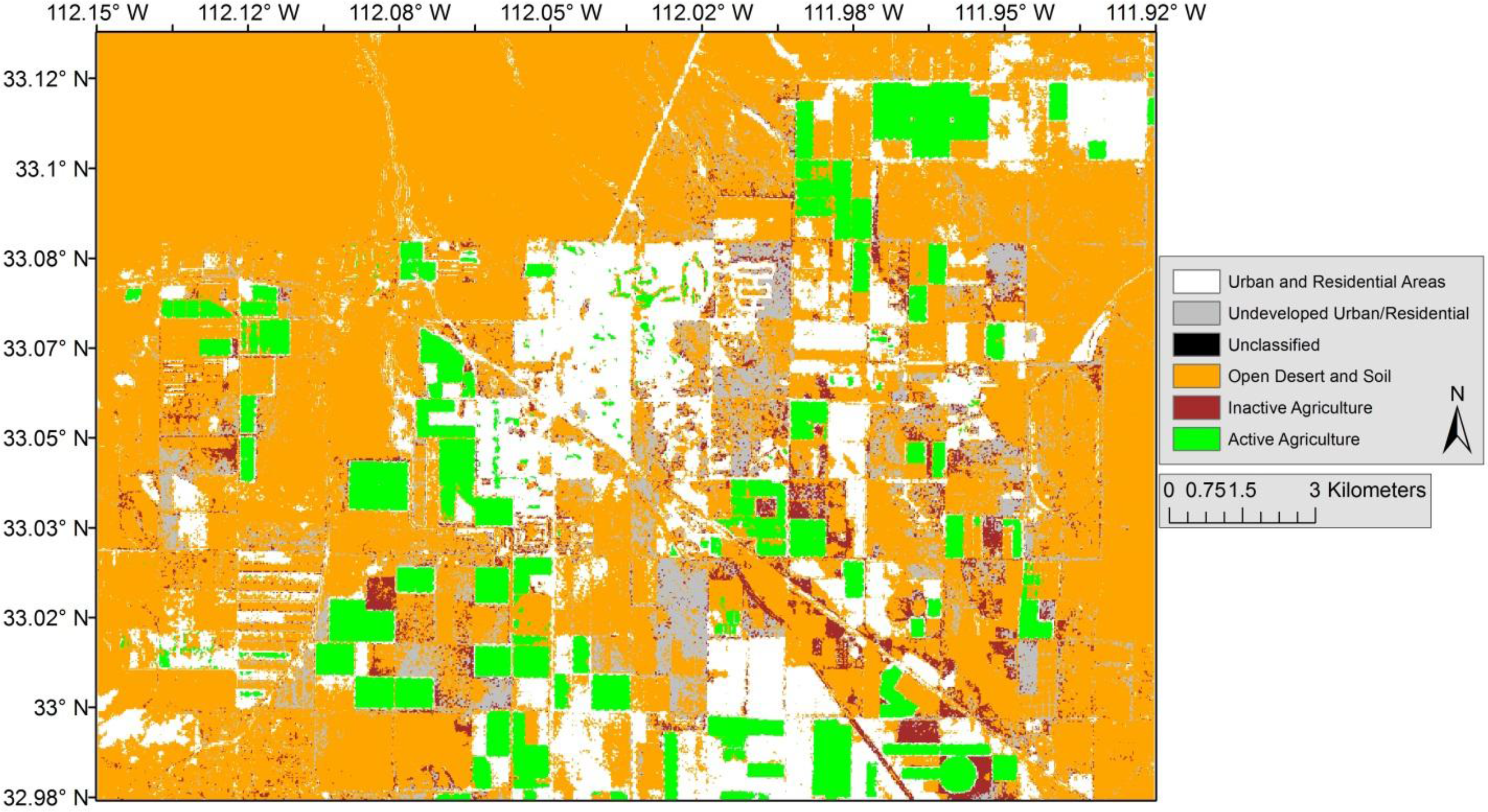
2.2.6. The Final Classification and Assessment

Several more instances of classification, merging, and reclassification occurred in this step. Another Definiens function “find enclosed by” was used for certain objects that were misclassified but clearly surrounded by objects of the correct classification. The “find enclosed by” function will search for any object fully surrounded by a single target class and reclassify it as that target class. The final classification (Figure 10) used ArcGIS to recode the intermediary classes into the six primary land-use classifications.

The accuracy assessment was performed using common methods to remote sensing studies [37,38]. We selected 350 stratified random points with a minimum of 30 random points per class. The same assessment was also performed on the unsupervised classification. For both images, the accuracy of a point was assessed based on expert knowledge of the scene and the region.

The final step was a diversity assessment. Diversity assessments are common in land-use/cover analyses and landscape ecology [39] where a window traverses the entire classified image and records the number of different land-use classes within the window. Window size, as measured in pixels, can vary based on the requirements of the study. Our anticipation was that the OBIA approach would reduce the diversity of land-use types in a given window because of the segmentation process. Conversely, the per-pixel approaches would speckle the image with varying land-use types because it does not consider the spectral information of neighboring pixels. It was hypothesized that the supervised and unsupervised classification will have more land-use classes per moving-window than the OBIA classification. The diversity assessment in this study used a 7 × 7 pixel window to measure the number of different land-use classes per window that is recorded as the value of the center pixel within the window.

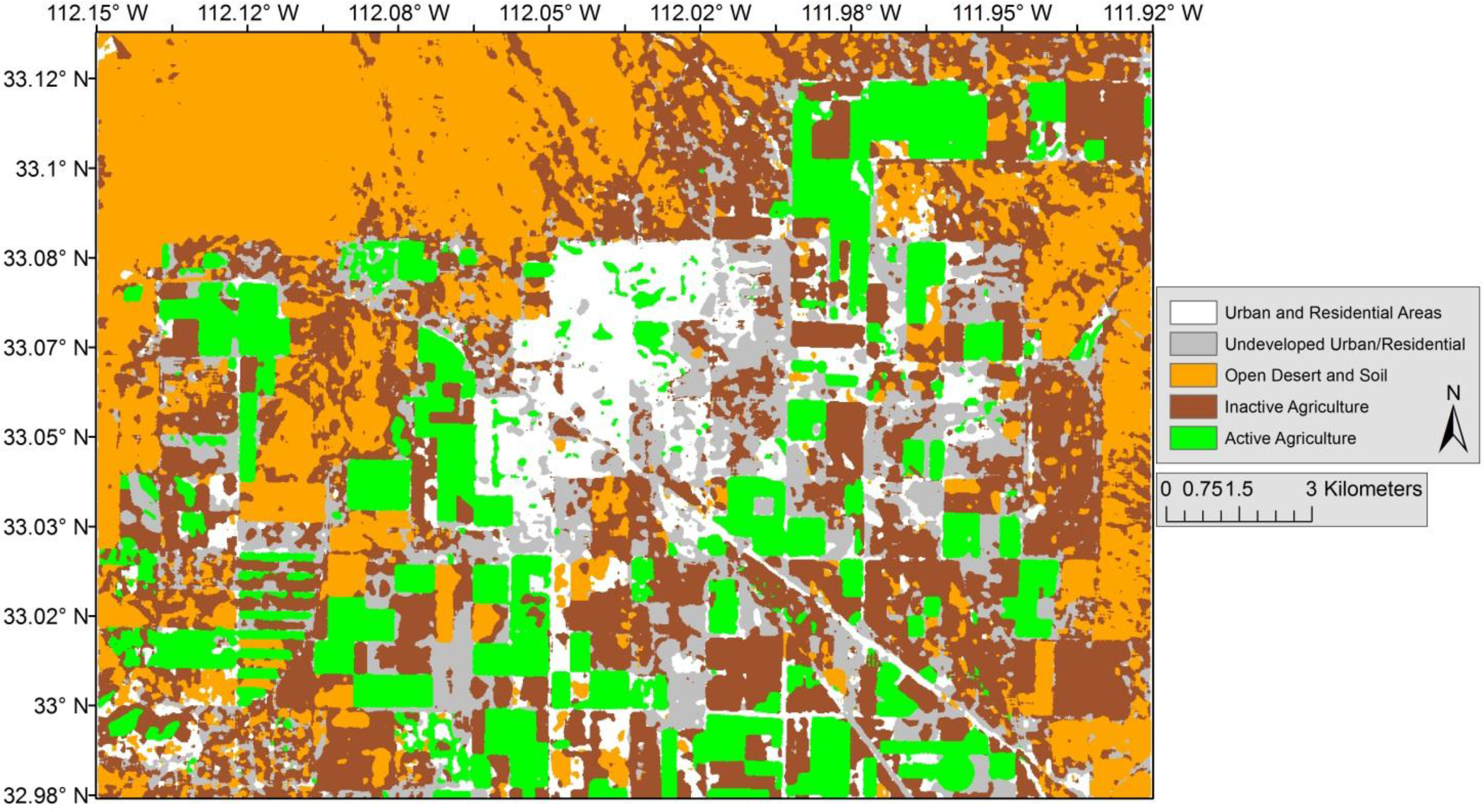
3. Results and Discussion

The results of the accuracy assessment for the OBIA (Figure 10), supervised classification (Figure 8), and unsupervised classification (Figure 9) were compared (

Table 2. Error matrix and classification accuracy—OBIA.

Classified Data	Active Ag.	Inactive Ag.	Green Space	Open Desert	Undevel’d Urban/Res.	Developed Urban/Res	Row Total	Ref. Totals	Class.Totals	# Correct	Prod.’ Accur.	Users’ Accur
Active Ag.	54	0	0	0	0	0	54	67	54	54	80.60%	100.00%
Inactive Ag.	6	68	0	7	0	0	81	73	81	68	93.15%	83.95%
Green Space	7	2	31	0	0	0	40	31	40	31	100.00%	77.50%
Open Desert	0	1	0	88	0	1	90	96	90	88	91.67%	97.78%
Undeveloped Urban/Res.	0	2	0	1	34	6	43	34	43	34	100.00%	79.07%
Developed Urban/Res	0	0	0	0	0	42	42	49	42	42	85.71%	100.00%
Column Totals	67	73	31	96	34	49	350	350	350	317
Overall Accuracy = 90.57%, Overall Kappa = 0.8840

,

Table 3. Error matrix and classification accuracy—Unsupervised Classification.

Classified Data	Active Ag.	Inactive Ag.	Developed Urban/Res	Open Desert	Undeveloped Urban/Res.	Reference Totals	Classified Totals	Number Correct	Producers’ Accuracy	Users’ Accuracy	Row Total
Active Ag.	52	3	0	1	0	60	56	52	86.67%	92.86%	56
Inactive Ag.	2	61	0	42	2	107	107	61	57.01%	57.01%	107
Developed Urban/Res	1	14	15	4	1	20	35	15	75.00%	42.86%	35
Open Desert	1	19	0	83	0	143	103	83	58.04%	80.58%	103
Undeveloped Urban/Res.	4	10	5	13	17	20	49	17	85.00%	34.69%	49
Column Totals	60	107	20	143	20	350	350	228			350
Overall Accuracy = 65.14%, Overall Kappa = 0.5322

, and

Table 4. Error matrix and classification accuracy—Supervised Classification.

Classified Data	Active Ag.	Inactive Ag.	Developed Urban/Res	Open Desert	Undeveloped Urban/Res.	Row Total	Reference Totals	Classified Totals	Number Correct	Producers’ Accuracy	Users’ Accuracy
Active Ag.	43	0	0	0	0	43	55	43	43	78.18%	100.00%
Inactive Ag.	0	26	0	2	2	30	115	30	26	22.61%	86.67%
Developed Urban/Res	4	25	25	12	0	66	28	66	25	89.29%	37.88%
Open Desert	8	46	2	114	4	174	131	174	114	87.02%	65.52%
Undeveloped Urban/Res.	0	18	1	3	15	37	21	37	15	71.43%	40.54%
Column Totals	55	115	28	131	21	350	350	350	223
Overall Accuracy = 63.71%, Overall Kappa = 0.513

). The OBIA method demonstrated higher accuracy than the supervised or unsupervised classification. The overall accuracy of the OBIA land-use map was 90.67%, with a Kappa of 0.8833. The overall accuracy of the unsupervised land-use map was 65.14%, with an overall Kappa of 0.5322. The accuracy of the supervised classification was 63.71%, with a Kappa of 0.513. Unsupervised classifications allocate classes to pixels based on the spectral difference between an arbitrary number of classes (30 for this study), whereas the supervised classification relies on signatures created from samples of different classes. The improved accuracy of the OBIA method over the supervised and unsupervised method is expected based on numerous studies showing that grouping pixels into objects can improve classification performance [14,40]. However, not all studies have demonstrated that OBIA always outperforms per-pixel approaches [36], thus warranting further comparisons.

The unsupervised classification satisfactorily classified “active agriculture” (∼87% producers’ accuracy and ∼93% user’s accuracy), which compares to the OBIA method (∼81% producer’s and 100% user’s) and the supervised classification (78% producer’s and 100% user’s). The spectral properties of the vegetation make it easy to distinguish “active agriculture” from other land-use types. The morphing, merging, and growing of image objects, as well as using the size of the objects, helped to delineate “active agriculture” from other types of land uses in the OBIA method. It is possible in other study areas that agriculture may not be defined by size (e.g., small urban farm plots). If this is the case, other spatial information or geometry could assist in classifying agriculture. Shape parameters may help alleviate this problem, and could be an area for future exploration. Agriculture is distinctly square or circular in most applications; this characteristic could be exploited to automate classification of agriculture, no matter the size of the plots.

The classification of fallow or dormant agricultural plots (“inactive agriculture”) was difficult because these were spectrally similar qualities to other land uses. The accuracy assessment of the inactive agricultural plots is different between the OBIA method and the supervised and unsupervised classification (93% producers and 84% users for OBIA, 22% producer’s and 86% user’s for supervised, and 57% producers and 57% users for the unsupervised classification). The reason for such a disparity between these three methods is that the spectral properties of inactive agricultural plots are similar to “open desert” and “undeveloped urban.” The “open desert” class overlapped with “inactive agriculture” in the unsupervised and supervised classifications. The LCA index helped to distinguish fallow agriculture from open desert, as well as the discriminant analysis, but the OBIA also had the advantage of creating distinct objects—using the merging and growing object functions—which helped delineate large “open desert” and “inactive agriculture” plots.

The classification of “developed urban” varied widely between the OBIA and unsupervised classification method. The unsupervised classification had a producers’ accuracy of 75% and a users’ accuracy of 43%, whereas the OBIA accuracy for “developed urban” was 86% for the producer’s accuracy and had a users’ accuracy of 100%. The OBIA classification utilized several properties to distinguish the urban areas from other classes, including a PCA band (PCA 1), LCA, and texture, which both LCA and texture had excellent discrimination from other spectrally similar classes (Figure 4).

The “undeveloped urban” classification varied in results between the OBIA and unsupervised classification methods. The OBIA method had a 100% producer’s accuracy and 79% user’s accuracy, whereas the unsupervised classification had an 85% producer’s and 34% user’s accuracy. While the OBIA method more accurately classified “undeveloped urban,” there were still problems separating it from “open desert,” “inactive agriculture.” The spectral similarities between these three classes are the result of similar land covers (bare soil/sediment). The discriminant analysis helped classify the undeveloped areas, but only after the undeveloped areas were already classified using the “light/unused agriculture” intermediary class. It took several instances of classifying, reclassifying, and merging objects with intermediary classes to finally articulate the “undeveloped urban” land-use class in the final classification. However, as the user’s accuracy shows, there were several areas that were clearly “undeveloped urban” but were still misclassified as “open desert” or “inactive agriculture.” One observation noted in this study that has also been noted by others [7,24] is that land-use maps are capable of being produced from within the image data; however, confusion often occurs among land-use classes when similar land cover types are common between the classes. To reduce the impact of this problem, multiple steps of experimentation and refinement were performed during the development of the decision rules.

The diversity assessment indicates the amount of heterogeneity of the classified image (

Table 5. Diversity assessment results.

	Unsupervised		Supervised		OBIA
Classes per 7 ×7 pixel window	Window count	Windows times classes	Window count	Windows times classes	Window count	Windows times classes
1 class	552,488	552,488	504,954	504,954	893,234	893,234
2 classes	443,938	887,876	340,562	681,124	233,997	467,994
3 classes	160,944	482,832	230,895	692,685	54,006	162,018
4 classes	29,512	118,048	101,643	406,572	6,672	26,688
5 classes	1,658	8290	10,486	52,430	622	3,110
6 classes	0	0	0	0	9	54
Sum:	1,188,540	2,049,534	1,188,540	2,337,765	1,188,540	1,553,098

). On a per-window basis, the OBIA classified fewer land use classes in any given 7 × 7 window vs. the unsupervised or supervised classification. This confirmed our initial hypothesis (Section 2.6) and agrees with other studies comparing per-pixel classification methods with OBIA approaches [36,40]. This does not allude to the overall accuracy of the image; rather, it should be used to measure the amount of effort required for post-classification modification. The OBIA method has a higher concentration of windows with one land-use class, denoting a certain level of contiguity in the classification (Figure 11). For OBIA, there is a lower frequency of windows as the number of land-use classes increases, following an exponentially decaying trend. The supervised and unsupervised classifications decay more linearly, which is indicative of these classifications being based solely on the spectral qualities of a single pixel. We believe this is the result of the segmentation and grouping of pixels into objects. The segmentation process uses spatial relationships in a way that is not possible with per-pixel approaches [13], which is something that can be easily overlooked [36].

The information gained from the diversity assessment highlights potential misclassifications, and serves as a guide for modifications to the classified map, similar to decision support systems used in other studies [7]. Windows of pixels with one, two, or even three classes may be common, but a high number of classes per window can signal misclassified pixels. In a follow up to the diversity assessment, the land-use map was manually modified using the diversity assessment as a guide. The overall accuracy of the image was increased to 93.71% and the Kappa increased to 0.9223. The diversity assessment improved the classification by focusing on areas of greater heterogeneity.

4. Conclusions

A step-by-step procedure was given to map land-use in a mixed urban/agricultural area with ASTER imagery and object-based image analysis (OBIA). We demonstrated that it was possible to use a single multi-resolution segmentation of an ASTER image with a scale parameter of 10 to form meaningful objects. Two algorithms, grow region and merge region, transformed primitive objects into objects of interest. We classified active agriculture by merging all objects with a soil-adjusted vegetation index (SAVI) higher than 0.7, and then grew the region around it with slightly lower SAVI values. Similar methods were used to classify inactive agriculture (or fallow fields) and urban areas. Once the objects were formed, spatial information, such as area and relative distance, were used to classify the objects. Our research reinforces that object geometry and spatial relationships are effective when spectral properties alone are not sufficient to differentiate classes.

The Lignin-Cellulose Absorption index proved to be helpful both for classifying fallow fields and uncovering differences between fallow agricultural fields and open desert. Negative or weakly positive LCA values were associated with inactive agricultural fields, while deserts were associated with higher positive values. Land-use classifications that need to differentiate between open desert areas and inactive agricultural plots should consider the LCA (or a similar index) to help differentiate these two classes. An alternative is to use multi-temporal imagery to solve the confusion between fallow (inactive) agriculture and open desert, and this will be pursued in future research.

We also demonstrated that a land-use diversity assessment can assist the improvement of the final classification. The diversity assessment flags areas of high land-use heterogeneity, and we used these high diversity areas as a way to improve the final land-use map. This technique can be used to identify areas that need improvement, either for post-classification modifications or to refine the decisions rules. We also found that the OBIA method generates fewer regions of high land-use heterogeneity, which corroborates other research.

Finally, much of the focus of OBIA research centers on high resolution imagery, and OBIA seems to be used overwhelmingly to map land cover. Based on the outcome of this study, classifications using imagery from moderate resolution sensors (like ASTER) can also benefit from OBIA—and it need not be used solely for land-cover mapping. Meaningful land-use maps are possible, too, because while the land-use classes may be scale dependent, the methods are not.

References

1. Seto, K.C.; Fragkias, M.; Güneralp, B.; Reilly, M.K. A meta-analysis of global urban land expansion. PLoS ONE 2011, 6, e23777. [Google Scholar]
2. Population Reference Bureau, 2011 World Population Data Sheet; Population Reference Bureau: Washington, DC, USA, 2011; pp. 1–5.
3. Meyer, W.B.; Turner, B.L., II. Human-population growth and global land-use cover change. Annu. Rev. Ecol. Syst 1992, 23, 39–61. [Google Scholar]
4. Foley, J.A.; DeFries, R.; Asner, G.P.; Barford, C.; Bonan, G.; Carpenter, S.R.; Chapin, F.S.; Coe, M.T.; Daily, G.C.; Gibbs, H.K.; et al. Global consequences of land use. Science 2005, 309, 570–574. [Google Scholar]
5. Reynolds, J.F.; Smith, D.M.S.; Lambin, E.F.; Turner, B.L., II; Mortimore, M.; Batterbury, S.P.J.; Downing, T.E.; Dowlatabadi, H.; Fernández, R.J.; Herrick, J.E.; et al. Global desertification: Building a science for dryland development. Science 2007, 316, 847–851. [Google Scholar]
6. Turner, B.L., II; Lambin, E.F.; Reenberg, A. The emergence of land change science for global environmental change and sustainability. Proc. Natl. Acad. Sci. USA 2007, 104, 20666–20671. [Google Scholar]
7. Rozenstein, O.; Karnieli, A. Comparison of methods for land-use classification incorporating remote sensing and GIS inputs. Appl. Geogr 2011, 31, 533–544. [Google Scholar]
8. Lu, D.; Weng, Q. Use of impervious surface in urban land-use classification. Remote Sens. Environ 2006, 102, 146–160. [Google Scholar]
9. Blaschke, T. Object based image analysis for remote sensing. ISPRS J. Photogramm. Remote Sens 2010, 65, 2–16. [Google Scholar]
10. Blaschke, T.; Hay, G.J.; Kelly, M.; Lang, S.; Hofmann, P.; Addink, E.; Feitosa, R.Q.; van der Meer, F.; van der Werff, H.; van Coillie, F.; Tiede, D. Geographic Object-Based Image Analysis—Towards a new paradigm. ISPRS J. Photogramm. Remote Sens 2014, 87, 180–191. [Google Scholar]
11. Blaschke, T.; Hay, G. J.; Weng, Q.; Resch, B. Collective sensing: Integrating geospatial technologies to understand urban systems—An overview. Remote Sens 2011, 3, 1743–1776. [Google Scholar]
12. Baatz, M.; Schape, A. Multiresolution Segmentation: An Optimization Approach for High Quality Multi-Scale Image Segmentation. In Angewandte Geographische Informationsverarbeitung XII; Strobl, J., Blaschke, T., Griesebner, G., Eds.; Wichmann Verlag: Karlsruhe, Germany, 2000; pp. 12–23. [Google Scholar]
13. Benz, U.; Hofmann, P.; Willhauck, G.; Lingenfelder, I.; Heynen, M. Multi-resolution, object-oriented fuzzy analysis of remote sensing data for GIS-ready information. ISPRS J. Photogramm. Remote Sens 2004, 58, 239–258. [Google Scholar]
14. Myint, S.W.; Gober, P.; Brazel, A.; Grossman-Clarke, S.; Weng, Q. Per-pixel vs. object-based classification of urban land cover extraction using high spatial resolution imagery. Remote Sens. Environ 2011, 115, 1145–1161. [Google Scholar]
15. Grimm, N.B.; Foster, D.; Groffman, P.; Grove, J.M.; Hopkinson, C.S.; Nadelhoffer, K.J.; Pataki, D.E.; Peters, D.P. The changing landscape: Ecosystem responses to urbanization and pollution across climatic and societal gradients. Front. Ecol. Environ 2008, 6, 264–272. [Google Scholar]
16. City of Maricopa. Size and Location. Available online: http://www.maricopa-az.gov/web/visiting-maricopa/population-demographics (accessed on 25 February 2014).
17. Hartz, D.A.; Brazel, A.J.; Golden, J.S. A comparative climate analysis of heat-related emergency 911 dispatches: Chicago, Illinois and Phoenix, Arizona USA 2003 to 2006. Int. J. Biometeorol 2013, 57, 669–678. [Google Scholar]
18. Balling, R.C.; Gober, P. Climate variability and residential water use in the city of Phoenix, Arizona. J. Appl. Meteorol. Climatol 2007, 46, 1130–1137. [Google Scholar]
19. Chen, Y.; Shi, P.; Fung, T.; Wang, J.; Li, X. Object-oriented classification for urban land cover mapping with ASTER imagery. Int. J. Remote Sens 2007, 28, 4645–4651. [Google Scholar]
20. Crocetto, N.; Tarantino, E. A class-oriented strategy for features extraction from multidate ASTER imagery. Remote Sens 2009, 1, 1171–1189. [Google Scholar]
21. NASA Jet Propulsion Laboratory. SWIR—ASTER User Advisory. Available online: http://asterweb.jpl.nasa.gov/swir-alert.asp (accessed on 5 October 2011).
22. French, A.N.; Hunsaker, D.; Thorp, K.; Clarke, T. Evapotranspiration over a camelina crop at Maricopa, Arizona. Ind. Crop. Prod 2009, 29, 289–300. [Google Scholar]
23. Mauney, J.R.; Kimball, B.A.; Pinter, P.J., Jr.; LaMorte, R.L.; Lewin, K.F.; Nagy, J.; Hendrey, G.R. Growth and yield of cotton in response to a free-air carbon dioxide enrichment (FACE) environment. Agric. Forest Meteorol. 1994, 70, 49–67. [Google Scholar]
24. Lang, S.; Langanke, T. Object-based mapping and object-relationship modeling for land use classes and habitats. Photogramm. Fernerkun 2006, 2006, 5–18. [Google Scholar]
25. Definiens, AG. eCognition Developer 8 User Guide; Definiens AG: Munich, Germany, 2009; pp. 170–171. [Google Scholar]
26. Huete, A.R. A soil-adjusted vegetation index (SAVI). Remote Sens. Environ 1988, 25, 295–309. [Google Scholar]
27. Qi, J.; Chehbouni, A.; Huete, A.R.; Kerr, Y.H.; Sorooshian, S. A modified soil adjusted vegetation index. Remote Sens. Environ 1994, 48, 119–126. [Google Scholar]
28. Stefanov, W.L.; Ramsey, M.S.; Christensen, P.R. Monitoring urban land cover change: An expert system approach to land cover classification of semiarid to arid urban centers. Remote Sens. Environ 2001, 77, 173–185. [Google Scholar]
29. Dragut, L.; Blaschke, T. Automated classification of landform elements using object-based image analysis. Geomorphology 2006, 81, 330–344. [Google Scholar]
30. Daughtry, C.S.T.; Doroiswamy, P.C.; McMurtrey, J.E., III. Remote sensing the spatial distribution of crop residues. Agron. J 2005, 97, 864–871. [Google Scholar]
31. Serbin, G.; Daughtry, C.S.T.; Huntjr, E.R., Jr.; Reeves, J.B., III; Brown, D.J. Effects of soil composition and mineralogy on remote sensing of crop residue cover. Remote Sens. Environ 2009, 113, 224–238. [Google Scholar]
32. Daughtry, C.S.T.; Serbin, G.; Reeves, J.B., III; Doraiswamy, P.C.; Hunt, E.R., Jr. Spectral reflectance of wheat residue during decomposition and remotely sensed estimates of residue cover. Remote Sens 2010, 2, 416–431. [Google Scholar]
33. Myint, S.W.; Lam, N. A study of lacunarity-based texture analysis approaches to improve urban image classification. Compute. Environ. Urban Syst 2005, 29, 501–523. [Google Scholar]
34. Haralick, R.M.; Dinstein, I.; Shanmugam, K. Textural features for image classification. IEEE T. Syst. Man Cyb 1973, 3, 610–621. [Google Scholar]
35. Ball, G.H.; Hall, D.J. A clustering technique for summarizing multivariate data. Behav. Sci 1967, 12, 153–155. [Google Scholar]
36. Myint, S.W.; Galletti, C.S.; Kaplan, S.; Kim, W.Y. Object vs. pixel: A systematic evaluation in urban environments. Geocarto Int 2013, 28, 657–678. [Google Scholar]
37. Congalton, R.G. A review of assessing the accuracy of classifications of remotely sensed data. Remote Sens. Environ 1991, 37, 35–46. [Google Scholar]
38. Foody, G.M. Status of land cover classification accuracy assessment. Remote Sens. Environ 2002, 80, 185–201. [Google Scholar]
39. Turner, M.G.; Gardner, R.H.; O’Neill, R.V. Landscape Ecology in Theory and Practice: Pattern and Process; Springer-Verlag: Berlin/Heidelberg, Germany, 2001; p. 110. [Google Scholar]
40. Yuan, F.; Bauer, M.E. Mapping Impervious Surface Area Using High Resolution Imagery: A Comparison of Object-Based and Per Pixel Classification. Proceedings of American Society for Photogrammetry and Remote Sensing Annual Conference 2006, Reno, NV, USA, 1–5 May 2006.
Figure 1. ASTER image of the study area in Maricopa, Arizona.
Remotesensing 06 06089f1
Figure 2. (A) Image segmentation using scale parameter of 10. (B) New objects after merging those objects with SAVI > 0.7.
Remotesensing 06 06089f2
Figure 3. (A) Detail of objects formed after merging those with mean SAVI > 0.7. (B) After morphing and growing objects of SAVI > 0.5.
Remotesensing 06 06089f3
Figure 4. Comparison of objects before (A) and after (B) a merge of very low LCA.
Remotesensing 06 06089f4
Figure 5. Comparison of objects before (A) and after (B) a merge of high LCA.
Remotesensing 06 06089f5
Figure 6. Scatter plots showing similarities and differences between four intermediary classes. (A) LCA vs. Texture; (B) Layer 1 vs. Layer 2; (C) Layer 3 vs. Layer 4 and (D) SAVI.
Remotesensing 06 06089f6
Figure 7. (A) Initial classification of urban land-use. (B) Intermediary urban land-use after “grow region” and merging of objects.
Remotesensing 06 06089f7
Figure 8. Supervised land-use classification.
Remotesensing 06 06089f8
Figure 9. Unsupervised land-use classification (with majority filter).
Remotesensing 06 06089f9
Figure 10. The OBIA land-use classification.
Remotesensing 06 06089f10
Figure 11. Diversity summary—number of land-use classes per moving window.
Remotesensing 06 06089f11