Article

Improved van Zyl Polarimetric Decomposition Lessening the Overestimation of Volume Scattering Power

1
State Key Laboratory of Information Engineering in Surveying, Mapping and Remote Sensing, Wuhan University, 129 Luoyu Road, Wuhan, Hubei 430079, China
2
Department of Geographical Sciences, University of Maryland, College Park, MD 20742, USA
*
Author to whom correspondence should be addressed.
Remote Sens. 2014, 6(7), 6365-6385; https://doi.org/10.3390/rs6076365
Submission received: 30 April 2014 / Revised: 19 June 2014 / Accepted: 27 June 2014 / Published: 8 July 2014

Abstract

:
This paper improves van Zyl’s Nonnegative Eigenvalue Decomposition (NNED). Orientation angle compensation and helix scattering are introduced to the decomposition. The volume scattering parameters that explain the most cross-polarized power are selected. If volume scattering and helix scattering explain all cross-polarized power in the measured coherency matrix, then simply perform van Zyl decomposition to the remainder matrix; otherwise, the measured coherency matrix is decomposed into three components, i.e., helix scattering, volume scattering, and one ground scattering. The latter two scattering are all modeled by Neumann’s adaptive depolarizing model, according to which some cross-polarized power is attributed to ground scattering hence the orientation angle randomness of volume scattering and the dominant ground scattering are obtained. In this way, all cross-polarized power could be well explained. Experiments using UAVSAR data showed that more than 99.8% of total pixels are well fitted. Negative power is avoided. Compared with van Zyl decomposition, volume scattering power is reduced by up to 8.73% on average. The given volume scattering power is often lower than that by three latest NNED.

1. Introduction

In the field of polarimetric Synthetic Aperture Radar (PolSAR), model-based incoherent decomposition is an important research topic [1]. Since Freeman and Durden proposed the three-component decomposition in 1992 [2] and 1998 [3], more than 20 decompositions have been published [416]. Model-based decomposition has been successfully used in PolSAR image classification [1721], speckle filtering [22], polarimetric SAR Interferometry [23], wetland research [24], soil moisture and roughness estimation [2527], target detection [28,29], disaster assessment [30], and so on. In the past several years, the largest advances include adaptive scattering models [16,26,31,32], Orientation Angle Compensation (OAC) [33], Nonnegative Eigenvalue Constraint (NNEC) [7], etc.
van Zyl et al. [7] demonstrated that if model-based decomposition is valid, then after subtracting any components from the observed covariance or coherency matrix, the remainder matrix must be positive semidefinite, or its eigenvalues must be nonnegative. This constraint is named as NNEC. It could be easily proved that, usually, the decomposition results satisfy NNEC as long as the obtained component powers are nonnegative. In [8,15], NNEC was adopted to eliminate negative power as much as possible. In recent years, several Nonnegative Eigenvalue Decompositions (NNED) were proposed by van Zyl et al. [7], Arii et al. [6], Cui et al. [12], and Wang et al. [13]. In all NNED, the maximum volume scattering power that makes the remainder matrix positive semidefinite is thought to be optimal and selected. In this way, the overestimation of volume scattering power in Yamaguchi decomposition or Freeman-Durden decomposition is largely eliminated. In addition, negative power is fundamentally avoided.
However, NNED still has two potential problems. The first problem is the overestimation of volume scattering power is not entirely eliminated. Since the maximum volume scattering power in theory is adopted, the overestimation is inevitable to a large degree. When applying adaptive volume scattering models, the overestimation is more serious [6,13].
The second problem is how to explain cross-polarized power. Subject to the Reflection Symmetry Assumption (RSA) and employment of elemental scatterers of which cross-polarized complex scattering coefficient, or SHV is zero, the derived coherent models of surface scattering and double-bounce scattering cannot describe depolarizing effect. However, it was observed [7] that if volume scattering power is computed with RSA, then, in many natural forest pixels, volume scattering and helix scattering cannot explain all cross-polarized power. van Zyl attributed these unexplained cross-polarized power to a remainder component which is thought to represent terrain effects and rough surface scattering. If volume scattering power is computed without RSA, then in almost every pixel, volume scattering and helix scattering cannot explain all cross-polarized power. Wang et al. [13] and Cui et al. [12] utilized elemental scatterers of which SHV is non-zero and coherent models, to explain these remaining cross-polarized power. Unfortunately, among all widely recognized scattering mechanisms, only helix scattering with standard orientation has non-zero SHV.
Some researchers may argue that there are possibly some unknown scattering mechanisms, which could produce cross-polarized power. However, according to the latest incoherent adaptive scattering models, such as X-Bragg model [26], Arii’s model [31], and Neumann’s model [32], when the orientation angles of scatterers in one component are not exactly the same, this component will give cross-polarized power as long as SHH + SVV ≠ 0, where SHH and SVV are the complex scattering coefficients, HH means horizontal transmitting and horizontal receiving, VV means vertical transmitting and vertical receiving.
Generally, in incoherent scattering, the assumption that orientation angles in one component are the same cannot be guaranteed even for man-made targets, let alone for natural distributed targets. Natural terrain, like the ground in old-growth forest, is usually rough even when the wavelength is long. Hence, surface scattering could produce non-zero cross-polarized power. Similarly, double-bounce scattering with cross-polarized power also widely distribute in natural environment. From this perspective, both surface scattering and double-bounce scattering could give cross-polarized power in incoherent scattering. Neumann [32] found that in forest, ground scattering has significant cross-polarized power. Therefore, it is wiser to apply incoherent models for ground scattering to explain cross-polarized power instead of unknown scattering mechanisms. The above idea is also supported in [10,15,34]. Singh et al. [10] pointed out that, to understand the depolarization effects on the decomposition results, using extended incoherent ground scattering models are required. Lee et al. [15] tried to incorporate incoherent ground scattering models into Freeman-Durden decomposition.
A new decomposition was proposed in this paper. Since RSA is applied in the computation of volume scattering, the proposed decomposition could be considered as an improved version of van Zyl decomposition. Experiment using Uninhabited Aerial Vehicle Synthetic Aperture Radar (UAVSAR) data well demonstrated the effectiveness of the proposed decomposition.

2. Scattering Models

In this paper, Tmn stands for the element in the mth row and nth column of matrix [T].

2.1. Helix Scattering Model

The helix scattering model [TH] can be found in [4], so the authors would not give it here.

2.2. Volume Scattering Model

In [35], Neumann et al. assume the scattering matrix of an elemental scatterer is:
[ S ] = [ S H H 0 0 S V V ]
If the orientation angles of elemental scatterer follow unimodal circular normal von Mises distribution and mean orientation angle is zero, the derived reflection symmetric scattering model [TNeum] will be:
[ T Neum ] = 1 L + N [ T Neumann ]
with
[ T Neumann ] = [ L g c ( τ ) M 0 g c ( τ ) M * ( 1 + g ( τ ) ) N / 2 0 0 0 ( 1 g ( τ ) ) N / 2 ]
L = | S H H + S V V | 2 , M = ( S H H + S V V ) ( S H H S V V ) * , N = | S H H S V V | 2
τ = I 0 ( k ) e k , g c ( τ ) = I 1 ( k ) I 0 ( k ) , g ( τ ) = I 2 ( k ) I 0 ( k )
* is the sign of complex conjugate operator; τ, as the randomness of orientation angles, is defined in the range of [0,1]; k is the concentration degree of orientation angles; In(k) is the modified Bessel function of order n and parameter k; and g(τ) ∈ [0,1], gc(τ) ∈ [0,1]. [TNeum] describes coherent scattering if τ = 0. The advantages of [TNeum] over X-Bragg model and improved Yamaguchi’s model were clearly pointed out by Lee et al. [15].
When horizontal dipole (see Equation (6) for scattering matrix [SHorz]) is used as elemental scatterer, the volume scattering model is [TVol_H] (see Equation (8)); when vertical dipole (see Equation (7) for scattering matrix [SVert]) is used as elemental scatterer, the volume scattering model is [TVol_V] (see Equation (9)). τV is the τ of volume scattering.
[ S Horz ] = [ 1 0 0 0 ]
[ S Vert ] = [ 0 0 0 1 ]
[ T Vol _ H ] = 1 2 [ 1 g c ( τ V ) 0 g c ( τ V ) 1 + g ( τ V ) 2 0 0 0 1 g ( τ V ) 2 ]
[ T Vol _ V ] = 1 2 [ 1 g c ( τ V ) 0 g c ( τ V ) 1 + g ( τ V ) 2 0 0 0 1 g ( τ V ) 2 ]

2.3. Ground Scattering Model

The classical coherent surface scattering model is:
[ T S ] = 1 1 + | β | 2 [ 1 β * 0 β | β | 2 0 0 0 0 ]
The classical coherent double-bounce scattering model is:
[ T D ] = 1 1 + | α | 2 [ | α | 2 α 0 α * 1 0 0 0 0 ]
In case the cross-polarized power cannot be entirely explained by helix scattering and volume scattering, the dominant ground scattering is described by [TNeum] to explain a proportion of cross-polarized power. Although [TNeum] was originally proposed to describe volume scattering, as a generic scattering model, [TNeum] is also capable of describing ground scattering by using proper scattering matrix of elemental scatterers [36,37]. For example, combining the complex scattering coefficients predicted by Bragg model [26] with von Mises distribution, the derived incoherent model could describe depolarizing effects, and it may be considered as another X-Bragg model [26]. When [TNeum] is used to describe surface scattering, the τ is denoted as τS; when [TNeum] is used to describe double-bounce scattering, the τ is denoted as τD.

3. Polarimetric Decomposition

Figure 1 is the flow chart of the proposed decomposition.

3.1. Orientation Angle Compensation

In order to make 〈[T]〉 be closer to RSA so that it is more reasonable to utilize [TNeum], perform OAC to 〈[T]〉 and get 〈[TOAC]〉. The details of OAC processing could be found in [33]. 〈 〉 stands for ensemble average processing.

3.2. Helix Scattering Power Computation

Helix scattering power PC is first calculated as [4]:
P C = 2 | Im ( T 23 ) |
Re(x) and Im(x) denote the real and imaginary part of complex number x in this paper. Subtracting helix scattering from 〈[TOAC]〉, we have:
[ T OAC _ noh ] = [ T OAC ] P C [ T H ]
However, PC given in Equation (12) cannot always guarantee [TOAC_noh] satisfy NNEC. Once [TOAC_noh] violates NNEC, PC is recomputed as the maximum value that makes [TOAC_noh] positive semidefinite. In this paper, T13 in [TOAC_noh] is ignored and treated to be zero because no scattering model could explain non-zero T13. Since, in most cases, [TOAC_noh] has T23 = 0, so [TOAC_noh] is reflection symmetric.

3.3. Volume Scattering Parameter Computation

In [7], van Zyl et al. gave the formulas of computing volume scattering power PV with RSA. Wang et al. [13] and Cui et al. [12] extended the formulas without RSA. Assume [TOAC_noh] is:
[ T OAC _ noh ] = [ A 11 A 12 0 A 12 * A 22 0 0 0 A 33 ]
Assume the volume scattering model [TV] is:
[ T V ] = [ B 11 B 12 0 B 12 * B 22 0 0 0 B 33 ]
Subtracting volume scattering from [TOAC_noh], the remainder matrix [TRemainder] is:
[ T Remainder ] = [ T OAC _ noh ] P V [ T V ]
In [6,7,12,13], the maximum PV (denoted as PV_max) that makes [TRemainder] positive semidefinite is selected, so the smallest eigenvalue of [TRemainder] is zero. Therefore, we have:
| [ T Remainder ] | = | [ T OAC _ noh ] P V _ max [ T V ] | = 0
|[T]| is the determinant of [T]. If [TV] is strictly positive definite (nearly all available volume scattering models reach this demand), then Equation (17) could be rewritten as:
| [ T V ] 1 [ T OAC _ noh ] P V max I | = 0
where I is a 3 × 3 identity matrix. From Equation (18), we could know PV_max is the smallest eigenvalue of [TV]−1 [TOAC_noh]. PV_max could be written as another form:
P V _ max = max ( W ) with W = { P V | 0 P V min { P 0 , P 1 } }
P1 = A33/B33, P0 is the smallest nonnegative solution of Equation (20), and min{P0, P1} means the smaller one of P0 and P1.
( A 11 P V B 11 ) ( A 22 P V B 22 ) | A 12 P V B 12 | 2 = 0
For adaptive volume scattering models, the parameters that give the maximum PV_max (denoted as PV_max _maxpv) are selected. The above criterion is named as ‘maximum PV criterion.’ It was proved by Cheng [38] that if Re(T12) in [TOAC_noh] is positive, then PV_max given by [TVol_H(τV)] is larger than that by [TVol_V(τV)]; if Re(T12) in [TOAC_noh] is negative, then PV_max given by [TVol_V(τV)] is larger than that by [TVol_H(τV)]. Thus, with maximum PV criterion, if Re(T12) > 0 in [TOAC_noh], then we should use [TVol_H]; if Re(T12) < 0 in [TOAC_noh], then we should use [TVol_V]. Here, we denote the selected model as [TVol]. Obviously, τV is the only parameter in [TVol]. We denote the τV that gives PV_max _maxpv as τV_maxpv. It is well known that volume scattering is regarded to be primarily from trees. The observation in [35] indicated the τ of forest mainly lies in [0.6, 0.9], so τV is confined within [0.5, 1.0].
Evidently, maximum PV criterion tends to overestimates real PV since the maximum PV in theory is selected. We need a new criterion. It is widely recognized that cross-polarized power mainly or even entirely comes from volume scattering [35,8,10,14]. From this perspective, we could let volume scattering explain as much cross-polarized power as possible. The cross-polarized power not explained by volume scattering and helix scattering, namely, PX, is expressed as:
P X = F 33 = A 33 P V B 33
F33 stands for T33 of [TRemainder]. From Equation (21), we could know, when B33 is fixed, then the larger PV, the smaller PX. In other words, when we use a fixed [TV], the maximum PV constrained by NNEC lets volume scattering explain the most cross-polarized power. However, for adaptive models, like [TVol], we cannot guarantee the maximum PV yields the minimum PX because of the varying B33. Here the volume scattering parameters that produce the minimum PX (denoted as PX_min) are selected. This new criterion is called ‘minimum PX criterion.’
Again, τV is confined within [0.5, 1.0]. For each τV, we compute [TVol(τV)] and corresponding PV_max, PX. Among all results, choose the τV and PV_max that produce PX_min If more than one combinations of τV and PV_max give the same PX_min, then choose the one with the smallest PV_max. We denote the chosen τV as τV_minpx and PV_max as PV_max_minpx. Considering that PV_max_maxpv is the maximal one of PV_max, we have PV_max_minpxPV_max_maxpv, indicating that minimum PX criterion tends to lower the estimation of PV (see Figure 2). Combining this conclusion with Equation (21), we could know that in order to get smaller PX, PVB33 needs to be larger. Since PV_max_minpxPV_max_maxpv, so B33 or τV by minimum PX criterion should be larger than B33 or τV by maximum PV criterion. In other words, τV_minpx > τV_maxpv. Section 5 provides a detailed analysis. Finally, [TRemainder] is expressed as:
[ T Remainder ] = [ T OAC _ noh ] P V _ max _ minpx [ T Vol ( τ V _ minpx ) ]

3.4. Ground Scattering Solution

If T33 = 0 in [TRemainder], or volume scattering and helix scattering explain all cross-polarized power in 〈[T]〉, then with Eigen-decomposition, we could decompose [TRemainder] into two components of which Pauli-basis target vectors are orthogonal to each other. The correspondence between these eigenvectors and scattering mechanisms could be determined using van Zyl’s method [7]. τS = 0 and τD = 0. The whole decomposition could be written as:
[ T OAC ] = P C [ T H ] + P V _ max _ minpx [ T Vol ( τ V _ minpx ) ] + P D [ T D ] + P S [ T S ]
If T33 > 0 in [TRemainder], one ground scattering is modeled by [TNeum] to explain some cross-polarized power in [TOAC_noh]. The next step is determining which ground scattering should be modeled by [TNeum]. It was pointed out in [36] that, usually, in surface scattering model, T11 > T22 + T33; in volume scattering model, T11 = T22 + T33; in double bounce scattering model, T11 < T22 + T33. Taken in this sense, we give the following judging criterion: if A11 > A22 + A33, then surface scattering is the dominant ground scattering, so we model it with [TNeum], and [TOAC_noh] is written as Equation (24); if A11 < A22 + A33, then double bounce scattering is the dominant ground scattering, so we model it with [TNeum], and [TOAC_noh] is written as Equation (25).
[ T OAC _ noh ] = 2 f V [ T Vol ( τ V _ minpx ) ] + f S [ T Neumann ( τ S ) ]
[ T OAC _ noh ] = 2 f V [ T Vol ( τ V _ minpx ) ] + f D [ T Neumann ( τ D ) ]
In Equations (21) and (22), the coefficients fV, fS, and fD are introduced to make the decomposition expression look simpler in form. After doing some mathematical operations to Equation (24) or Equation (25), we have:
g ( τ G ) = A 22 A 33 f V g ( τ V _ minpx ) A 22 + A 33 f V
1 + g ( τ G ) g c 2 ( τ G ) = ( A 11 f V ) ( 2 A 22 f V ( 1 + g ( τ V _ minpx ) ) ) | A 12 ± f V g C ( τ V _ minpx ) | 2
τG denotes τS in Equation (24) or τD in Equation (25). To the right of the “=” sign in Equation (27), the “±” sign depends on which volume scattering model is used. If we use [TVol_H], then “−” should be used; otherwise, “+” should be used. Two unknowns exist in Equations (26) and (27), namely, τG and fV. In theory, we could get analytical solutions from Equations (26) and (27). But that is difficult due to the complexity of g(τG) and gc (τG).
This problem may be solved from another point of view. PV_max_minpx still possibly overestimates volume scattering power because volume scattering is probably unable to explain so much cross-polarized power. If we lower PV to a value smaller than PV_max_minpx, we could check whether the new remainder matrix [TRemainder2], which has positive cross-polarized power, could be well fitted with [TNeum] or not. Assume PV = PV_max_minpxk, where k ∈ (0,1), then [TRemainder2] is:
[ T Remainder 2 ] = [ T OAC _ noh ] P V _ max _ minpx k [ T Vol ( τ V _ minpx ) ]
To fit [TRemainder2] with [TNeum], we relate them together in the following way:
[ T Remainder 2 ] = [ G 11 G 12 0 G 12 * G 22 0 0 0 G 33 ] = G 11 + G 22 + G 33 L + N [ L g c ( τ G ) M 0 g c ( τ G ) M * 1 + g ( τ G ) 2 N 0 0 0 1 g ( τ G ) 2 N ]
From Equation (29), we first obtain τG using:
g ( τ G ) = G 22 G 33 G 22 + G 33
In [TNeum], the absolute value of the correlation coefficient between T11 and T22, namely, |ρ12_fit|, is:
| ρ 12 _ fit | = 2 g C ( τ G ) 1 + g ( τ G )
The corresponding value in [TRemainder2], namely, |ρ12_real|, is:
| ρ 12 _ real | = | G 12 | G 11 G 22
If [TRemainder2] is perfectly fitted with [TNeum], then |ρ12_real| should be equal to |ρ12_fit|. A simple measure ρ12_dif is defined to measure the goodness of fitting [TRemainder2] with k and τG.
ρ 12 _ dif = | | ρ 12 _ fit | | ρ 12 _ real | |
The k and τG yielding the minimum ρ12_dif, namely, ρ12_dif_min, are thought to be the best fit. Here, we refer to them as kρ12_dif_min and τG_ρ12_dif_min. If ρ12_dif_min = 0, kρ12_dif_min and τG_ρ12_dif_min are the perfect parameters to fit [TRemainder2] with [TNeum].
With kρ12_dif_min and τG_ρ12_dif_min, we could further get the value of SVV, L, M, and N (see Appendix). Finally, the solution of Equation (24) is:
P V = P V _ max _ minpx k ρ 12 _ dif _ min , P S = G 11 + G 22 + G 33 P V τ S = τ G _ ρ 12 _ dif _ min , P D = 0 , τ D = 0
The solution of Equation (25) is:
P V = P V _ max _ minpx k ρ 12 _ dif _ min , P D = G 11 + G 22 + G 33 P V τ D = τ G _ ρ 12 _ dif _ min , P S = 0 , τ S = 0
We could easily know, PV < PV_max_minpx. Experiment reveals that the pixels whose T33 > 0 in [TRemainder] are primarily located in forest where volume scattering dominates. To avoid the searching of ρ12_dif_min ending up in a small k so that volume scattering is not dominant in the decomposition results, the varying of k is empirically confined in [0.8, 1.0). From above derivation, we could know negative power is completely avoided.

4. Experiment

UAVSAR is a fully polarimetric L-band sensor designed for acquiring airborne repeat-track interferometry SAR data [39]. Its applications include monitoring ground deformations, ice dynamics, volcano dynamics, local sea ice dynamics, time-varying evaporation and hydraulic properties of soils, and aboveground biomass [
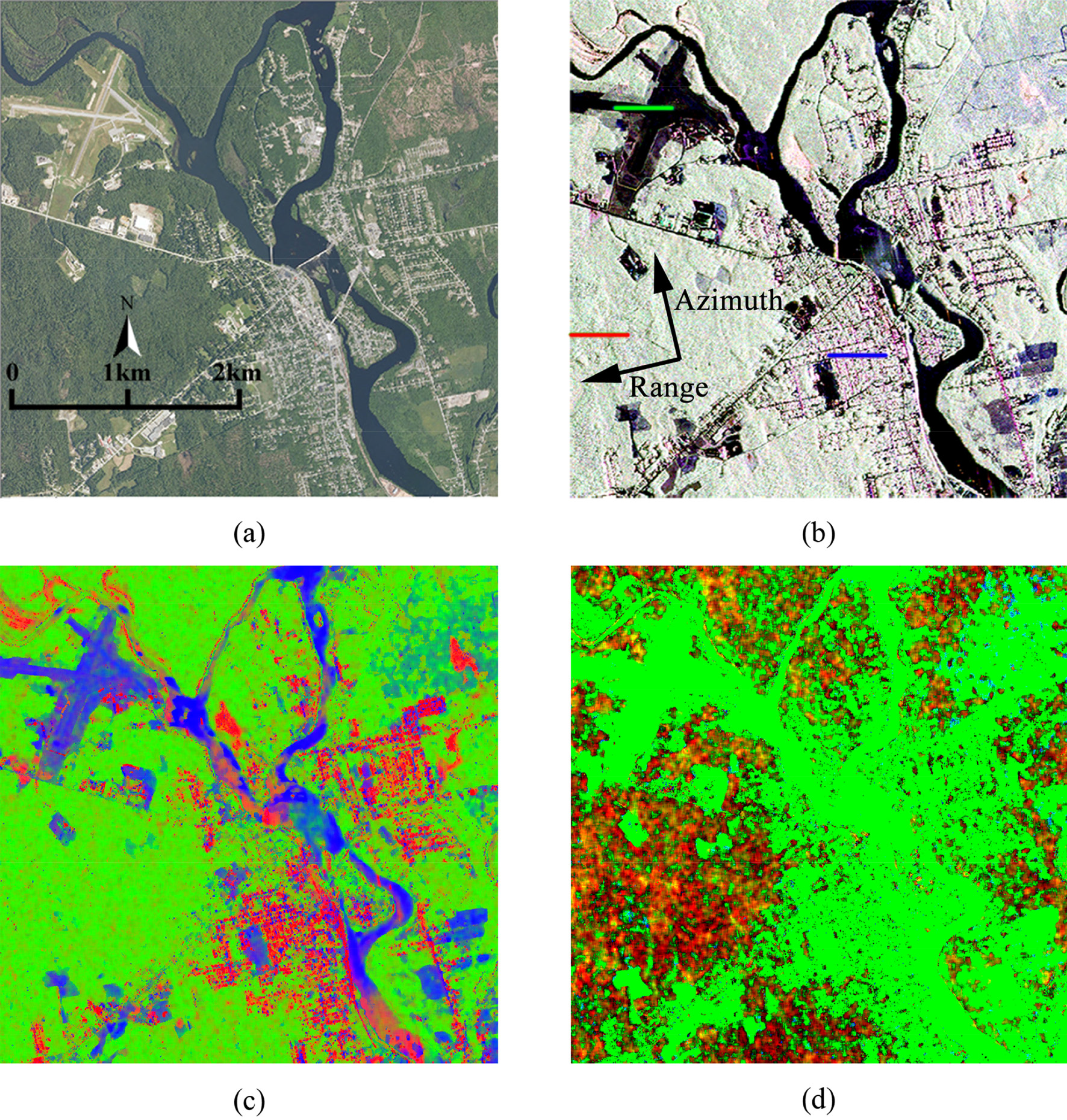
40]. UAVSAR data collected near Howland Forest, Maine, USA, on 5 August 2009 under a clear weather was used to test the applicability of proposed method. The study site is relatively flat and consists of forests, bare land, rivers, wetlands, road, buildings, etc. The data was downloaded from Alaska Satellite Facility website [41]. The look angle range is approximately [25°, 65°], while the local incidence angles vary within [0°, 90°]. Basic scattering area correction, antenna pattern correction and range dependent radiometric correction have been performed. The resolution of the ground range image is 5 m. Lee sigma filtering [42] is implemented in a 9 × 9 window. The equivalent number of looks is hard to estimate for ground range image because of lack of single look data. However, in multi-look slant range image, ensemble averaging was implemented with 12 looks in azimuth direction and three looks in range direction.
Among all pixels, 99.83% are perfectly fitted and only 0.17% cannot get good fitting of T12. Figure 3c is the image of component power normalized by Pspan, where Pspan is the span of 〈[T]〉. Figure 3d is the image of τ of different components.
From Figure 3c, we could see all the major land cover features are identified. Dense natural forests are colored with bright green, indicating PV is large. A large proportion of dense natural forests are characterized by non-zero PD and zero PS, although not all. τV mostly concentrates in [0.60, 0.90]. Non-zero τD primarily locates in dense natural forests with value in [0.03, 0.35]. Only a small number of forest pixels show non-zero τS. It is found that they mainly lie in the boundaries between forests and land with little vegetation cover. However, in forests with low canopy density, the pixels may have τS = 0 and τD = 0. In the upper right corner of the image, there exists a sparse forest. This area gets much higher proportion of PS compared with dense forests. Since the tree cover is low, it is reasonable to have more surface scattering from ground. In most locations of this sparse forest, τV = 1, τS = 0, and τD = 0, meaning volume scattering and helix scattering do explain all cross-polarized power. We could observe from Figure 3d that, generally, in forest, the easier to be accessed by human beings or the lower canopy density, the more likely to have τD = 0. We may interpret this phenomenon in the following way: in easily accessible forests, the terrain may be relatively flat and the understory may probably be underdeveloped; in the untraversed forests, the understory is fully developed, making the scattering process very complex. Most of the areas dominated by surface scattering, like river surfaces, airport, and grasslands, are colored with blue, showing that PS is quite high. In these areas, PS and PD are obtained with van Zyl’s method, thus, τS = 0 and τD = 0. In urban areas, the main buildings are oriented parallel to SAR azimuth direction. Many pixels near buildings are characterized by high PD while a small proportion show high PS. An apparent characteristic of these areas dominated by surface scattering or double bounce scattering is, they almost all have τV = 1, τS = 0, and τD = 0, which differs greatly from the dense natural forests.
The results of the proposed decomposition were compared with these of van Zyl decomposition and the other three latest NNED raised by Cui et al. [12] and Wang et al. [13]. Two NNED were raised by Cui et al. [
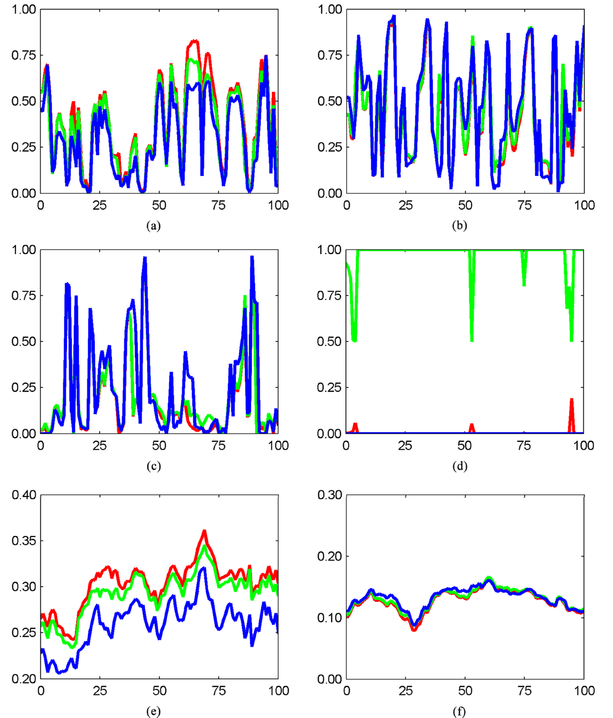
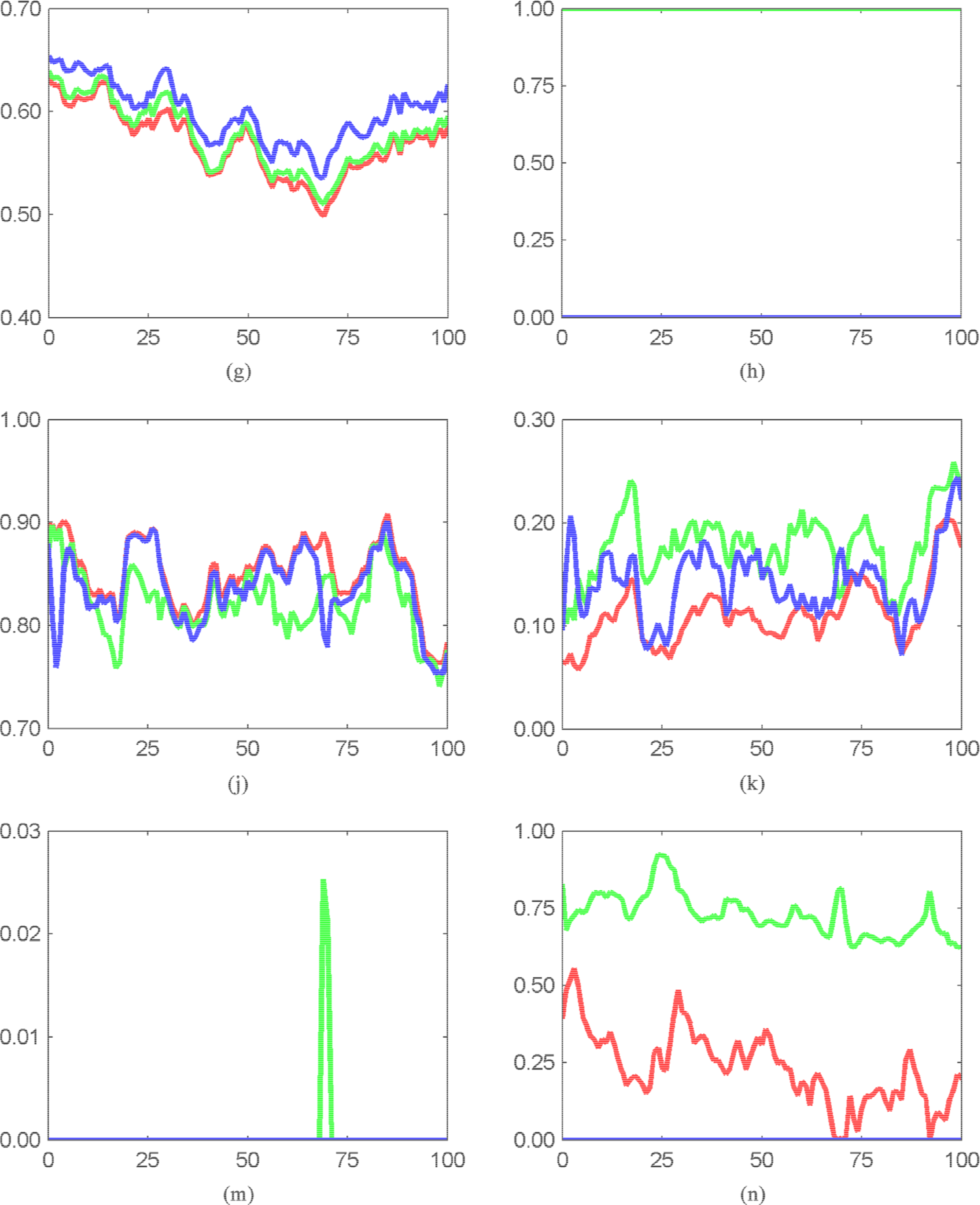
12] and they only differ in the decomposition of the remainder matrix, one is based on Eigen-decomposition, namely, Cui1, and the other on model fitting, namely, Cui2. It is found that the performance of Cui1 is not as good as Cui2 and Wang decomposition, while the results of Cui2 and Wang decomposition are quite similar. To avoid five profiles existing in one plot so the readers are confused, Figure 4 only gives the profiles of Wang, van Zyl and the proposed decomposition along three 500-m-long lines in Figure 3b. Red, green, and blue lines cover natural forests, airport, and urban areas, respectively.
Compared with van Zyl decomposition with OAC, the proposed decomposition lowered the estimation of PV in all pixels. The degree is −7.72% on average and the standard deviation is 0.103. In airports and almost all building areas, the proposed method gives the lowest estimation of PV. In locations 63 to 68 of Figure 4a, PV/Pspan is reduced by over 0.10. Consequently, at most locations, the PS + PD by the proposed decomposition are generally higher or at least equal to that by other decompositions. Several isolated pixels have positive τD, which may correspond to the trees in urban areas. In airport, PV/Pspan is lowered by more than 0.03, so we could observe the evident elevation of PS. PD by all three decompositions are approximately the same.
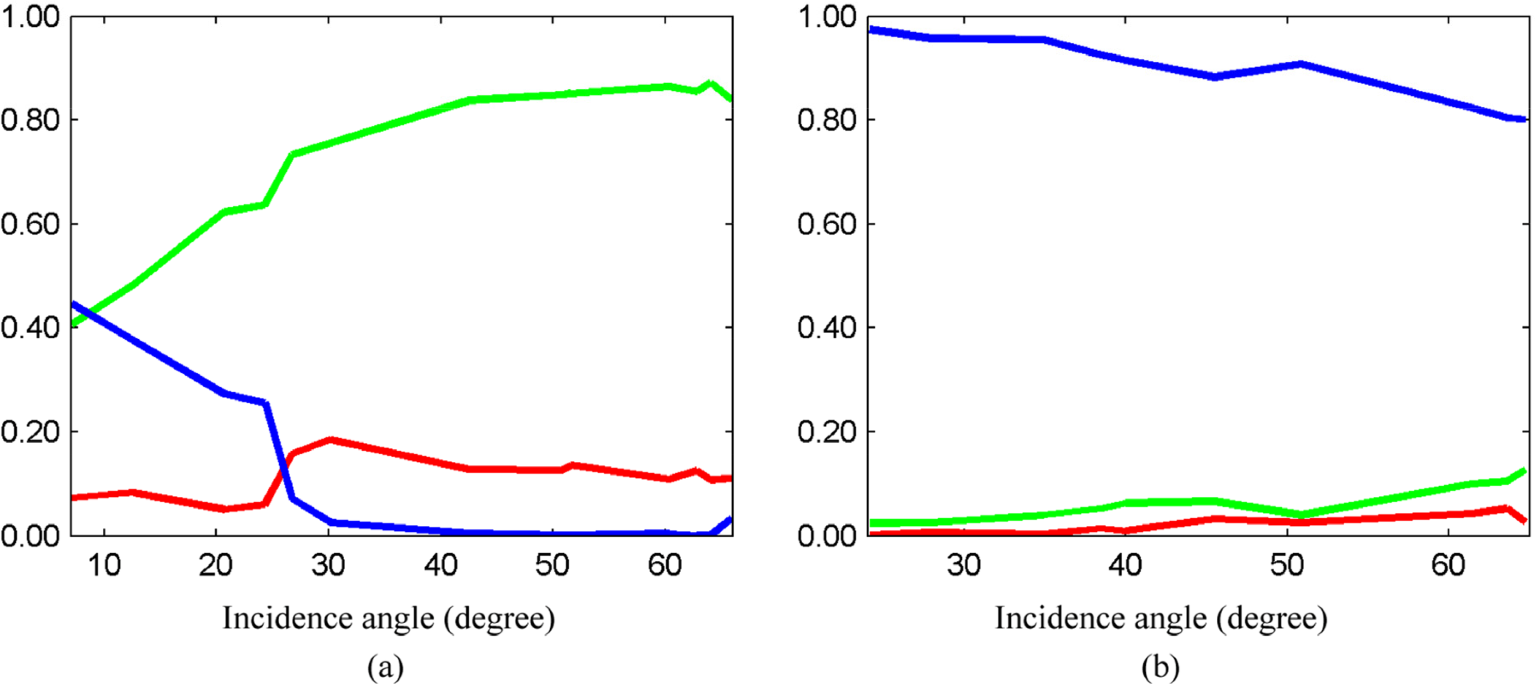
The dependency of decomposition results upon local incidence angles (short for incidence angle) was partly investigated. It is well known that SAR backscatter is influenced by land cover types and local incidence angle. Many land cover types reside in this study area, but it is difficult to select pixels with exactly the same land cover but different incidence angles. For simplicity, the authors just did this investigation for dense natural forests and lakes. First, dense natural forest and lake samples with the size 41 × 41 were selected in PolSAR image with the assistance of optical images. These samples could be roughly thought to be homogeneous inside. Next, the mean values of span-normalized powers of different components in diverse samples were plotted against their incidence angles (see Figure 5).
From Figure 5a, it seems the perspective that volume scattering dominates in dense natural forests only holds when the incidence angle is larger than a value, for example, 18°. When the incidence angle is medium or large, PV/Pspan can be over 0.75 and double-bounce is much stronger than surface scattering. However, if the incidence angle is smaller than a value, like 26°, with the decreasing of incidence angle, PV/Pspan drops quickly, at the same time, PS/Pspan goes up fast and surpasses PD/Pspan. If the incidence angle is smaller than 10°, PS/Pspan could be even larger than PV/Pspan.
To understand above facts, the authors treat the volume scattering caused by canopies to be approximately isotropic [43], thus, when other factors are fixed, the volume scattering power does not vary much when incidence angle changes. However, the ordinary ground or soil is not isotropic. The smaller incidence angles the stronger surface scattering power; the larger incidence angles the weaker surface scattering power. In forest, double-bounce scattering is usually caused by ground-trunk structure. When the incidence angle is large, although the first scattering occurring at ground is not so strong, the microwave backscattered by the tree bark could be relatively strong due to the smooth bark and small incidence angle of the second scattering. On the contrary, when the incidence angle is small, the second scattering occurring at bark has very large incidence angle, possibly making the backscattered microwave be weak in comparison to surface scattering. Here, we summarize that, with the decreasing of incidence angle, PS, Pspan, and PS/Pspan gradually increases; PV/Pspan drops which is mainly due to the increasing of Pspan.
Evidently, lakes are dominated by surface scattering, which is supported by the decomposition results in Figure 5b. No matter the incidence angle is small or large, PS/Pspan is always much larger than PD/Pspan and PV/Pspan. A basic trend is the larger incidence angle the smaller PS/Pspan.
Cheng [38] simulated PolSAR data with Bragg scatterer and incoherent scattering models. He observed such trend for surface scattering-dominated samples. He also found that the larger incidence angle the larger T33/Pspan. Since in most lake pixels, volume scattering and helix scattering explain all cross-polarized power, and τV = 1, we could easily infer that PV/Pspan increases with T33/Pspan or incidence angle.

5. Discussion

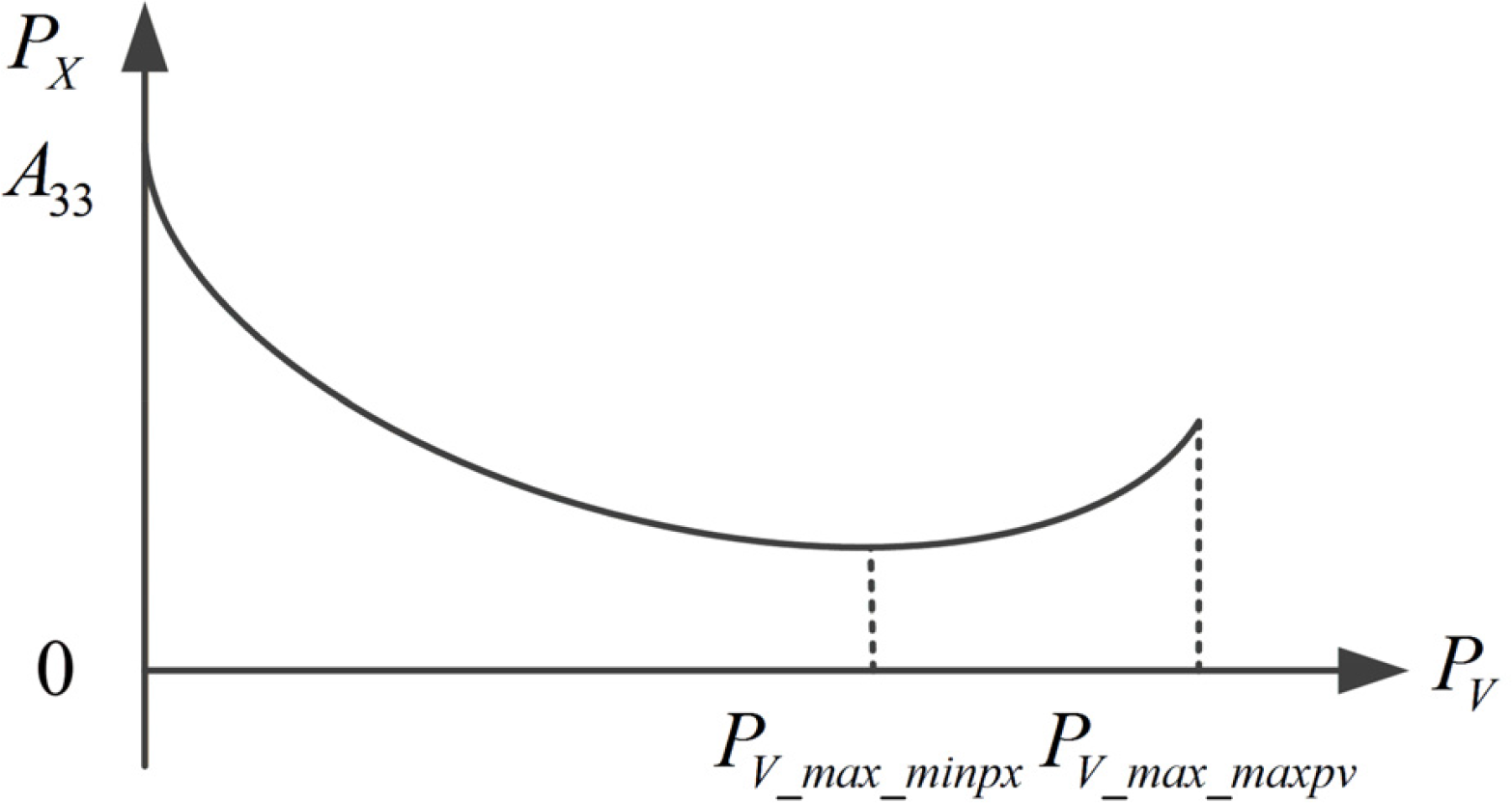
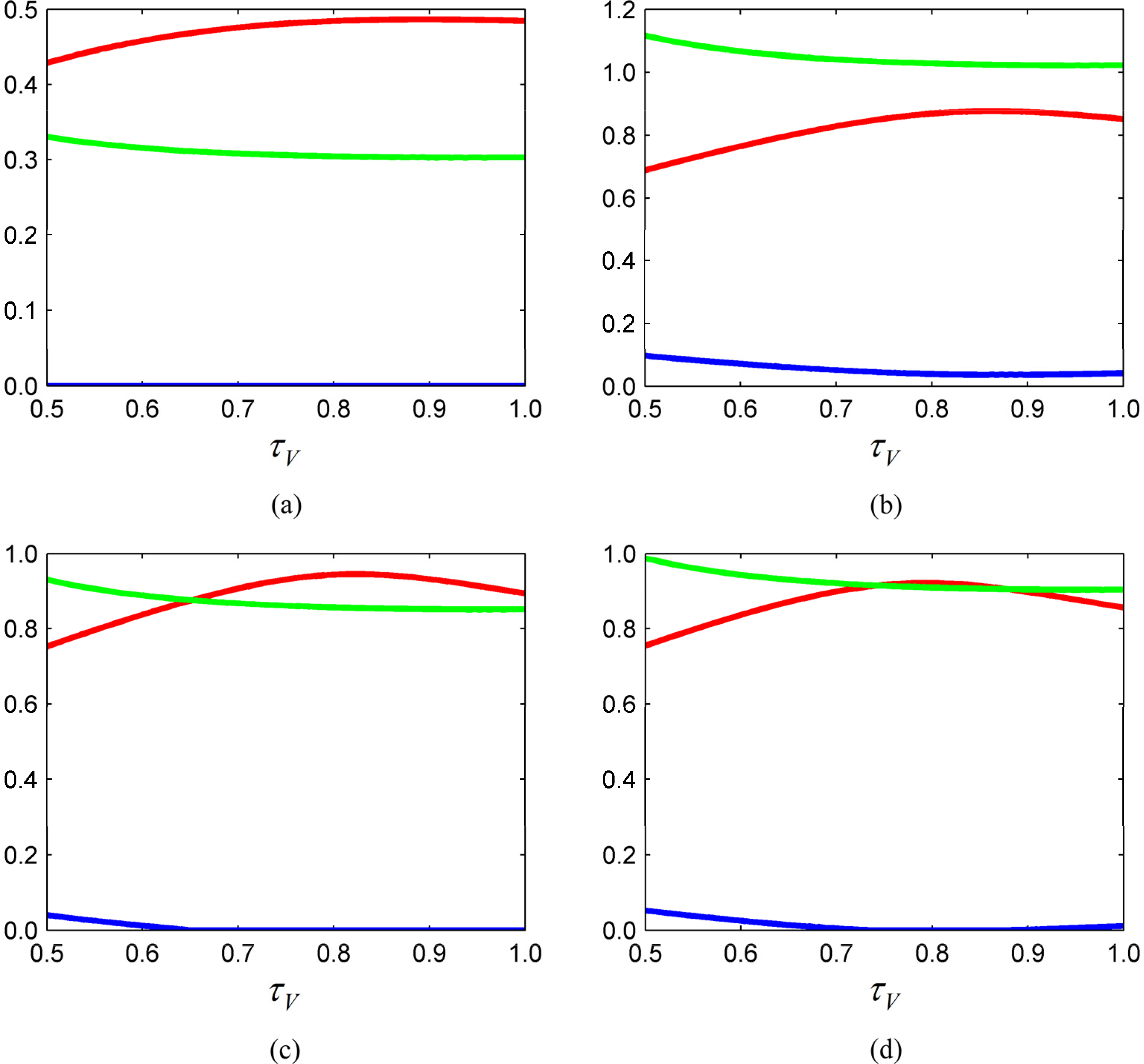
Experiment revealed the dependence of the decomposition results on land covers. Analytically explaining why these results are like this is challenging because many parameters are involved, so the authors show the relationship between τV and P0, P1, PX for four pixels, one is in airport and the other three are in forest (see Figure 6). Please note that if PV_max = P1, then PX = 0; if PV_max = P0, then PX > 0
From the sub-figures in Figure 6, we could know P1 is a monotonous decreasing function of τV. The relationship between P0 and τV is more complex: P0 first monotonously increases with τV until reaches a peak at τV = τV_0, then monotonously decreases with τV.
The line of P0 and the line of P1 are possible to have zero (see Figure 6a,b), one (see Figure 6c) or two (see Figure 6d) cross points. When these two lines do not intersect, then the situations are simple. It is observed that land covers dominated by surface scattering and double-bounce often have A33/Psp < 0.15, or even A33/Psp < 0.10, where Psp is the span of [TOAC_noh]. For the same τV, P1 is always smaller than P0 (see Figure 6a), then PV_max = P1. Finally, τV_maxpv = 0.5 < τV_minpx = 1.0, PV_max_maxpv.= 4A33/(1 − g(0.5)) > PV_max_minpx = 4A33· But as observed in UAVSAR data, dense natural forests usually show A33/Psp > 0.20. If A33/Pspan > 0.25, then P1 ≥ 4A33 > Psp, so the P1 line and P0 line never intersect, PV_max = P0 (see Figure 6b). In this case, τV_maxpv = τV_0 < τV_minpx, PV_max_maxpv > PV_max_minpx· Please remember that the P0 line and P1 line may do not intersect even when A33/Psp ≤ 0.25. Some forest pixels have P0 line and P1 line intersected with one or two cross points. When there is one cross point (see Figure 6c), assume the cross point is (τV_1, PV_max_1), then in [0.50, τV_1], PV_max = P0; in [τV_1, 1.0], PV_max = P Finally, τV_maxpv = τV_1 < τV_minpx = 1.0, PV_max_maxpv = PV_max_1 > PV_max_minpx = 4A33· When there are two cross points, assume the two cross points are (τV_1, PV_max_1) and τV_2, PV_max_2), and τV_2 > τV_1, then in [0.50, τV_1] and [τV_2, 1.0], PV_max = P0; in [τV_1, τV_2], PV_max = P Finally, τV_maxpv = τV_1 < τV_minpx = τV_2, PV_max_maxpv = PV_max_1 > PV_max_minpx = PV_max_
Why PV by the proposed decomposition is lower than that by van Zyl decomposition has been proven in previous sections. When it comes to the comparison between the proposed method and Wang decomposition, quantitatively explaining is much more difficult because Wang decomposition computes volume scattering parameters without RSA which is equal to solving cubic equations. Cheng [38] proved that for a fixed [TV], PV computed without RSA is usually smaller than that computed with RSA. As a result, we are not sure whether PV computed without RSA and with maximum PV criterion is larger, or PV computed with RSA and minimum PV criterion is larger. That explains the situations of forest. For pixels dominated by surface scattering and double-bounce scattering, Wang decomposition commonly gives τV = 0.5, on the contrary, the proposed method has τV = 1.0. According to Equation (21), to explain the same amount of cross-polarized power, PV by Wang decomposition needs to be larger than that by the proposed method.
With simulated data, Cheng [38] found the proposed decomposition works worst in areas dominated by double-bounce scattering. In surface scattering-dominated areas, the cross-polarized power is usually relatively low, so even if we think cross-polarized power is entirely from volume scattering, the given PV will not be large. For areas dominated by volume scattering, letting volume scattering explain the most cross-polarized power in theory is reasonable to a large degree. However, it was pointed out in [36,37] that T33 of double-bounce scattering model may be comparable to that of volume scattering model. In other words, sometimes, double-bounce scattering produces significant cross-polarized power. Minimum PX criterion forces volume scattering to explain as much cross-polarized power as possible. Therefore, a proportion of explained cross-polarized power is probably from double-bounce scattering instead of volume scattering. In this sense, PV may be overestimated.

6. Conclusions

The main differences between the proposed method and van Zyl, Cui, Wang’s NNED include: (1) helix scattering are introduced in our method; (2) our method use minimum PX criterion while the three NNED use maximum PV criterion; (3) sometimes the dominant ground scattering is described by incoherent and depolarizing models, so there is no remainder component. In the three NNED, ground scattering are all coherently modeled; (4) to describe ground scattering, Cui and Wang NNED use elemental scatterers with SHV ≠ 0, but our method utilizes elemental scatterers with SHV = 0.
Negative component power is completely avoided in the proposed decomposition. In the experiment done by Cheng [38] with simulated data, he found that compared with van Zyl decomposition, the proposed method is capable of partly lessening volume scattering overestimation, which is mainly achieved by introducing helix scattering, utilizing minimum PX criterion, and performing two-component fitting to [TOAC_noh]. But Cheng [38] also emphasized that minimum PX criterion could not fully eliminate PV overestimation in that volume scattering probably cannot explain the most cross-polarized power in theory. Ground scattering also contributes to cross-polarized power. The proposed method usually better estimates the power of each component than van Zyl, Wang and Cui decomposition. One significant advantage of the proposed method is, when volume scattering and helix scattering cannot explain all cross-polarized power, the dominant ground scattering is modeled by depolarizing models, so that its orientation angle randomness could be obtained. In the proposed decomposition, all cross-polarized power is explained by models with solid physical meanings.
How to utilize the power, complex scattering coefficients, orientation angle randomness of different components given by the proposed method for the applications like land cover mapping, scattering mechanism classification, understory mapping, or surface roughness and soil moisture estimation, needs more research. Another future research direction is proposing a decomposition that computes volume scattering parameters without RSA to utilize T13 in [TOAC_noh].

Acknowledgments

This work was supported by the National Key Fundamental Research Plan of China (973) under Grant 2012CB719906. The authors would like to thank UAVSAR team in Jet Propulsion Laboratory, NASA for processing and providing UAVSAR data and the reviewers for reviewing this paper.

Author Contributions

Xiaoguang Cheng is the main proposer of the method in this paper as well as the chief author of this paper. Wenli Huang made great contribution to the improvement of language and writing of this paper. Jianya Gong provided much guidance to Xiaoguang Cheng in experiment design.

Conflicts of Interest

The authors declare no conflict of interest.

References

  1. Ouchi, K. Recent trend and advance of synthetic aperture radar with selected topics. Remote Sens 2013, 5, 716–807. [Google Scholar]
  2. Freeman, A.; Durden, S.L. A three-component scattering model to describe polarimetric SAR data. Proc. SPIE 1992, 1748, 213–225. [Google Scholar]
  3. Freeman, A.; Durden, S.L. A three-component scattering model for polarimetric SAR data. IEEE Trans. Geosci. Remote Sens 1998, 36, 963–973. [Google Scholar]
  4. Yamaguchi, Y.; Moriyama, T.; Ishido, M.; Yamada, H. Four-component scattering model for polarimetric SAR image decomposition. IEEE Trans. Geosci. Remote Sens 2005, 43, 1699–1706. [Google Scholar]
  5. An, W.; Cui, Y.; Yang, J. Three-component model-based decomposition for polarimetric SAR data. IEEE Trans. Geosci. Remote Sens 2010, 48, 2732–2739. [Google Scholar]
  6. Arii, M.; van Zyl, J.J.; Kim, Y. Adaptive model-based decomposition of polarimetric SAR covariance matrices. IEEE Trans. Geosci. Remote Sens 2011, 49, 1104–1113. [Google Scholar]
  7. Van Zyl, J.J.; Arii, M.; Kim, Y. Model-based decomposition of polarimetric SAR covariance matrices constrained for nonnegative eigenvalues. IEEE Trans. Geosci. Remote Sens 2011, 49, 3452–3459. [Google Scholar]
  8. Cui, Y.; Yamaguchi, Y.; Yang, J.; Park, S.-E.; Kobayashi, H.; Singh, G. Three-component power decomposition for polarimetric SAR data based on adaptive volume scatter modeling. Remote Sens 2012, 4, 1559–1572. [Google Scholar]
  9. Singh, G.; Yamaguchi, Y.; Park, S.E. General four-component scattering power decomposition with unitary transformation of coherency matrix. IEEE Trans. Geosci. Remote Sens 2013, 51, 3014–3022. [Google Scholar]
  10. Singh, G.; Yamaguchi, Y.; Park, S.E.; Cui, Y.; Kobayashi, H. Hybrid freeman/eigenvalue decomposition method with extended volume scattering model. IEEE Geosci. Remote Sens. Lett 2013, 10, 81–85. [Google Scholar]
  11. Chen, S.-W.; Wang, X.-S.; Xiao, S.-P.; Sato, M. General polarimetric model-based decomposition for coherency matrix. IEEE Trans. Geosci. Remote Sens 2014, 52, 1843–1855. [Google Scholar]
  12. Cui, Y.; Yamaguchi, Y.; Yang, J.; Kobayashi, H.; Park, S.E.; Singh, G. On complete model-based decomposition of polarimetric SAR coherency matrix data. IEEE Trans. Geosci. Remote Sens 2014, 52, 1991–2001. [Google Scholar]
  13. Wang, C.; Yu, W.; Wang, R.; Deng, Y.; Zhao, F. Comparison of nonnegative eigenvalue decompositions with and without reflection symmetry assumptions. IEEE Trans. Geosci. Remote Sens 2014, 52, 2278–2287. [Google Scholar]
  14. Freeman, A. Fitting a two-component scattering model to polarimetric SAR data from forests. IEEE Trans. Geosci. Remote Sens 2007, 45, 2583–2592. [Google Scholar]
  15. Jong-Sen, L.; Ainsworth, T.L.; Yanting, W. Generalized polarimetric model-based decompositions using incoherent scattering models. IEEE Trans. Geosci. Remote Sens 2014, 52, 2474–2491. [Google Scholar]
  16. Antropov, O.; Rauste, Y.; Hame, T. Volume scattering modeling in POLSAR decompositions: Study of ALOS PALSAR data over boreal forest. IEEE Trans. Geosci. Remote Sens 2011, 49, 3838–3848. [Google Scholar]
  17. Da Silva, A.; Paradella, W.; Freitas, C.; Oliveira, C. Evaluation of digital classification of polarimetric SAR data for iron-mineralized laterites mapping in the amazon region. Remote Sens 2013, 5, 3101–3122. [Google Scholar]
  18. Lönnqvist, A.; Rauste, Y.; Molinier, M.; Häme, T. Polarimetric SAR data in land cover mapping in boreal zone. IEEE Trans. Geosci. Remote Sens 2010, 48, 3652–3662. [Google Scholar]
  19. Lardeux, C.; Frison, P.L.; Tison, C.; Souyris, J.C.; Stoll, B.; Fruneau, B.; Rudant, J.P. Support vector machine for multifrequency SAR polarimetric data classification. IEEE Trans. Geosci. Remote Sens 2009, 47, 4143–4152. [Google Scholar]
  20. Lee, J.-S.; Grunes, M.R.; Pottier, E.; Ferro-Famil, L. Unsupervised terrain classification preserving polarimetric scattering characteristics. IEEE Trans. Geosci. Remote Sens 2004, 42, 722–731. [Google Scholar]
  21. Qi, Z.; Yeh, A.G.-O.; Li, X.; Lin, Z. A novel algorithm for land use and land cover classification using RADARSAT-2 polarimetric SAR data. Remote Sens. Environ 2012, 118, 21–39. [Google Scholar]
  22. Lee, J.-S.; Grunes, M.R.; Schuler, D.L.; Pottier, E.; Ferro-Famil, L. Scattering-model-based speckle filtering of polarimetric SAR data. IEEE Trans. Geosci. Remote Sens 2006, 44, 176–187. [Google Scholar]
  23. Ballester-Berman, J.D.; Lopez-Sanchez, J.M. Applying the freeman-durden decomposition concept to polarimetric SAR interferometry. IEEE Trans. Geosci. Remote Sens 2010, 48, 466–479. [Google Scholar]
  24. Yajima, Y.; Yamaguchi, Y.; Sato, R.; Yamada, H.; Boerner, W.-M. Polsar image analysis of wetlands using a modified four-component scattering power decomposition. IEEE Trans. Geosci. Remote Sens 2008, 46, 1667–1673. [Google Scholar]
  25. Shi, J.; Lee, J.-S.; Chen, K.; Sun, Q. Evaluate usage of decomposition technique in estimation of soil moisture with vegetated surface by multi-temporal measurements. Proceedings of the 2000 IEEE International Geoscience and Remote Sensing Symposium, Honolulu, HI, USA, 25–30 July 2000; 3, pp. 1098–1100.
  26. Hajnsek, I.; Jagdhuber, T.; Schön, H.; Papathanassiou, K.P. Potential of estimating soil moisture under vegetation cover by means of POLSAR. IEEE Trans. Geosci. Remote Sens 2009, 47, 442–454. [Google Scholar]
  27. Jagdhuber, T.; Schön, H.; Hajnsek, I.; Papathanassiou, K.P. Soil moisture estimation under vegetation applying polarimetric decomposition techniques. In Proceedings of the 4th International Workshop on Science and Applications of SAR Polarimetry and Polarimetric Interferometry, Frascati, Italy, 26–30 January 2009; ESA: Frascati, Italy, 2009. pp. 1–8.
  28. Tello, M.; López-Martínez, C.; Mallorqui, J.J. A novel algorithm for ship detection in SAR imagery based on the wavelet transform. IEEE Geosci. Remote Sens. Lett 2005, 2, 201–205. [Google Scholar]
  29. Sato, R.; Takahashi, Y.; Yamaguchi, Y.; Yamada, H. stricken man-made object detection using scattering power decomposition with NNED and rotation of the covariance matrix. In Proceedings of the 2012 IEEE International Geoscience and Remote Sensing Symposium, Munich, Germany, 22–27 July 2012; pp. 5121–5124.
  30. Yonezawa, C.; Watanabe, M.; Saito, G. Polarimetric decomposition analysis of ALOS PALSAR observation data before and after a landslide event. Remote Sens 2012, 4, 2314–2328. [Google Scholar]
  31. Arii, M.; van Zyl, J.J.; Kim, Y. A general characterization for polarimetric scattering from vegetation canopies. IEEE Trans. Geosci. Remote Sens 2010, 48, 3349–3357. [Google Scholar]
  32. Neumann, M. Remote Sensing of Vegetation Using Multi-Baseline Polarimetric Sar Interferometry: Theoretical Modeling and Physical Parameter Retrieval.
  33. Lee, J.-S.; Ainsworth, T.L. The effect of orientation angle compensation on coherency matrix and polarimetric target decompositions. IEEE Trans. Geosci. Remote Sens 2011, 49, 53–64. [Google Scholar]
  34. Chen, S.-W.; Ohki, M.; Shimada, M.; Sato, M. Deorientation effect investigation for model-based decomposition over oriented built-up areas. IEEE Geosci. Remote Sens. Lett 2013, 10, 273–277. [Google Scholar]
  35. Neumann, M.; Ferro-Famil, L.; Pottier, E. A. General model based polarimetric decomposition scheme for vegetated areas. Proceedings of the 4th International Workshop on Science and Applications of SAR Polarimetry and Polarimetric Interferometry (ESRIN), Frascati, Italy, 26–30 January 2009.
  36. Cheng, X.; Huang, W.; Gong, J. An unsupervised scattering mechanism classification method for polsar images. IEEE Geosci. Remote Sens. Lett 2014, 11, 1677–1681. [Google Scholar]
  37. Cheng, X.; Huang, W.; Gong, J. A decomposition-free scattering mechanism classification method for PoLSAR images with Neumann’s model. Remote Sens. Lett 2013, 4, 1176–1184. [Google Scholar]
  38. Cheng, X. Research of Model-Based Polarimetric Sar Decomposition Constrained for Nonnegative Eigenvalues.
  39. Rosen, P.A.; Hensley, S.; Wheeler, K.; Sadowy, G.; Miller, T.; Shaffer, S.; Muellerschoen, R.; Jones, C.; Zebker, H.; Madsen, S. UAVSAR: A new NASA Airborne SAR system for science and technology research. Proceedings of the 2006 IEEE Conference on Radar, Verona, NY, USA, 24–27 April 2006; pp. 22–29.
  40. UAVSAR-Home. Available online: http://uavsar.jpl.nasa.gov/instrument.html (accessed on 4 September 2013).
  41. Vertex: ASF’s Data Portal. Available online: https://vertex.daac.asf.alaska.edu (accessed on 1 May 2012).
  42. Lee, J.-S.; Wen, J.-H.; Ainsworth, T.L.; Chen, K.-S.; Chen, A.J. Improved sigma filter for speckle filtering of SAR imagery. IEEE Trans. Geosci. Remote Sens 2009, 47, 202–213. [Google Scholar]
  43. Cheng, X.; Pinto, N.; Gong, J. Terrain radiometric calibration of airborne UAVSAR for forested area. Geo-Spat. Inf. Sci 2012, 15, 229–240. [Google Scholar]

Appendix

To simplify the computation of SHH and SVV, we assume SHH = 1 and SVV = b1 + b2j as that in Freeman-Durden decomposition [3]. Take them into [TRemainder2], if Im(G12) ≠ 0, we have
L N = ( 1 + b 1 ) 2 + b 2 2 ( 1 b 1 ) 2 + b 2 2 = G 1 G 22 + G 33 = k 1
Re ( M ) Im ( M ) = 1 b 1 2 b 2 2 2 b 2 = Re ( G 12 ) Im ( G 12 ) = k 2
The solutions of (A1) and (A2) are
b 1 = ( k 1 1 ) ( ( 1 + k 2 2 ) ( 1 + k 1 ) k 2 σ ) D 2 k 1 b 2 = σ k 1 ( 4 k 2 + σ ) D
and
b 1 = ( k 1 1 ) ( ( 1 + k 2 2 ) ( 1 + k 1 ) + k 2 σ ) D 2 k 1 b 2 = σ + k 1 ( 4 k 2 + σ ) D
with
σ = 2 k 1 ( k 2 2 + 1 )
D = ( k 1 2 + 1 ) ( k 2 2 + 1 ) 2 k 1 ( k 2 2 1 )
For the two solutions in Equations (A3) and (A4), the one whose b2 sign is the same as Im(G12) should be chosen. If Im(G12) = 0, then b2 = 0, b1 is
b 1 = k 1 1 k 1 + 1
or
b 1 = k 1 + 1 k 1 1
The two b1 solutions in Equations (A7) and (A8) are the inverse of each other. Which one is better may be determined with the help of physical models, like Bragg model [26]. For example, for surface scattering, Bragg model predicts |SVV| < 1, so the smaller one of Equations (A7) and (A8) should be chosen.
Figure 1. The flow chart of the proposed decomposition.
Remotesensing 06 06365f1
Figure 2. The difference between minimum PX criterion and maximum PV criterion.
Remotesensing 06 06365f2
Figure 3. (a) Optical images from National Agriculture Imagery Program (short for NAIP and administered by USDA-FSA Aerial Photography Field Office) 2009; (b) Pauli color-coded image; (c) Image composed of different components power, red is for PD/Pspan, green is for PV/Pspan, and blue is for PS/Pspan; (d) Image composed of τ of different components, red is for τD, green is for τV, and blue is for τS. The geographic coordinate of image center is 68.656°W, 44.943°N.
Remotesensing 06 06365f3
Figure 4. Horizontal axis is pixel’s relative position along profile. (ad) are the profiles along the blue lines in Figure 3b; (eh) are the profiles along the green lines in Figure 3b; (jn) are the profiles along the red lines in Figure 3b; (a,e,j) are the profiles of PV/Pspan; (b,f,k) are PD/Pspan; (c,g,m) are PS/Pspan. In above 9 subfigures, red lines are the results of van Zyl decomposition, green lines are the results of Wang, and blue lines are the results of the proposed method; (d,h,n) are the τ profiles along the blue, green, and red lines in Figure 3b, respectively. In (d,h,n), red line is τD, green line is τV, blue line is τS.
Remotesensing 06 06365f4aRemotesensing 06 06365f4b
Figure 5. The relationship between normalized component powers and incidence angles. (a) Dense natural forest data; (b) Lake data. In both sub-figures, red line stands for PD/Pspan, green line stands for PV/Pspan, and blue line stands for PS/Pspan.
Remotesensing 06 06365f5
Figure 6. The relationship between τV and P0, P1, PX· (a) A pixel in airport; (bd) are pixels in forest. In all sub-figures, red line stands for P0/Psp, green line stands for P1/Psp, and blue line stands for PX/Psp, where Psp is the span of [TOAC_noh].
Remotesensing 06 06365f6

