Improving Lithological Mapping by SVM Classification of Spectral and Morphological Features: The Discovery of a New Chromite Body in the Mawat Ophiolite Complex (Kurdistan, NE Iraq)


Abstract
: The mineral ore potential of many mountainous regions of the world, like the Kurdistan region of Iraq, remains unexplored. For logistical and sometimes political reasons, these areas are difficult to map using traditional methods. We highlight the improvement in remote sensing geological mapping that arises from the integration of geomorphic features in classifications. The Mawat Ophiolite Complex (MOC) is located in the NE of Iraq and is known for its mineral deposits. The aims of this study are: (I) to refine the existing lithological map of the MOC; (II) to identify the best discriminatory datasets for lithological classification, including geomorphic features and textures; and (III) to identify potential locations with high concentrations of chromite. We performed a Support Vector Machine (SVM) classification method to allow the joint use of geomorphic features, textures and multispectral data of the Advanced Space-borne Thermal Emission and Reflection radiometer (ASTER) satellite. The updated map allowed the identification of a new mafic body and a substantial improvement of the geometry of the known lithological units. The use of geomorphic features allowed for the increase of the overall accuracy from 73% to 79.3%. In addition, we detected chromite occurrences within the ophiolite by applying Spectral Angle Mapping (SAM) technique. We identified two new locations having high concentrations of chromite and verified one of these promising areas in the field. This new body covers ∼0.3 km2 and has coarsely crystalline chromite within dunite host rock. The chromium (Cr2O3) concentration is ∼8.46%. The SAM and SVM methods applied on ASTER satellite data show that these can be used as a powerful tool to explore ore deposits and to further improve lithological mapping in mountainous semi-arid regions.1. Introduction
Geological maps provide basic information that can be used in a variety of domains such as tectonics, landslide hazard assessment, engineering projects, exploration of groundwater, petroleum and mineral resources studies [1]. Geological mapping and mineral exploration mainly relies on fieldwork and more recently, on remote sensing studies. Conducting field surveys in complex and poorly accessible terrain is challenging, expensive and time-consuming. In contrast, remote sensing data can provide detailed information over large areas, especially in arid and semi-arid regions. It is cost effective and efficient, particularly in remote areas where collecting field observations is difficult [2,3].
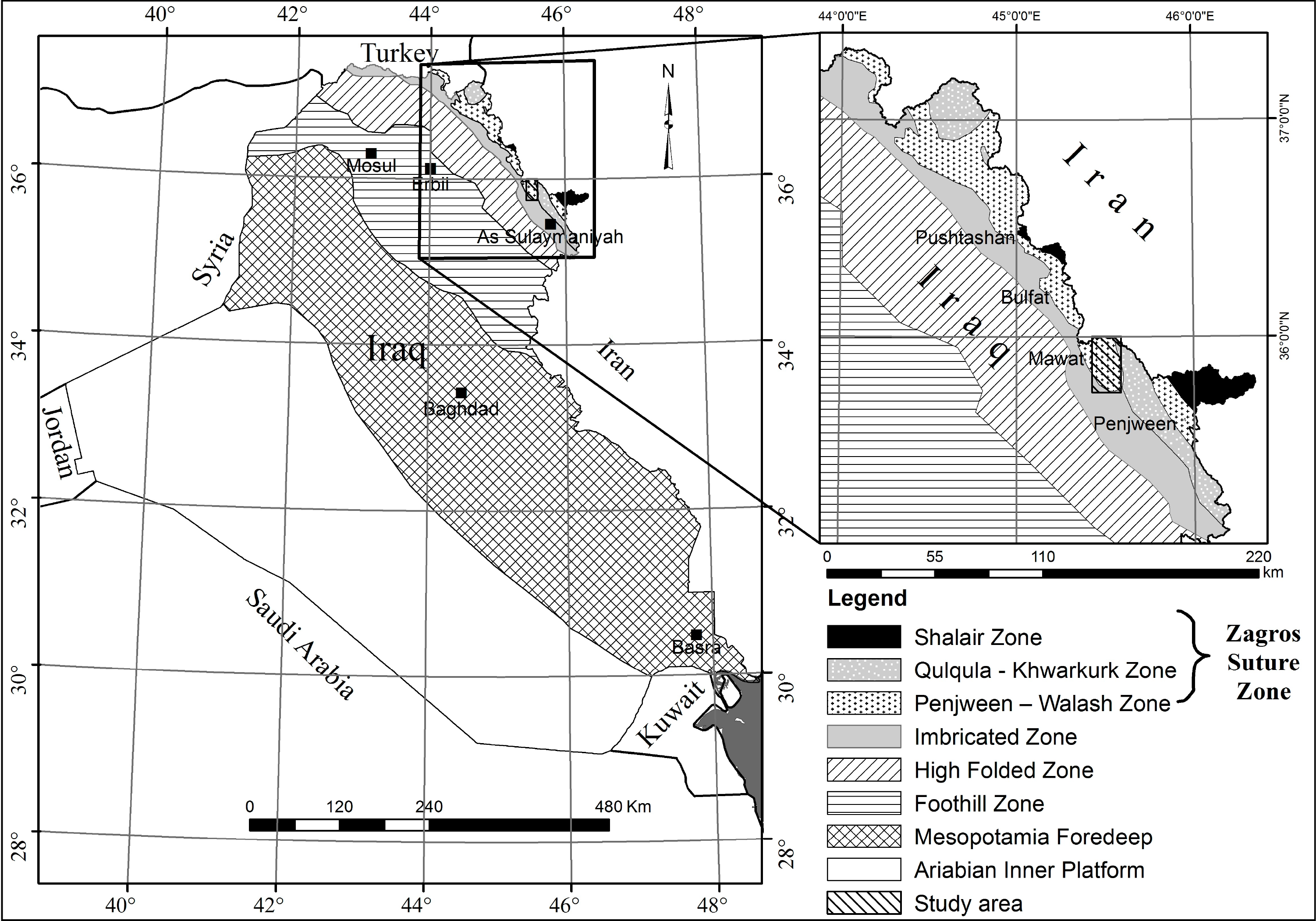
The Zagros orogenic belt formed by the collision between the Arabian and the Eurasian margins, and the closure of the Neo-Tethys [4–6]. The shortening of the Zagros orogenic belt resulted from the ongoing subduction of the Arabian plate beneath the Eurasian plate [4–6]. The occurrence of ophiolite complexes corresponds to the suture between those plates [4–6]. The sequence of a classic “Penrose type” ophiolite from bottom to top is ultramafic complex, gabbroic complex, mafic volcanic complex and associated rocks such as overlying sedimentary rocks [7–10]. The Iraqi part of the Zagros Suture Zone in N and NE Iraq contains four complexes of Cretaceous Mawat, Cretaceous Penjween, Cretaceous Pushtashan, and Palaeogene Bulfat (Figure 1, [6,9,11]). The Mawat Ophiolite Complex (MOC) displays a complete ophiolite sequence, while the other three complexes are incomplete [9].
Spectral remote sensing data have been widely used to geological mapping and mineral exploration [2,12–21], particularly in high outcrop density areas. Remote sensing data have been applied to map ophiolite complexes in the Zagros suture zone of the Iranian section, e.g., [22–24]; however, these complexes have not yet been studied by remote sensing in the Zagros suture zone of the Iraqi section. Nevertheless, many field surveys were applied in the MOC. The first geological map of the MOC at a scale of 1:100,000 was compiled by Bolton et al. [25]. Later, in 1954, Bolton [26] modified six geological maps at scale of 1:100,000 covering the MOC [25]. Smirnov and Nelidov [27] classified the Mawat as an intrusion igneous complex. In 1974, Al-Mehaidi [28] reclassified The MOC as an ophiolite complex. The deficiencies in the previous geological map are related to the absence of quaternary sediments and the non-discrimination of the Walash and Naopurdan sequences as separate sedimentary and volcanic units [28]. Indeed, there is a mismatch between the geological maps of Iranian and Iraqi sides (Figure 2, [28–30]). The deficiency of those works [25–28] is one of the main reasons that motivate us to update the MOC lithological map. The other reason is that the MOC has not been studied thoroughly by remote sensing, while previous field survey studies revealed that the MOC is a promising area for chromite deposits [25–28].
The objectives of this study were threefold: (1) to update the former lithological map of the MOC using SVM technique to allow the joint use of spectral and DEM data; (2) To carry out a comparison of the data sets, which variously consider or ignore geomorphic features, and identify the best discriminatory set for lithological classification; (3) To identify potential areas hosting high concentrations of chromite in the MOC using Spectral Angle Mapping (SAM) technique.
In this research, we produced reflectance, at-sensor brightness temperatures, entropy and second moment textures features from ASTER and calculated geomorphic parameters from Digital Elevation Model (DEM) data. The most suitable geomorphic feature is the surface index (SI), a new and efficient index, which is able to map preserved and eroded portions of an elevated landscape at the same time [31,32]. Since we have many layers with different distributions, we used a Support Vector Machine (SVM) classification technique, as the SVM is suggested to be independent of complicated class distributions in multi- and hyperspectral data [33,34]. The accuracy of the lithological maps is evaluated by independent validation samples, fieldwork, and former lithological map. The potential areas hosting high concentrations of chromite were evaluated by laboratory analysis on collected samples from fieldwork.
2. Location and Geological Setting
The study area is located between 36°00′N and 35°45′N and between 45°26′E and 45°35′E. It comprises the Iraq Zagros Mountains and is characterized by rough topography with elevations from 661 m to 2360 m (a.s.l.). The slopes range between flat and 65°. Spread of anti-personnel mines (remnants from the Iran-Iraq war) over the study area makes it difficult to reach. The studied area covers about 422 km2, and encompasses part of the Sulaimaniyah Governorate/Kurdistan Region in NE Iraq, and small parts of the West Azerbaijan and Kordestan Provinces in Iran (Figure 1). The Mawat area is characterized by dry summers and wet winters. The entire annual precipitation (896 mm) occurs from October to May. The snowfalls occur for more than 10 days per year on average between November and April. Monthly temperatures ranges between −2.1 °C (January) and 37.3 °C (August). Wheat, barley, lentil, almond, walnut, pistachio, apricot, oak, pomegranate and grape are the dominant crops and fruits in the region.
The Zagros orogenic belt is part of the Alpine-Himalayan mountain ranges and trends in the NW-SE direction. This belt is around 2000 km long, extending from SE Turkey through Iraq to southern Iran [35–38]. The Iraqi part of the Zagros orogenic belt consists of three main tectonic zones: (1) the Inner Platform (stable shelf); (2) the Outer Platform (unstable shelf), which comprises the Mesopotamia Foredeep, the Foothill Zone, the High Folded Zone, and the Imbricated Zone (IZ); and (3) the Zagros Suture Zone (ZSZ) ([9,30,36,39,40]; Figure 1). Most of the study area lies within the ZSZ, represented by the Penjween-Walash Zone (PWZ), the Qulqula-Khwarkurk Zone (QKZ), and a small part of the Arabian Outer Platform (unstable shelf) represented by the IZ (Figure 1).
The study area consists of different lithostratigraphic sunits (Figure 2), which formed through the Late Cretaceous and Mio-Pliocene periods. The IZ includes three formations; two of them (Shiranish and Tanjero Formations) cover a small area, while the Aqra-Bekhme Formation covers a large area. These formations are composed mainly of limestones, calcareous sandstones, marls, mudstones, shales, and conglomerates [9,26,27,41,42]. The Red beds series include four lithostratigraphic units which comprise silty shales, conglomerates, sandstones, marls, limestones and were deposited during the Tertiary [9,27,42].
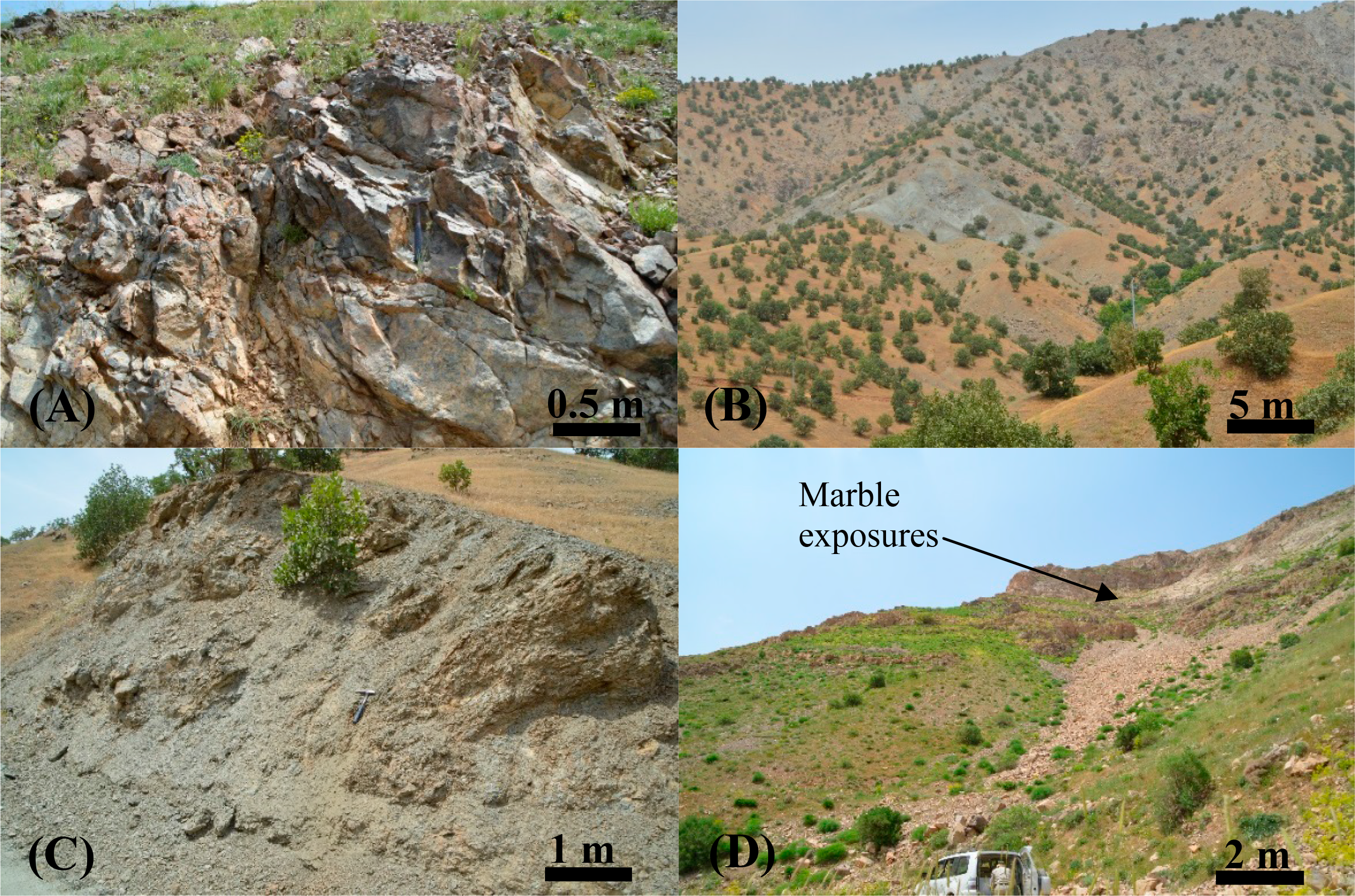
Three tectonic zones form the ZSZ of which only two (the PWZ and the QKZ) lie in the study area. The PWZ includes three tectonic units. (1) The MOC, which has been divided into three members (from bottom to top; Figure 2): the early Cretaceous-Cenomanian ultramafics, gabbro and metabasalt (Figure 3A–C); (2) The Gimo Calcareous Group, obducted during early Late Cretaceous over the metabasalt of the MOC. It is composed of massive marbles (Figure 3D) and calc-schists interbedded with basaltic flows; (3) The Walash and Naopurdan sequences of Paleocene-Oligocene age build a narrow band around the edge of the MOC. The QKZ located in the eastern part of the MOC, it is represented by the Qulqula radiolarian group of Aptian-Albian age. It consists of radiolarian mudstone, chert, limestone and pebbly conglomerate rocks. The Walash sequence comprises sedimentary shale, greywacke, limestones, volcanic basalt, andesite, tuffs, and agglomerates. The Naopurdan Sequence consists of silty shale, greywacke, sand, limestone, pebbly conglomerate, breccia, ashes and occasionally intruded by dykes [9,27,42]. Field observation shows that the Walash sequence involve serpentine bodies, which normally are rich in chromite. The Walash and Naopurdan sequences are located between the two main thrust faults and clearly mark the upper and lower contacts. The two thrusted sheets have steep slopes, folds of chevron type, and contain boudinage structures. The intrusions of serpentine rocks are associated with the thrust fault.
3. Methodology
3.1. Data Characteristics and Software
ASTER is a multi-spectral sensor launched on board Terra satellite in December 1999. The ASTER sensor provides 14 bands including three Visible Near InfraRed (VNIR) bands, six ShortWave InfraRed (SWIR) bands and five Thermal InfraRed (TIR) bands (Table 1). Each scene of ASTER covers 60 × 60 km2 on land [43]. ASTER provides more spectral bands in the SWIR than say Landsat, which therefor increases its ability to spectrally discriminate minerals and rocks on the Earth’s surface [2,13,44–46].
We processed a cloud-free ASTER level 1A scene acquired on 24 August 2003 and provided by the Iraq Geological Survey (GEOSURV-Iraq). The scene was ortho-rectified and projected with WGS84 datum and the UTM 38N projection. It contains unprocessed Digital Numbers (DN) for each band at full resolution.
In addition, we used four cloud-free QuickBird scenes acquired on 7 May 2006 to help us to choose the best training areas. These scenes provided by the Ministry of Planning (Iraq) were pan-sharpened, radiometrically corrected, ortho-rectified and projected using the WGS84 datum and the UTM 38N projection and comprise three visible spectral bands; blue (0.45 to 0.52 µm), green (0.52 to 0.6 µm) and red (0.63 to 0.69 µm).
Environment for Visualizing Images (ENVI) and PCI Geomatica software were used for data processing (layer stack, subset, algebraic operations, radiometric correction, texture generation, filtering and classification). Surface roughness and hypsometry were extracted using TecDEM 2.2; a MATLAB-based software, which permits the extraction of geomorphologic indices from DEM [47]. All GIS operations and final map preparations were carried out using ArcGIS10 [48]. 10. Statistical operations were performed using R-based scripts. We used RS3 [49] and Viewspecpro V.5.6.10 software [50], which are engineered for use with ASD spectroradiometers for generating, plotting and saving the spectra from collected samples.
3.2. DN Values to Reflectance Conversion
We extracted the reflectance (ρ) from the digital number (DN) of ASTER VNIR and SWIR data level 1A as follows. First, we converted all ASTER bands from DN to at-sensor radiance value (Lλ) using the Unit Conversion Coefficients (UCC). The first and second bands of VNIR have high gain of UCC, while the rest of VNIR and SWIR bands have normal gain. The UCC was derived for each ASTER band using ASTER metadata. Each pixel of both ASTER VNIR and SWIR subsystems has an intensity DN range from 0 to 255 and for ASTER TIR is from 0 to 4094. The value 255 corresponds to the saturation threshold of both ASTER VNIR and SWIR subsystems. The value 4094 corresponds to the saturation threshold of ASTER TIR subsystem, and dummy pixels have a DN equal to 0 for all subsystems. The at-sensor radiance can be obtained from DN values using Equation (1) [43]. The apparent reflectance of VNIR and SWIR bands was estimated using Equation (2) [51].
3.3. Atmospheric Corrections
We used the Atmospheric and Topographic Correction for Satellite Imagery (ATCOR, [54]) in order to correct the effects of the atmosphere, sun illumination and sensor viewing geometry. We used ATCOR-3 model, which is available in PCI Geomatica 10.1, to remove or reduce the effects of rugged terrain areas illuminated under low local solar elevation angles. ATCOR requires a description of the components in the atmospheric profile [22]. ATCOR3 was used to perform the initial atmospheric correction using 40 km initial visibility, “Rural” atmospheric definition, for “Mid-Latitude summer”. The calibration file for the atmospheric correction was generated from the metadata of the ASTER scene. In addition, we used DEM of ASTER generated using Nadir (N), and backward looking (3B) red bands and their terrain characteristics (slope and aspect angles). The reflectance bands were stacked and clipped to cover the study area.
3.4. Textural Indices for Lithological Classification
Textures are important characteristics used to identify objects [55]. Texture analysis techniques have been applied to improve the classification accuracy [56] in different fields such as vegetation classification, land cover (e.g., [57–62]) and lithological mapping (e.g., [63]). The accuracy of the lithological map improves by using textures as additional layers, though the magnitude of the improvement is different from one rock type to another [63]. The most common method for texture feature extraction is the Grey Level Co-occurrence Matrix (GLCM) [61]. The GLCM works by calculating a matrix, which is based on computing the variance in gray-scale values between pixels at a predefined distance. This matrix is applied to represent the structure of the matrix after computing a number of texture features [64].
Entropy is a measure of the degree of disorder in an image and Second Moment is a measure of textural uniformity or pixel-pair repetitions [65]. Entropy and Second Moment features showed to increase the lithological map accuracy. Entropy and second moment are somehow correlated [65]. Inhomogeneous areas such as strongly eroded and dissected units have high entropy values [66–68] while homogeneous areas such as weakly eroded and non-dissected units have high second moment values [68]. The VNIR and SWIR ASTER band are used to analyze the entropy and second moment textures. These textures are created using 64 grayscales quantization levels, 1 pixel shift and using 11 × 11 for entropy and 15 × 15 kernel sizes, for second moment. The choice of these kernel sizes was experimental but these parameters work well for different areas and morphologies.
3.5. Transformation to at-Sensor Brightness Temperature
We used the Equation (3) [68], which is similar to Planck’s equation, to convert the five TIR ASTER bands from spectral radiance (the result of step 3.2) to at-sensor temperature in Kelvin. Then, we converted the Kelvin to Celsius temperature using Equation (4). These bands were rescaled to 15 m spatial resolution to fit with the other data sets, which have 15 m resolution. We used the at-sensor temperature to increase the accuracy of classification of lithological units. The lithological units have inconsistent behavior regarding to temperature especially water permeable units, where water saturated lithological units has a lower temperature than unsaturated.
3.6. Geomorphic Indices
Landscapes evolve as a consequence of interactions between competing processes driven by climate and tectonics, e.g., [69–71]. Elevated landscapes may persist though time in a dynamic equilibrium, with topography largely controlled by the variable erodibility of rock units [69,71,72]. However, landscapes affected by recent tectonic or climatically induced base-level drop are characterized by a propagating front of river incision, representing the boundary between an upper-relict landscape and a lower-actively adjusting zone, e.g., [73–76]. The SI is a new geomorphic index (Equation (5) proposed by Andreani et al. [31,32]. This index combines two DEM-based geomorphic indices: the hypsometric integral, which highlights elevated surfaces and surface roughness that increases with the topographic elevation and the incision by the drainage network. This index is thus able to distinguish between upper-relict landscapes, which mainly consist in preserved and smoothed surfaces and lower-actively adjusting zone, which are associated to a high degree of dissection by the drainage network. The erosion of the landscape is also tightly controlled by rock strength, which is a fundamental resisting force. Rock strength generally varies between rock types, which have different lithologies and structural history [77].
First, we extracted the Hypsometric Integral (HI; Equation (6)) [78], an index appropriate to identify the evolutionary stage of a landscape development [37,79,80]. The HI values range between 0 to 1, which refer to erosion progression where the high values represent mountainous relief and low values flattened plain landscape [79]. HI below 0.35 characterizes a monadnock phase, HI in the range 0.35–0.6 represents the area is in the equilibrium (mature) phase; and HI above 0.6 in a youthful stage in its landscape development [80].
The Surface Roughness (SR) is the ratio between the surface area and the projected area in the grid. It is used to quantify the tectono-geomorphological variations, where high values represent highly deformed regions [47,81]. The value of SR for flat areas is close to 1 and increases rapidly as the real surface becomes irregular. Both the HI and SR maps were computed using a moving window of 100 pixels, which represents ∼1.5 km on the ground in order to include both riverbeds and the valley summits. The two resulting maps were used to calculate SI index map. Individually, HI and SR indices show poor results to isolate the lithostratigraphical units of the MOC. In contrast, the SI is gathering characteristics of both and allowing the combining of the tectonic and erosion developments. Positive SI values represent preserved areas that are mainly corresponding to hard and slightly eroded lithology, while negative SI values correspond to region, which are more easily eroded [31,32].
3.7. Training Samples Procedure
In addition to fieldwork, former geological maps (Figure 2) were used to select the, validating and training polygons for drawing and accuracy assessment of output classified map. We carefully selected training samples corresponding to eight lithological classes plus a class for water (i.e. Regions of interest, ROIs). We selected 5927 pixels distributed in 262 training samples (Figure 2). It represents about 0.315% of the entire ASTER data. The normalized difference vegetation index (NDVI) was calculated [82]. The NDVI is used to discriminate the vegetated areas. Training vegetated areas were subdivided into five classes based on the lithological units hosting them. Then, we merged the “vegetated” classes with the lithological units on the final classified map.
3.8. Spectral Signature
Spectral analyses were carried out using an Analytical Spectral Devices (ASD) spectro-radiometer (spectral range of 350–2500 nm) in the remote sensing laboratory at GEOSURV-Iraq. We measured the spectra of 28 collected rock samples in the field. The purpose of the spectral measurements is to find a relation between specific spectral absorption features and the mineral content of these rock samples. In addition, we resampled the obtained high-resolution spectra to fit the nine VNIR–SWIR ASTER bands to compare with reflectance of these rock units.
3.9. Support Vector Machine (SVM)
The SVM technique was proposed by Vapnik [83]. It is a supervised nonparametric developed from statistical learning approach, which is suggested to solve complicated class distributions in multi and hyperspectral data [33,34,84,85]. The SVM is one of the suitable techniques, which has been received growing interest within the remote sensing community [86,87]. It has been successfully used for lithological mapping [88–92].
The SVM technique allows to find an optimal separating hyperplane by determination classes margin hyperplanes. The optimal separation hyperplane is utilized to refer to the decision margin that reduces misclassifications, acquired in the training step [33,90,92]. This method is embedded in the ENVI 4.7 software. Yang [93] shows that the radial basis function is the best kernel type when the penalty parameter is at 100 and gamma in kernel function is the inverse of the band numbers in the input. The penalty parameter is especially significant for non-separable classes. The SVM technique was performed using the above-mentioned parameters to classify the lithology of the MOC. Input data layers contain nine reflectance ASTER bands, five temperature data, nine-texture filters entropy; nine texture filters second moment bands, and surface index map. We tested a set of SVMs using different combinations of input data chosen from 33 data layers. The final combined input data layers contain nine reflectance ASTER bands, five at-sensor temperature bands, three entropy and two second moment textures features from ASTER and the SI from DEM data. These features have high separability and low correlation with each other and gave the highest accuracy of the lithological classification map. Then, to obtain a more homogeneous map we implemented sieve filtering to the classified map to remove all pixel groups smaller than 100 pixels using the PCI Geomatica 10.1 software. Each pixel group that was smaller than 100 pixels is merged with its largest neighbor.
3.10. Accuracy Assessment
We estimated the Kappa coefficient (K), which represents the measurement of agreement between the classified map and the true reference data [94]. In addition, we tested the classification accuracy by defining the Overall (OA), User’s (UA) and Producer’s (PA) Accuracies [95]. Unlike the overall accuracy that is calculated along the contingency matrix diagonal, the kappa coefficient takes into consideration the entire contingency matrix instead. The overall accuracy is the ratio between all validation pixels correctly classified (the total correct pixels) and validation pixels (the total number of pixels in the error matrix), whereas the user’s accuracy includes commission errors and the producer’s accuracy includes omission errors related to the individual classes [3,96–98].
Two thousand, seven-hundred, and twenty-seven test samples (i.e., 2645 test samples from the reference map [28], 92 from the previous works on the study area [28,99,100] and 90 from the fieldwork observation) were selected randomly to calculate the accuracy. Twenty-eight fieldwork observation areas are representative for the spectral samples. In addition to fieldwork, QuickBird data were used to validate water, and valley fill sediments classes, where the healthy vegetation is restricted to cover valley fill sediments.
3.11. Spectral Angle Mapper (SAM)
SAM is a suitable technique for mineral mapping. It can be summarized by a comparison between image spectra to individual spectra [101]. The SAM is able to find the spectral similarity of the reflectance satellite image to reference reflectance spectra (library, field reflectance or extracted from satellite image). The spectral similarity was determined by calculating the angle between reflectance spectra and reference spectra [101,102]. We performed the SAM method using ASTER reflectance data to determine chromite in the MOC using ENVI software. The reason to use this technique in our study is that we want to detect only one reference, which is chromite. This per-pixel mapping technique seeks to define whether one target endmember is abundant within a multispectral pixel according to its spectral similarity with the reference signature [102]. Moreover, SAM technique operated better than SVM technique for the spectra of pixels acquired under conditions of shadow [103]. This technique is able to select the pixels that are more pure by decreasing the maximum angle boundary. The chromite spectral signature of the USGS spectral library [104] was resampled and used as a reference spectrum (endmember). We used 0.05 as a maximum angle (radians) to determine the area with highest concentrations of chromite. The result of SAM is a binary map (i.e., 0 and 1) [105]; where the value of 1 represents a perfect match showing the chromite in our case.
4. Results
4.1. Training Area Statistics
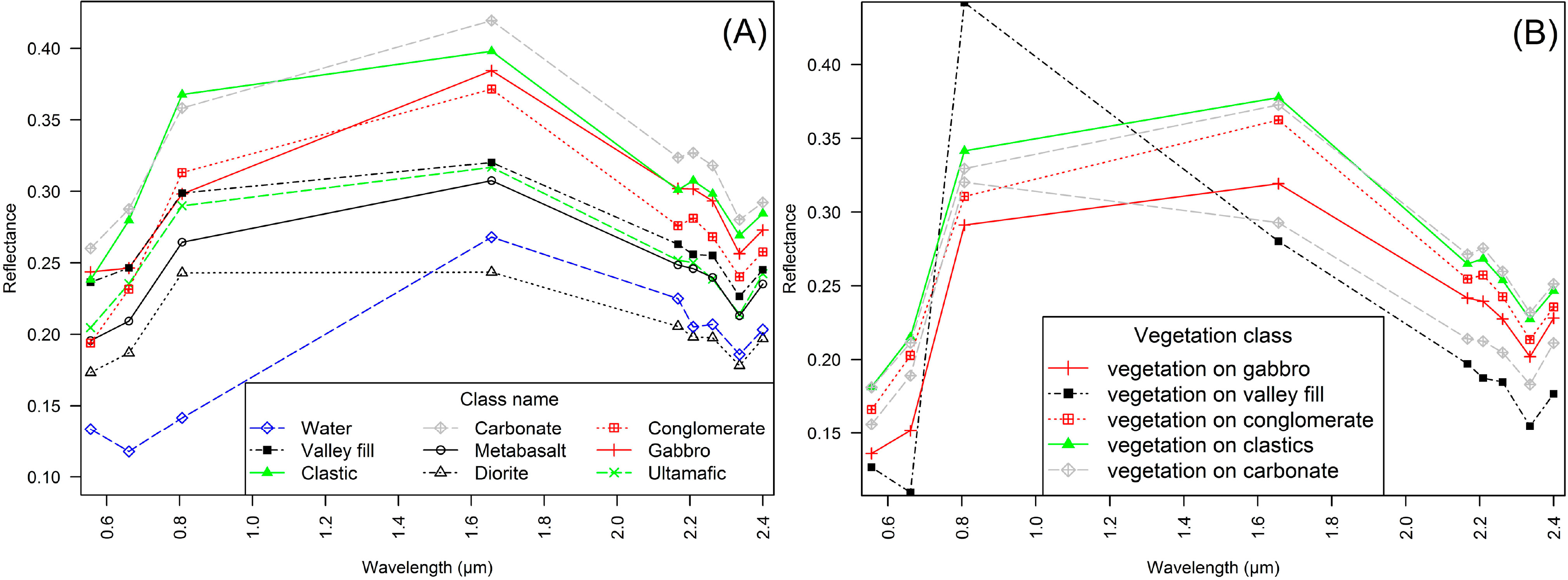
Figures 4, 5, 6A and 6B show the variation of average of all samples for ASTER reflectance, temperature, texture filters (entropy) and SI of the map classes. The average overall reflectance average reflectance of gabbroic rocks is higher than ultramafic and metabasalt rocks, while the average overall reflectance of diorite rocks is lower within the igneous rocks. For the rest classes, the average overall reflectance of the carbonite and the clastics classes are higher than the conglomerate, and the valley fill sediments classes. The carbonate class composed of limestone, calc-schist and marble rocks, which represents the Qulqula radiolarian group, Marble, Calc-schist, Aqra-Bekhme Formation and part of Walash and Naopurdan sequences. The clastics class sources are Tanjero Formation, the lower, the sandstone and the upper units of the Red beds series, which composed of claystones, shales, siltstones, marls, mudstones, and sandstones rock. The source of conglomerate is conglomerate of Red beds series. The valley fill sediments of the Holocene age are named in Figures 4 and 6 and 8 “valley fill”. The average overall reflectance of the water body class is lower than other classes in VNIR bands. All classes have significant absorption in band 8 of ASTER reflectance data. The diorite and valley fill sediments follows a different trend from the other signatures, with enhanced absorption in band 8 (Figure 4A).
We classified the vegetation into five classes as follows (1) vegetation that grew on the valley fill sediments, has a higher reflectance in the NIR band (band 3) than the others; (2) Vegetation that grew on conglomerate; (3) vegetation that grew on clastics rocks; (4) vegetation that grew on carbonate and (5) vegetation on gabbro; which is less dense compared to the other types (Figure 4B).
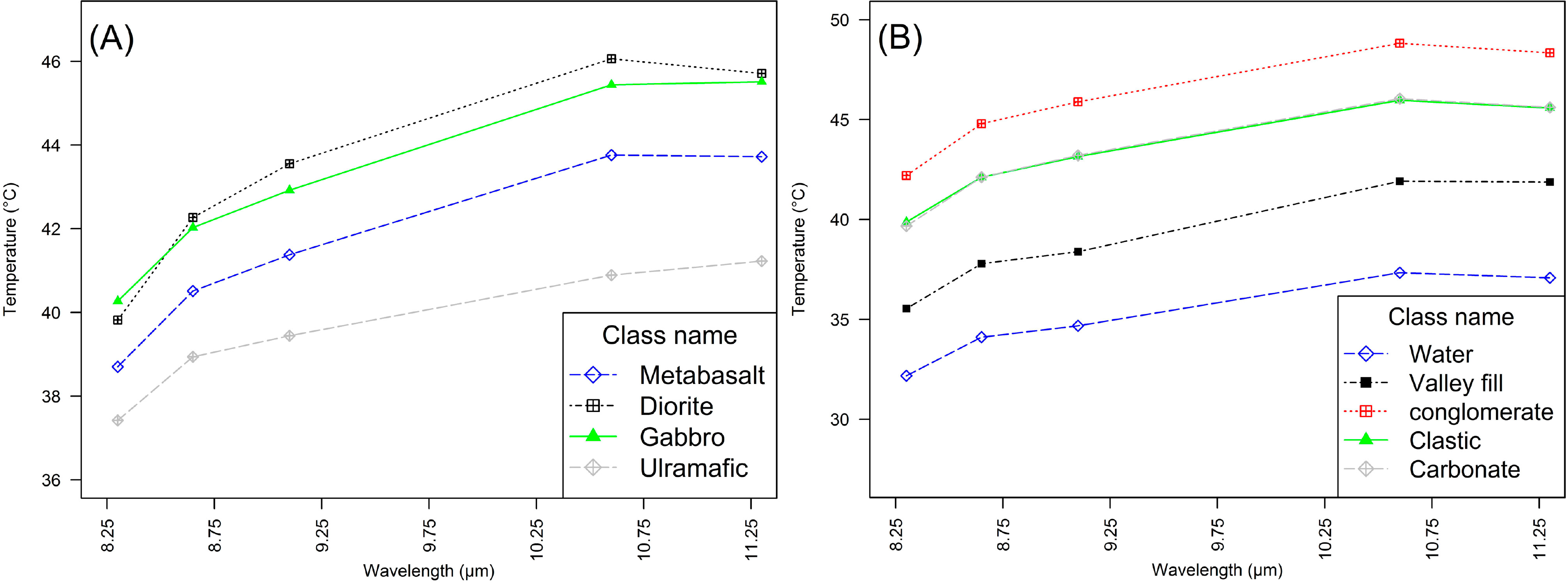
In Figure 5, the at-sensor temperature shows that the ultramafic rocks have average temperature lower than the other igneous rocks. The diorite and gabbro rocks have average temperatures higher than the other igneous rocks. The metabasalt and basalt rocks have moderate average temperatures, especially in the wavelength of 10.6 µm, which is equivalent to band 13 in an ASTER band (Figure 5A). This difference is less in the wavelength of 9.1 µm (band 12 in ASTER). For the non-igneous rock classes, the conglomerate rock has an average temperature higher than the other classes. The water body has an average temperature lower than other classes. The clastics rocks have similar behavior as carbonate rocks as they have approximately the same average temperature. The valley fill sediments have a moderate average temperature (Figure 5B). The temperature of gabbro-diorite, conglomerate, clastic rocks and carbonite rocks are decreasing in the wavelength of 11.3 µm (band 13) more than in the wavelength of 10.6 µm (band 14). All curve in Figure 5 show variations in the temperatures between different wavelengths reach to 5 °C. The maximum temperature located in 10.6 µm, is equivalent to band 13 in an ASTER band.
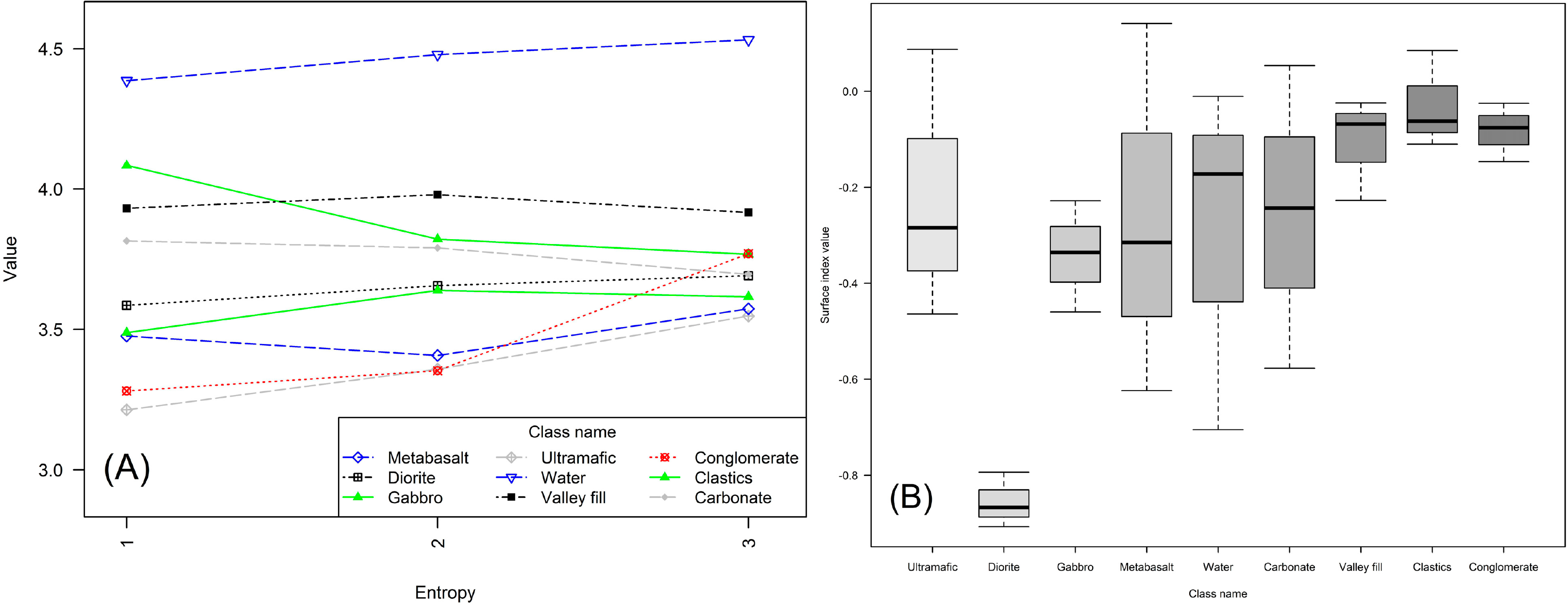
The entropy measures (on band 1, 2 and 3; Figures 6A and 7A) show that the water body has average entropy values higher than the other classes, while the ultramafic rocks have the lowest average entropy values. The SI has high separability and low correlation with the other input dataset used for the classification, where the highest correlation of the SI with the input dataset is 0.21. Figure 6B shows that all boxplots of classes have upper quartile values of the SI < 0. The boxplot interquartile range of the SI for diorite rocks is lower than that of all rocks (Figure 6B). Figure 7B shows that the SI map is clearly discriminated between the igneous (especially diorite and gabbro) and the sedimentary rocks, where the igneous rocks have range values lower than the sedimentary rocks.
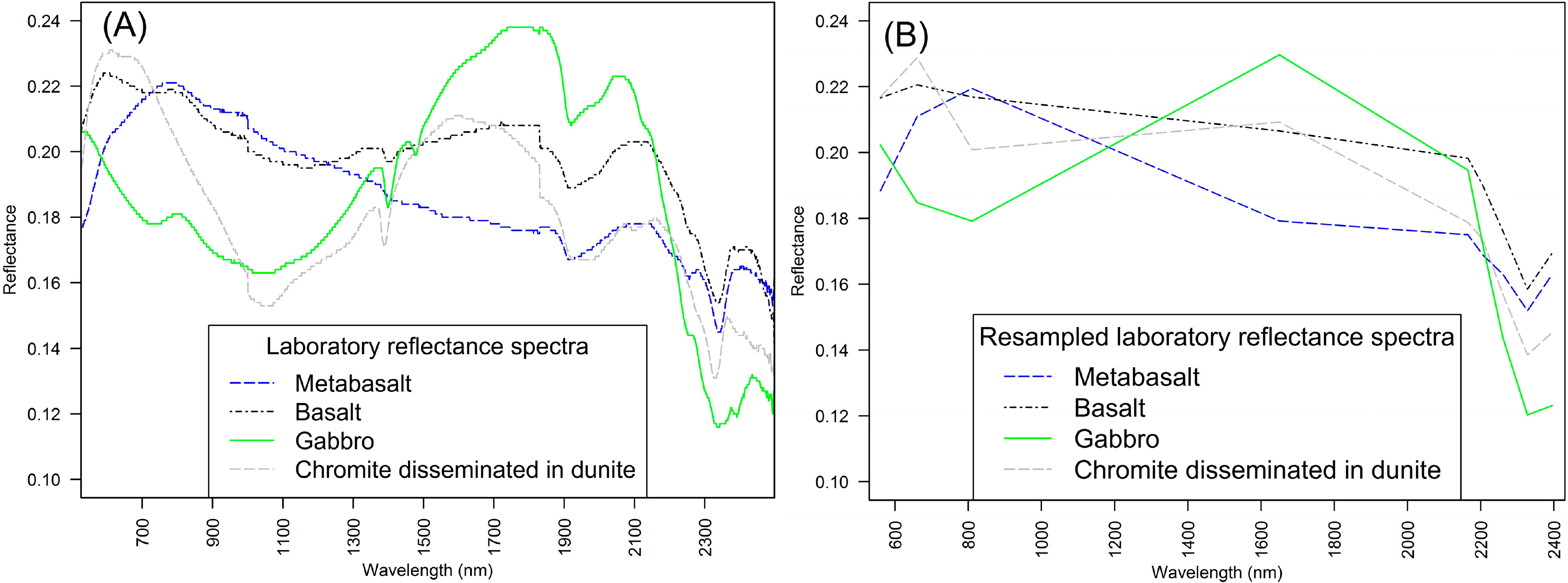
The laboratory reflectance spectra and their respective ASTER-resampled spectra in Figure 8 show that all classes have strong absorption in wavelength 2325 nm (band 8 of ASTER) and 1915 nm. The laboratory spectrum of metabasalt (Figure 8B) has similar behavior as metabasalt endmember (Figure 4A) in all bands expect band 4, which shows less absorption than laboratory spectrum of metabasalt. Metabasalt and basalt have reflectance absorption at a wavelength of 1000 nm and 2250 nm. In addition, basalt has a reflectance absorption at a wavelength of 1400 nm and 1830 nm. The laboratory spectrum of gabbro (Figure 8B) has a similar behavior as the gabbro endmember (Figure 4A) in all bands expect visible bands, where it shows less absorption than the laboratory spectrum of gabbro. Similarly, the laboratory spectrum of ultramafic (Figure 8B) has a similar behavior as the ultramafic end-member (Figure 4A) in all bands expects visible bands, where it shows less absorption than the laboratory spectrum of ultramafic. Gabbro and dunite containing chromite have significant absorption at a wavelength of 1050 nm, which appears in the band 3 of ASTER reflectance data. In addition, dunite containing chromite has a reflectance absorption in wavelength of 1391 nm, and 1830 nm, and gabbro sample has a reflectance absorption at a wavelength of 730 nm, 1400 nm, 1480 nm, 1915–2000 nm and 2250 nm. Gabbro and dunite containing chromite have high reflectance in wavelength 1650 nm and 2150 nm (band 4 and 5 of ASTER reflectance data, respectively), but the gabbroic rock has a higher reflectance than dunite containing chromite rock (Figure 8).
4.2. Improving the Lithological Mapping of the MOC
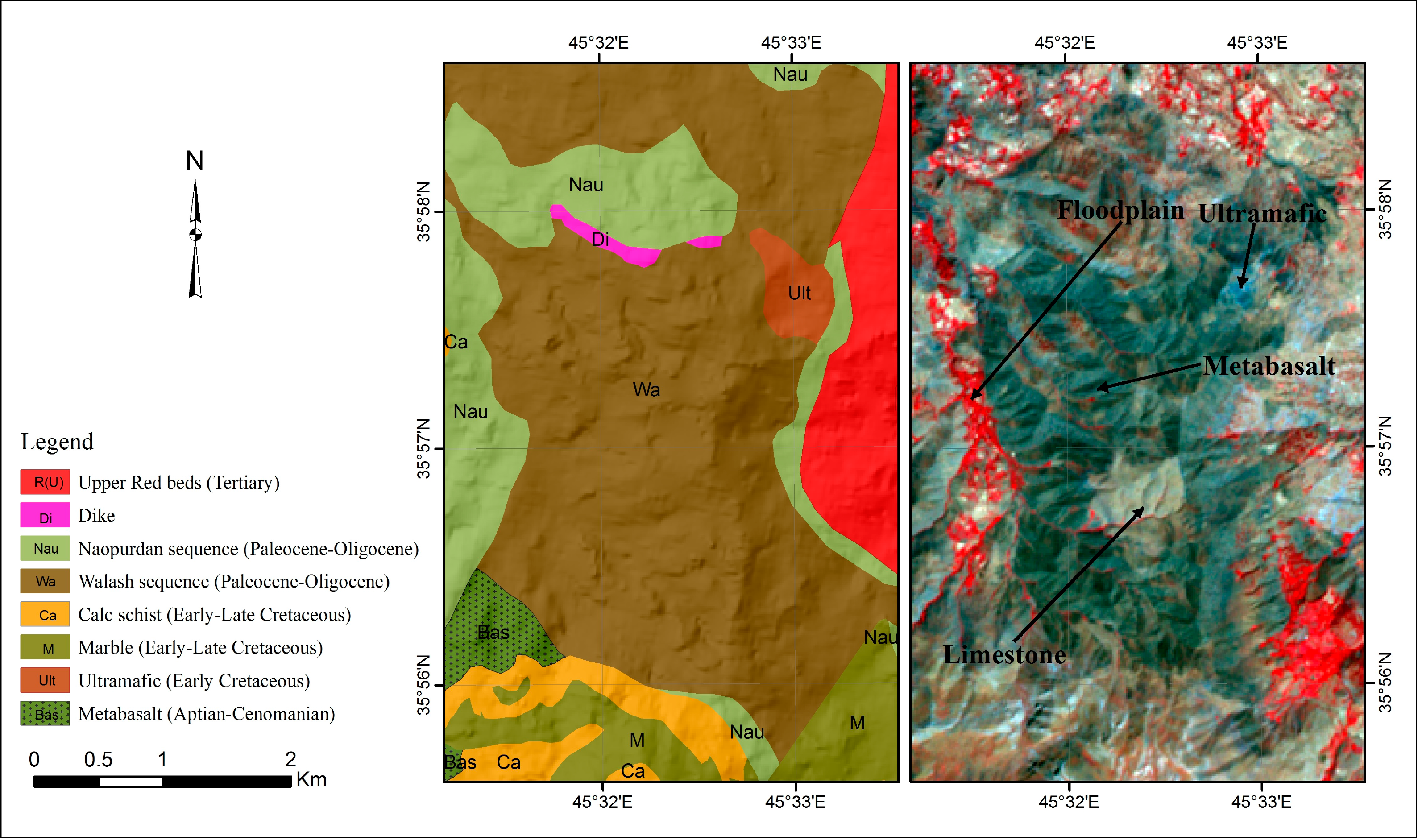
Figure 9 shows a good example of the mismatch between the previous lithological map and ASTER satellite data. The ASTER data show that a big body of the metabasalt with dark green color surrounds the limestone, which has a light gray color. The north part of this continuous body is classified as Walash and Naopurdan sequences in the former map. Healthy vegetation covers the valley fill sediments, (red color in Figure 9), which located in the western part of the metabasalt body are classified as a Walash sequence in the previous map. Figure 10A displays a false color composite image produced from three ASTER bands, where band 3 is assigned to red, band 2 to green and band 1 to blue. As shown in Figure 10A, the gabbro, ultramafic, metabasalt and gabbro to diorite are displayed in blue, spring green, teal and dark green color, respectively. Figure 10B represents the final classified lithological map that is already filtered from a small amount of noise. The two largest classes in the classified lithological map are carbonite class and metabasalt class with an accumulated surface of 148.76 and 129.77 km2, respectively. The smallest is gabbro to diorite class, which covers about 2.17 km2. The water body covers 2.17 km2 and is displayed in black color in R3:G2:B1 of ASTER data. The Lesser Zab River in the north, which runs with the Iraqi-Iranian border, and the Quala Chwalan River in the west of study area belong to water body class. These two rivers have an average width of 40 m. The second new class is valley fill sediments found on both sides of the Quala Chwalan River and the Lesser Zab Rivers in addition to other big valleys. This class covers an area of 18.49 km2.
4.3. Classification Accuracy
Table 2 shows the kappa and overall accuracy for different combination datasets, which implemented using SVM method. Before adding the SI feature, the overall accuracy of the SVM map for the all nine classes is ∼72.8%, the producer and user’s accuracies are ∼62.1% and 63.5% respectively while the kappa coefficient is ∼0.67. When we added SI the overall accuracy reaches ∼80.5%, the producer’s accuracy ∼78.5%, user’s accuracy ∼81% and kappa coefficient 0.739. The overall accuracy is estimated using the contingency error matrix to assess validation (Table 3). The producer’s accuracy and user’s accuracy for each class is illustrated in Table 3 as well. The gabbro to diorite and water classes have the best producer’s accuracy (>90%) and the valley fill sediments and gabbro to diorite classes have the best user’s accuracy (>97.3%). The lowest producer’s accuracy was achieved for the Clastics class (60.27%), while the lowest user’s accuracy was achieved to be 66.38% and 67.69% for the ultramafic and clastics classes, respectively.
4.4. Mineral and Chromite Detection (Fe, Mg)Cr2O4
The radius value of 0.05 has been set to allow an extreme high confidence of detection for the SAM method yielded 13 pixels (which represent <0.0007% of the total pixels). These 13 pixels clustered in two groups represent the expected pixels that have the highest concentrations of chromite. These pixels were converted to points (Figure 11A). One group was accessible for ground truthing. This group is located in the surroundings of field checkpoint MD1 in Figure 11A, and represents a large concentration of chromite. It covers ∼0.3 km2 (300 m × 1000 m). The chromite is coarsely crystalline and of greenish-black color embedded in the dunite host rock, (Figure 12A). Four samples were selected for spectral (Figure 8A) and chemical (MD1; Table 4) analyses. The average chromium concentration is 8.46%. The XRD analysis shows that this rock contains forsterite (Mg2SiO4), and chromite. The chemical and XRD analyses of plagiogranite samples (P; Table 4) show that the rock contains quartz, albite and muscovite with a SiO2 concentration of 79.23%. Field observation shows that dikes e.g. serpentine, plagiogranite dikes (Figure 12B,D) penetrate the basalt and metabasalt rocks.
Figure 12B shows a plagiogranite, which is an acidic dike that has intruded the dunite host rocks near MD1 field checkpoint. The gabbro is medium to coarse grained, occasionally fine-grained (Figure 12C). In many parts of the MOC, the gabbro contains iron ore. The Walash sequence consists of volcanic cones enclosed in limestone and clastics rocks and lacks acidic dikes and serpentine bodies (Figure 12D). The peridotite rocks are the most common ultramafic rocks in the study area and can be easily recognized in the field. Dunite rocks can be found in the ultramafic rocks (surrounds field checkpoint MD1 in Figure 11A).
5. Discussion
Although SVM is an advanced machine learning algorithm used to get optimal solutions for classification problems and may be more accurate than other algorithms [106], this method has not been widely applied for lithological mapping. One of the advantages of SVM it that is allows to classify several layers with different statistical distributions. The SVM approach enables us to discriminate between volcanic and sedimentary rocks within Walash and Naopurdan sequences, whereas these sequences were not differentiated in previous studies [28,42]. Figure 11A shows the volcanic rocks in red color, whereas the sedimentary rocks are illustrated in orange color. The outcrops of volcanic and sedimentary rocks were checked in the field and are backed by previous studies [28,100]. The area from field checkpoint D1 to Sh1 through D3 represents a continuous metabasaltic body that covers > 10 km2 (Figures 11A and 12B). It may represents a part of the volcanic arc of Neotethys in the MOC. The olive green patch in the NW of Figure 11A located between the Iraqi and the Iranian parts was inaccessible to us. Al-Mehaidi [28] mapped the Iraqi part as a Walash sequence, whereas Sadat [29] mapped the Iranian part as a gabbro to diorite with ultramafic inclusions. The signature of this region is different from the signature of Walash and Naopurdan sequences (clastics or volcanic rocks). We thus confirm the interpretation of Sadat [29] for the Iranian part and generalize it to the Iraqi part. Moreover, outcrops of gabbro and diorite start to appear near this area (Figure 11C). The emissivity is directly related to temperature [107], and silica concentration [108]. Therefore, the increase of temperature in the wavelength of 10.6 µm (band 13 of ASTER) can be evidence for the presence of the gabbro-diorite rocks because they have more silica than metabasalt and basalt rocks (Figure 5A). In addition, the decrease of temperature in the wavelength of 11.3 µm (band 14 of ASTER) may be due to the hydroxyl contained in the biotite and hornblende within the diorite. The temperature curve’s behavior of valley fill sediments is similar to the emissivity curve of dark sand provided by Schmugge [109]. The clastic and carbonite rock curves show similarity with the curves provided by Rowan and Mars [110] and Tangestani et al. [22], but in our curves the band 12 has more emissivity than both curves. The mafic and ultramafic rocks curves have less emissivity in band number 10 and 11 compared to the curves provided by Tangestani et al. [22], and Yajima and Yamaguchi [19]. Water curves show less emissivity in band number 10 compared to the curves provided by Lammoglia et al. [111] (Figure 5). The variation of temperatures at different wavelengths for each rock type (Figure 6) is due to the variance in the emissivity, which is affected by chemical content of the rock itself [110].
The rivers in the study area are clear water bodies. Normally, the spectral reflectance of clear water declines constantly after 580 nm [112]. However, the spectral reflectance of water class is higher than standard spectral reflectance clear water, especially in SWIR, because the rivers in the study area are shallow and the bedrock influences the reflectance (Figure 4A). All classes have strong absorption in band 8 because of C-O, hydroxyl and Fe+2 effects [45,113,114]. The trend of valley fill sediments and diorite spectra in bands 7 and 8, which is different than the rest of the spectra indicate hydroxyl bearing minerals. The valley fill sediments spectra are mostly different because of the influence of vegetation. The conglomerates, clastics rocks and calc schist have high absorptions in band 2 and 5 of ASTER data because they include quartz (Figure 4A; [44]). Mafic rocks (i.e., metabasalt and gabbro), which are brighter than ultramafic rocks have reflectance higher than ultramafic rocks in visible bands (Figures 4A and 8). The felsic rocks have a higher temperature than the mafic rocks, but the difference in temperature between both is less in band 9 and 10 of ASTER data (Figure 5A). The same observations can be made for the conglomerate, clastic rocks and calc-schist rocks, which contain a high amount of SiO2 (e.g., SiO2 in calc-schist >45% [28]). The emissivity has an inverse relationship with the water content and this explains the low temperature for the water body class and the valley fill sediments class, which are close to the rivers and become saturated with water. The conglomerates, clastics rocks, carbonite rocks have absorption in band 14 of ASTER data due to the C-O content (Figure 5A; [110]). It was difficult to differentiate the Qulqula radiolarian group and the Aqra-Bekhme Formation because both are composed mainly of limestones and clastic rocks. Therefore, both are mapped as carbonate classes, but there is a narrow outcrop of Red beds (clastics class) that displays a NW-SE trend representing the upper contact of the Aqra-Bekhme Formation (Figure 10B). The high weathering of the Red beds increases its spectrum reflectance [36], that becomes closer to the carbonite rocks spectrum. Therefore, many parts of Red beds do not appear in Figure 10 and that is the reason of a slight decrease of the accuracy of clastic rocks classification (Table 3).
The decrease of the producer’s accuracy for conglomerate class is mainly due to the fact that conglomerate gravels contain metabasalt rocks (Table 3). There is thus an overlap in the ranges of ASTER reflectance between both formations. The second reason is mixing of clastics rocks with conglomerate, which includes clastic sediments as some of the cementing materials. The decrease of the producer and user’s accuracy for the ultramafic and gabbroic rocks is related to their similar chemical composition, especially between gabbro and metabasalt.
The combination of layers from ASTER, textures and geomorphic features increased the accuracy of SVM classification. The significant increase happened when we combined SI to dataset layers, because the SI is sensitive to relative uplift, incision, and occurrence of preserved surfaces. In this study, the refined lithological classification of the MOC has increased of 4.3% when we combined the SI. The better discrimination using SI is because it combines the HI ability for highlighting the flatness of surfaces and SR ability for determining the degree of incision of a surface. The negative values of SI for carbonate and clastics class, ultramafic class, gabbro class and metabasalt class are related to higher valleys dissection than for ultramafic. The low positive values of the SI are related to the higher state of preservation (i.e., less erosion). The Lesser Zab River induces reduction of the values of the SI in the gabbro-diorite body near the Iraqi-Iranian border due to the intense jointing in this body (Figures 6B and 7C).
Texture layers such as the second moment and the three selected layers of the entropy are useful, while the rest of the textures did not show any significant differences (sometimes decreasing in accuracy) when combined them to the dataset. The linear shape of the river and its neighboring floodplain (valley fill sediments; <60 m width, which is smaller than a kernel size) led to increase of entropy values for the water body class and the valley fill sediments class due to their inhomogeneity with the neighbor pixels. The gabbro rocks that are strongly eroded and dissected are also highlighted by high entropy values. The entropy bands help us to increase the discrimination between the metabasalt and conglomerate, where the metabasalt represent the source of conglomerate gravel (Figure 6A). However, the accuracy of the conglomerate classification is still not high (i.e., <71.5 for both Producer’s and user’s; Table 3).
The spectra of MD1 samples show absorptions at wavelengths of 366 nm, 370 nm, 388 nm, 1050 nm and 2000 nm due to the occurrence of Cr3+, Cr2+ and Fe2+ content in chromite [115] (Figure 8A and Table 4). A wide spectrum absorptions region (900–1300 nm) centered in 1050, a broad shallow feature (1900–2072 nm) centered in 1967, and a sharp spectrum absorptions in 1388 nm, 2300 nm and 1831 nm are due to olivine content [13,15,16,21,113,115–118]. Metabasalt, basalt and gabbro reflectance samples spectra have absorptions located at 1000–1050 nm and 1800–1900 nm because of ferrous iron (Fe2+) content [45,119]. All classes have strong absorption in band 8 because of C-O, hydroxyl and Fe+2 effects [45,113,114] (Figure 8A).
SAM method does not consider the spectral illumination and only consider the spectral similarity between the reference and image spectra [120], therefore it introduces potential commission errors in the results. However, the SAM method provides a robust technique to detect chromite in the MOC by setting extremely conservative thresholds. Somehow, the chemical content homogeneity of the big ultramafic bodies contributed to detect the chromite that has low concentrations. In addition, the spectra of ultramafic rocks are closer than other rock types to the chromite spectrum. A likely new chromite body was determined within the dunite host rock and the findings were confirmed by in situ measurements and laboratory analysis.
6. Conclusions
This study demonstrates the potential of the Support Vector Machine (SVM) algorithm for classifying the lithological units of Mawat ophiolite complex, NE Iraq using Advanced Space-borne Thermal Emission and Reflection radiometer (ASTER) satellite data. Various combinations of surface reflectance, at-sensor temperatures, textures and geomorphic parameters were jointly processed using SVM classifications to determine the optimal layers that supply the highest classification accuracy. The best lithological map deriving from a classification without morphological features has a satisfactory overall accuracy of ∼73%. The most determinant spectral variables include surface reflectance, at-sensor temperatures, entropy and second moment layers. The overall accuracy increased to ∼79.3% when we combined the surface index to the spectral variables data set. The surface index allowed a significant increase of the discrimination between the lithological units, especially those that have spectral similarities. The Spectral Angle Mapping (SAM) algorithm was then specifically used to detect chromite occurrences within the ophiolite of Mawat complex. The SAM results contributed to explore a new chromite-bearing body that extends over ∼0.3 km2. The collected samples from fieldwork show that the chromite is coarsely crystalline within the dunite host rocks and the chromium content is 8.46%. The present finding has important implications for starting to explore chromite in the ophiolite regions in Iraq using remote sensing tools. Additional validation work needs to be carried out to estimate the total chromite ore potential in this new location.
In summary, we show that the integration of ASTER data using SVM, its derivative layers such as textures and geomorphic indices such as the surface index is a robust and efficient approach to map complex lithologies in mountainous semi-arid areas. We expect that our work will be a basis for using the geomorphic parameters as a helpful layer to increase lithological classification and enhance the overall mapping performances. Further work needs to concentrate on integrating hyperspectral data with geomorphic parameters to discriminate between different rock units even further.
Acknowledgments
The research was supported by the Ministry of Higher Education and Scientific Research of Iraq (MoHESR), and by the German Academic Exchange Service (DAAD). We are grateful to the Geological Survey of Iraq for providing the data and supporting the fieldwork. In addition, the authors want to thank Ali Taha Yassin and Talal H. Kazem for their help in the completion of fieldwork and Ahmed Tareq Shihab for his assistance with the spectroradiometer.
Author Contributions
Arsalan Ahmed Othman prepared and accomplished the study. He wrote the manuscript. Richard Gloaguen outlined the research, and supported the analysis and discussion. He also supervised the writing of the manuscript at all stages. Both authors checked and revised the manuscript.
Conflicts of Interest
The authors declare no conflict of interest.
References
- Grebby, S.; Cunningham, D.; Naden, J.; Tansey, K. Application of airborne LiDAR data and airborne multispectral imagery to structural mapping of the upper section of the Troodos ophiolite, Cyprus. Int. J. Earth Sci. (Geol. Rundsch) 2012, 101, 1645–1660. [Google Scholar]
- Gad, S.; Kusky, T. ASTER spectral ratioing for lithological mapping in the Arabian-Nubian shield, the Neoproterozoic Wadi Kid area, Sinai, Egypt. Gondwana Res 2007, 11, 326–335. [Google Scholar]
- Grebby, S.; Cunningham, D.; Naden, J.; Tansey, K. Lithological mapping of the Troodos ophiolite, Cyprus, using airborne LiDAR topographic data. Remote Sens. Environ 2010, 114, 713–724. [Google Scholar]
- Moghadam, H.S.; Stern, R.J.; Chiaradia, M.; Rahgoshay, M. Geochemistry and tectonic evolution of the Late Cretaceous Gogher–Baft ophiolite, central Iran. Lithos 2013, 168–169, 33–47. [Google Scholar]
- McQuarrie, N.; Stock, J.M.; Verdel, C.; Wernicke, B.P. Cenozoic evolution of Neotethys and implications for the causes of plate motions. Geophys. Res. Lett 2003, 30. [Google Scholar] [CrossRef]
- Sissakian, V.K. Geological evolution of the Iraqi Mesopotamia Foredeep, inner platform and near surroundings of the Arabian Plate. J. Asian Earth Sci 2013, 72, 152–163. [Google Scholar]
- Xiong, Y.; Khan, S.D.; Mahmood, K.; Sisson, V.B. Lithological mapping of Bela ophiolite with remote-sensing data. Int. J. Remote Sens 2011, 32, 4641–4658. [Google Scholar]
- Gill, R. Igneous Rocks and Processes: A Practical Guide; John Wiley & Sons: West Sussex, UK, 2010. [Google Scholar]
- Jassim, S.Z.; Goff, J.C. Geology of Iraq; Dolin: Brno, Czech, 2006. [Google Scholar]
- Kusky, T.M. Precambrian Ophiolites and Related Rocks; Elsevier: Saint Louis, MO, USA, 2004. [Google Scholar]
- Fouad, S.F. Tectonic Map of Iraq, Scale 1:1,000,000, 3rd ed.; GEOSURV: Baghdad, Iraq, 2010. [Google Scholar]
- Leverington, D.W.; Moon, W.M. Landsat-TM-based discrimination of lithological units associated with the Purtuniq ophiolite, Quebec, Canada. Remote Sens 2012, 4, 1208–1231. [Google Scholar]
- Rajendran, S.; Al-Khirbash, S.; Pracejus, B.; Nasir, S.; Al-Abri, A.H.; Kusky, T.M.; Ghulam, A. ASTER detection of chromite bearing mineralized zones in Semail Ophiolite Massifs of the northern Oman Mountains: Exploration strategy. Ore Geol. Rev 2012, 44, 121–135. [Google Scholar]
- Gül, M.; Gürbüz, K.; Kalelioðlu, Ö. Lithology discrimination in foreland basin with Landsat TM. J. Indian Soc. Remote Sens 2012, 40, 257–269. [Google Scholar]
- Nair, A.; Mathew, G. Lithological discrimination of the Phenaimata felsic–mafic complex, Gujarat, India, using the Advanced Spaceborne Thermal Emission and Reflection Radiometer (ASTER). Int. J. Remote Sens 2011, 33, 198–219. [Google Scholar]
- Amer, R.; Kusky, T.; Ghulam, A. Lithological mapping in the Central Eastern Desert of Egypt using ASTER data. J. Afr. Earth Sci 2010, 56, 75–82. [Google Scholar]
- Ninomiya, Y.; Fu, B.; Cudahy, T.J. Detecting lithology with Advanced Spaceborne Thermal Emission and Reflection Radiometer (ASTER) multispectral thermal infrared “radiance-at-sensor” data. Remote Sens. Environ 2005, 99, 127–139. [Google Scholar]
- Rowan, L.C.; Mars, J.C.; Simpson, C.J. Lithologic mapping of the Mordor, NT, Australia ultramafic complex by using the Advanced Spaceborne Thermal Emission and Reflection Radiometer (ASTER). Remote Sens. Environ 2005, 99, 105–126. [Google Scholar]
- Yajima, T.; Yamaguchi, Y. Geological mapping of the Francistown area in northeastern Botswana by surface temperature and spectral emissivity information derived from Advanced Spaceborne Thermal Emission and Reflection Radiometer (ASTER) thermal infrared data. Ore Geol. Rev 2013, 53, 134–144. [Google Scholar]
- Abedi, M.; Norouzi, G.-H.; Bahroudi, A. Support vector machine for multi-classification of mineral prospectivity areas. Comput. Geosci 2012, 46, 272–283. [Google Scholar]
- Liu, L.; Zhou, J.; Jiang, D.; Zhuang, D.; Mansaray, L.; Zhang, B. Targeting mineral resources with remote sensing and field data in the Xiemisitai area, west Junggar, Xinjiang, China. Remote Sens 2013, 5, 3156–3171. [Google Scholar]
- Tangestani, M.H.; Jaffari, L.; Vincent, R.K.; Sridhar, B.B.M. Spectral characterization and ASTER-based lithological mapping of an ophiolite complex: A case study from Neyriz ophiolite, SW Iran. Remote Sens. Environ 2011, 115, 2243–2254. [Google Scholar]
- Hashim, M.; Pournamdary, M.; Pour, A.B. Processing and interpretation of advanced space-borne thermal emission and reflection radiometer (ASTER) data for lithological mapping in ophiolite complex. Int. J. Phys. Sci 2011, 6, 6410–6421. [Google Scholar]
- Pour, A.B.; Hashim, M. The Earth Observing-1 (EO-1) satellite data for geological mapping, southeastern segment of the Central Iranian Volcanic Belt, Iran. Int. J. Phys. Sci 2011, 6, 7638–7650. [Google Scholar]
- Bolton, C.M.; Lehner, H.P.E.; Mecarthy, M.J. Six Monthly Report July to December, 1954; GEOSURV: Baghdad, Iraq, 1954; p. 158. [Google Scholar]
- Bolton, C.M. Geological Map Kurdistan Series, Scale 1/100000, Sheet k5, Choarta; GEOSURV: Baghdad, Iraq, 1954; p. 32. [Google Scholar]
- Smirnov, V.A.; Nelidov, V.P. Report on 1:200,000 Prospecting-Correlation of the Sulimaniya-Choarta-Penjwin Area Carried out in 1961; GEOSURV: Baghdad, Iraq, 1962; p. 64. [Google Scholar]
- Al-Mehaidi, H.M. Geological Investigation of Mawat-Chuwarta Area, Northeastern Iraq; GEOSURV: Baghdad, Iraq, 1974. [Google Scholar]
- Sadat, M.A.A.N. The Geological Map of Marivan-Baneh Quadrangles, Sheet NI-38–3 (Map No. B5), Scale 1:250000; Geological Survey of Iran: Tehran, Iran, 1993. [Google Scholar]
- Nezhad, J.E. The Geological Map of Mahabad Quadrangles, Sheet NJ-38–15 (Map No. B4), Scale 1:250000; Geological Survey of Iran: Tehran, Iran, 1973. [Google Scholar]
- Andreani, L.; Gloaguen, R.; Shahzad, F. A new set of MATLAB functions (TecDEM toolbox) to analyze erosional stages in landscapes and base-level changes in river profiles. Geophys. Res. Abstr 2014, 16, 16682. [Google Scholar]
- Andreani, L.; Stanek, K.P.; Gloaguen, R.; Krentz, O.; Domínguez-González, L. DEM-based analysis of interactions between tectonics and landscapes in the Ore Mountains and Eger Rift (East Germany and NW Czech Republic). Remote Sens 2014. under revision.. [Google Scholar]
- Mountrakis, G.; Im, J.; Ogole, C. Support vector machines in remote sensing: A review. ISPRS J. Photogramm. Remote Sens 2011, 66, 247–259. [Google Scholar]
- Liesenberg, V.; Gloaguen, R. Evaluating SAR polarization modes at L-band for forest classification purposes in Eastern Amazon, Brazil. Int. J. Appl. Earth Obs. Geoinf 2013, 21, 122–135. [Google Scholar]
- Alavi, M. Tectonics of Zagros Oroginic Belt of Iran: New data and interpretations. Tectonophysics 1994, 229, 221–238. [Google Scholar]
- Alavi, M. Regional stratigraphy of the Zagros Fold—Thrust Belt of Iran and its proforeland evolution. Am. J. Sci 2004, 304, 1–20. [Google Scholar]
- Othman, A.; Gloaguen, R. Automatic extraction and size distribution of landslides in Kurdistan Region, NE Iraq. Remote Sens 2013, 5, 2389–2410. [Google Scholar]
- Othman, A.; Gloaguen, R. River courses affected by landslides and implications for hazard assessment: A high resolution remote sensing case study in NE Iraq–W Iran. Remote Sens 2013, 5, 1024–1044. [Google Scholar]
- Agard, P.; Omrani, J.; Jolivet, L.; Whitechurch, H.; Vrielynck, B.; Spakman, W.; Monié, P.; Meyer, B.; Wortel, R. Zagros orogeny: A subduction-dominated process. Geol. Mag 2011, 148, 692–725. [Google Scholar]
- Lawa, F.A.; Koyi, H.; Ibrahim, A. Tectono-stratigraphic evolution of the NW segment of the Zagros Fold-Thrust Belt, Kurdistan, NE Iraq. J. Pet. Geol 2013, 36, 75–96. [Google Scholar]
- Buday, T.; Suk, M. Report on the Geological Survay in NE Iraq between Halabja and Qala’a Diza; GEOSURV: Baghdad, Iraq, 1978. [Google Scholar]
- Ma’ala, K.A. The geology of Sulaimaniya Quadrangle sheet No. NI-38–3 Scale 1:250,000. In Geological Survey of Iran; GEOSURV: Baghdad, Iraq, 2008; p. 80. [Google Scholar]
- Abrams, M.; Hook, S. ASTER User Handbook (Version 2); Jet Propulsion Laboratory: Pasadena, CA, USA, 2001. [Google Scholar]
- Di Tommaso, I.; Rubinstein, N. Hydrothermal alteration mapping using ASTER data in the Infiernillo porphyry deposit, Argentina. Ore Geol. Rev 2007, 32, 275–290. [Google Scholar]
- Rajendran, S.; Nasir, S.; Kusky, T.M.; Ghulam, A.; Gabr, S.; El-Ghali, M.A.K. Detection of hydrothermal mineralized zones associated with listwaenites in Central Oman using ASTER data. Ore Geol. Rev 2013, 53, 470–488. [Google Scholar]
- Guha, A.; Singh, V.K.; Parveen, R.; Kumar, K.V.; Jeyaseelan, A.T.; Dhanamjaya Rao, E.N. Analysis of ASTER data for mapping bauxite rich pockets within high altitude lateritic bauxite, Jharkhand, India. Int. J. Appl. Earth Obs. Geoinf 2013, 21, 184–194. [Google Scholar]
- Shahzad, F.; Gloaguen, R. TecDEM: A MATLAB based toolbox for tectonic geomorphology, Part 2: Surface dynamics and basin analysis. Comput. Geosci 2011, 37, 261–271. [Google Scholar]
- Environmental Systems Research Institute (ESRI). ArcGIS Desktop: Release 10; Environmental Systems Research Institute: Redlands, CA, USA, 2011. [Google Scholar]
- Analytical Spectral Devices (ASD). RS3; Analytical Spectral Devices: Boulder, CO, USA, 2008. [Google Scholar]
- Analytical Spectral Devices (ASD). ViewSpec Pro; Analytical Spectral Devices: Boulder, CO, USA, 2008. [Google Scholar]
- Susan Moran, M.; Jackson, R.D.; Hart, G.F.; Slater, P.N.; Bartell, R.J.; Biggar, S.F.; Gellman, D.I.; Santer, R.P. Obtaining surface reflectance factors from atmospheric and view angle corrected SPOT-1 HRV data. Remote Sens. Environ 1990, 32, 203–214. [Google Scholar]
- Thome, K.; Biggar, S.; Slater, P. Effects of assumed solar spectral irradiance on intercomparisons of earth-observing sensors. Proc. SPIE 2001. [Google Scholar] [CrossRef]
- Chander, G.; Markham, B.L.; Helder, D.L. Summary of current radiometric calibration coefficients for Landsat MSS, TM, ETM+, and EO-1 ALI sensors. Remote Sens. Environ 2009, 113, 893–903. [Google Scholar]
- Richter, R.; Schläpfer, D. Atmospheric/Topographic Correction for Satellite Imagery; ReSe Applications Schläpfer: Wessling, Germany, 2013; p. 224. [Google Scholar]
- Haralick, R.M.; Shanmugam, K.; Dinstein, I. Textural features for image classification. IEEE Trans. Syst. Man Cybern 1973. [Google Scholar] [CrossRef]
- Vaglio Laurin, G.; Liesenberg, V.; Chen, Q.; Guerriero, L.; Del Frate, F.; Bartolini, A.; Coomes, D.; Wilebore, B.; Lindsell, J.; Valentini, R. Optical and SAR sensor synergies for forest and land cover mapping in a tropical site in West Africa. Int. J. Appl. Earth Obs. Geoinf 2013, 21, 7–16. [Google Scholar]
- Emerson, C.W.; Lam, N.S.N.; Quattrochi, D.A. A comparison of local variance, fractal dimension, and Moran’s I as aids to multispectral image classification. Int. J. Remote Sens 2005, 26, 1575–1588. [Google Scholar]
- Su, W.; Li, J.; Chen, Y.; Liu, Z.; Zhang, J.; Low, T.M.; Suppiah, I.; Hashim, S.A.M. Textural and local spatial statistics for the object-oriented classification of urban areas using high resolution imagery. Int. J. Remote Sens 2008, 29, 3105–3117. [Google Scholar]
- Tsaneva, M.G.; Krezhova, D.D.; Yanev, T.K. Development and testing of a statistical texture model for land cover classification of the Black Sea region with MODIS imagery. Adv. Space Res 2010, 46, 872–878. [Google Scholar]
- Lu, D.; Batistella, M.; Moran, E.; De Miranda, E.E. A comparative study of landsat TM and SPOT HRG images for vegetation classification in the Brazilian Amazon. Photogramm. Eng. Remote Sens 2008, 74, 311–321. [Google Scholar]
- Kumar, T.; Patnaik, C. Discrimination of mangrove forests and characterization of adjoining land cover classes using temporal C-band Synthetic Aperture Radar data: A case study of Sundarbans. Int. J. Appl. Earth Obs. Geoinf 2013, 23, 119–131. [Google Scholar]
- Paneque-Gálvez, J.; Mas, J.-F.; Moré, G.; Cristóbal, J.; Orta-Martínez, M.; Luz, A.C.; Guèze, M.; Macía, M.J.; Reyes-García, V. Enhanced land use/cover classification of heterogeneous tropical landscapes using support vector machines and textural homogeneity. Int. J. Appl. Earth Obs. Geoinf 2013, 23, 372–383. [Google Scholar]
- Mather, P.M.; Tso, B.; Koch, M. An evaluation of Landsat TM spectral data and SAR-derived textural information for lithological discrimination in the Red Sea Hills, Sudan. Int. J. Remote Sens 1998, 19, 587–604. [Google Scholar]
- Dorigo, W.; Lucieer, A.; Podobnikar, T.; Èarni, A. Mapping invasive Fallopia japonica by combined spectral, spatial, and temporal analysis of digital orthophotos. Int. J. Appl. Earth Obs. Geoinf 2012, 19, 185–195. [Google Scholar]
- Ouma, Y.O.; Tetuko, J.; Tateishi, R. Analysis of co-occurrence and discrete wavelet transform textures for differentiation of forest and non-forest vegetation in very-high-resolution optical-sensor imagery. Int. J. Remote Sens 2008, 29, 3417–3456. [Google Scholar]
- Tapiador, F.J.; Avelar, S.; Tavares-Corrêa, C.; Zah, R. Deriving fine-scale socioeconomic information of urban areas using very high-resolution satellite imagery. Int. J. Remote Sens 2011, 32, 6437–6456. [Google Scholar]
- Racoviteanu, A.; Williams, M.W. Decision tree and texture analysis for mapping debris-covered glaciers in the Kangchenjunga area, eastern Himalaya. Remote Sens 2012, 4, 3078–3109. [Google Scholar]
- Pu, R.; Gong, P.; Michishita, R.; Sasagawa, T. Assessment of multi-resolution and multi-sensor data for urban surface temperature retrieval. Remote Sens. Environ 2006, 104, 211–225. [Google Scholar]
- Hack, J.T. Interpretation of erosional topography in humid temperate regions. Am. J. Sci 1960, 258, 80–97. [Google Scholar]
- Willett, S.D.; Brandon, M.T. On steady states in mountain belts. Geology 2002, 30, 175–178. [Google Scholar]
- Pazzaglia, F.J. Landscape evolution models. In Developments in Quaternary Science; Elsevier; Amsterdam, The Netherland: pp. 247–274.
- Matmon, A.; Bierman, P.R.; Larsen, J.; Southworth, S.; Pavich, M.; Caffee, M. Temporally and spatially uniform rates of erosion in the southern Appalachian Great Smoky Mountains. Geology 2003, 31, 155–158. [Google Scholar]
- Burbank, D.W.; Anderson, R.S. Tectonic Geomorphology; Wiley: West Sussex, UK, 2001. [Google Scholar]
- Mather, A.E. Adjustment of a drainage network to capture induced base-level change: An example from the Sorbas Basin, SE Spain. Geomorphology 2000, 34, 271–289. [Google Scholar]
- Mather, A.E.; Harvey, A.M.; Stokes, M. Quantifying long-term catchment changes of alluvial fan systems. Bull. Geol. Soc. Am 2000, 112, 1825–1833. [Google Scholar]
- Gallen, S.F.; Wegmann, K.W.; Bohnenstiehl, D.W.R. Miocene rejuvenation of topographic relief in the southern Appalachians. GSA Today 2013, 23, 4–10. [Google Scholar]
- Lifton, Z.M.; Thackray, G.D.; Van Kirk, R.; Glenn, N.F. Influence of rock strength on the valley morphometry of Big Creek, central Idaho, USA. Geomorphology 2009, 111, 173–181. [Google Scholar]
- Pike, R.J.; Wilson, S.E. Elevation-relief ratio, hypsometric integral, and geomorphic area-altitude analysis. Bull. Geol. Soc. Am 1971, 82, 1079–1084. [Google Scholar]
- Strahler, A.N. Hypsometric (area-altitude) analysis of erosional topography. Geol. Soc. Am. Bull 1952, 63, 1117–1142. [Google Scholar]
- Pérez-Peña, J.V.; Azañón, J.M.; Azor, A. CalHypso: An ArcGIS extension to calculate hypsometric curves and their statistical moments. Applications to drainage basin analysis in SE Spain. Comput. Geosci 2009, 35, 1214–1223. [Google Scholar]
- Grohmann, C.H. Morphometric analysis in geographic information systems: Applications of free software GRASS and R. Comput. Geosci 2004, 30, 1055–1067. [Google Scholar]
- Rouse, J.W.; Haas, R.H.; Schelle, J.A.; Deering, D.W.; Harlan, J.C. Monitoring the Vernal Advancement or Retrogradation of Natural Vegetation; NASA: Greenbelt, MD, USA, 1974. [Google Scholar]
- Vapnik, V.N. The Nature of Statistical Learning Theory, 2nd ed.; Springer: New York, NY, USA, 1999. [Google Scholar]
- Hasan, R.; Ierodiaconou, D.; Monk, J. Evaluation of four supervised learning methods for benthic habitat mapping using backscatter from multi-beam sonar. Remote Sens 2012, 4, 3427–3443. [Google Scholar]
- Colgan, M.; Baldeck, C.; Féret, J.-B.; Asner, G. Mapping savanna tree species at ecosystem scales using support vector machine classification and BRDF correction on airborne hyperspectral and LiDAR data. Remote Sens 2012, 4, 3462–3480. [Google Scholar]
- Zhang, J.; Lin, X.; Ning, X. SVM-based classification of segmented airborne LiDAR point clouds in urban areas. Remote Sens 2013, 5, 3749–3775. [Google Scholar]
- Okujeni, A.; van der Linden, S.; Tits, L.; Somers, B.; Hostert, P. Support vector regression and synthetically mixed training data for quantifying urban land cover. Remote Sens. Environ 2013, 137, 184–197. [Google Scholar]
- Puertas, O.L.; Brenning, A.; Meza, F.J. Balancing misclassification errors of land cover classification maps using support vector machines and Landsat imagery in the Maipo river basin (Central Chile, 1975–2010). Remote Sens. Environ 2013, 137, 112–123. [Google Scholar]
- Brenning, A.; Long, S.; Fieguth, P. Detecting rock glacier flow structures using Gabor filters and IKONOS imagery. Remote Sens. Environ 2012, 125, 227–237. [Google Scholar]
- Huang, C.; Davis, L.S.; Townshend, J.R.G. An assessment of support vector machines for land cover classification. Int. J. Remote Sens 2002, 23, 725–749. [Google Scholar]
- Heumann, B.W. An object-based classification of Mangroves using a hybrid decision tree—Support vector machine approach. Remote Sens 2011, 3, 2440–2460. [Google Scholar]
- Yu, L.; Porwal, A.; Holden, E.-J.; Dentith, M.C. Towards automatic lithological classification from remote sensing data using support vector machines. Comput. Geosci 2012, 45, 229–239. [Google Scholar]
- Yang, X. Parameterizing support vector machines for land cover classification. Photogramm. Eng. Remote Sens 2011, 77, 27–38. [Google Scholar]
- Cohen, J. A coefficient of agreement of nominal scales. Psychol. Meas 1960, 2, 37–46. [Google Scholar]
- Congalton, R.G. A review of assessing the accuracy of classifications of remotely sensed data. Remote Sens. Environ 1991, 37, 35–46. [Google Scholar]
- Pignatti, S.; Cavalli, R.M.; Cuomo, V.; Fusilli, L.; Pascucci, S.; Poscolieri, M.; Santini, F. Evaluating Hyperion capability for land cover mapping in a fragmented ecosystem: Pollino National Park, Italy. Remote Sens. Environ 2009, 113, 622–634. [Google Scholar]
- Brown, D.G.; Lusch, D.P.; Duda, K.A. Supervised classification of types of glaciated landscapes using digital elevation data. Geomorphology 1998, 21, 233–250. [Google Scholar]
- Grebby, S.; Naden, J.; Cunningham, D.; Tansey, K. Integrating airborne multispectral imagery and airborne LiDAR data for enhanced lithological mapping in vegetated terrain. Remote Sens. Environ 2011, 115, 214–226. [Google Scholar]
- Yassin, A.T.; Sammad, F.F.A.; Rahman, R.M.A.; Jabar, M.F.A. Microscopy Study for Copper Mineralization of Mawat Ophiolite Complex. NE Iraq; GEOSURV: Baghdad, Iraq, 2011. [Google Scholar]
- Aswad, K.J.A.; Al-Samman, A.H.M.; Aziz, N.R.H.; Koyi, A.M.A. The geochronology and petrogenesis of Walash volcanic rocks, Mawat nappes: Constraints on the evolution of the northwestern Zagros suture zone, Kurdistan Region, Iraq. Arab J. Geosci 2013, 7, 1403–1432. [Google Scholar]
- Chandrasekar, N.; Mujabar, P.S.; Rajamanickam, G.V. Investigation of heavy-mineral deposits using multispectral satellite data. Int. J. Remote Sens 2011, 32, 8641–8655. [Google Scholar]
- Kruse, F.A.; Lefkoff, A.B.; Boardman, J.W.; Heidebrecht, K.B.; Shapiro, A.T.; Barloon, P.J.; Goetz, A.F.H. The spectral image processing system (SIPS)—Interactive visualization and analysis of imaging spectrometer data. Remote Sens. Environ 1993, 44, 145–163. [Google Scholar]
- Murphy, R.J.; Monteiro, S.T.; Schneider, S. Evaluating classification techniques for mapping vertical geology using field-based hyperspectral sensors. IEEE Trans. Geosci. Remote Sens 2012, 50, 3066–3080. [Google Scholar]
- Clark, R.N.; Swayze, G.A.; Gallagher, A.J.; King, T.V.V.; Calvin, W.M. The US Geological Survey, Digital Spectral Reflectance Library: Version 1: 0.2 to 3.0 Microns; The U.S. Geological Survey: Denver, CO, USA, 1993. [Google Scholar]
- Pal, S.K.; Majumdar, T.J.; Bhattacharya, A.K.; Bhattacharyya, R. Utilization of landsat ETM+ data for mineral-occurrences mapping over Dalma and Dhanjori, Jharkhand, India: An advanced spectral analysis approach. Int. J. Remote Sens 2011, 32, 4023–4040. [Google Scholar]
- Huang, C.; Song, K.; Kim, S.; Townshend, J.R.G.; Davis, P.; Masek, J.G.; Goward, S.N. Use of a dark object concept and support vector machines to automate forest cover change analysis. Remote Sens. Environ 2008, 112, 970–985. [Google Scholar]
- Majumdar, T.J.; Pal, S.K.; Bhattacharya, A. Generation of emissivity and land surface temperature maps using MODIS TIR data for lithological mapping over the Singhbhum-Orissa Craton. J. Geol. Soc. India 2012, 80, 685–699. [Google Scholar]
- Rajendran, S.; Hersi, O.; Al-Harthy, A.; Al-Wardi, M.; El-Ghali, M.; Al-Abri, A. Capability of advanced spaceborne thermal emission and reflection radiometer (ASTER) on discrimination of carbonates and associated rocks and mineral identification of eastern mountain region (Saih Hatat window) of Sultanate of Oman. Carbonates Evaporites 2011, 26, 351–364. [Google Scholar]
- Schmugge, T.; French, A.; Ritchie, J.C.; Rango, A.; Pelgrum, H. Temperature and emissivity separation from multispectral thermal infrared observations. Remote Sens. Environ 2002, 79, 189–198. [Google Scholar]
- Rowan, L.C.; Mars, J.C. Lithologic mapping in the Mountain Pass, California area using Advanced Spaceborne Thermal Emission and Reflection Radiometer (ASTER) data. Remote Sens. Environ 2003, 84, 350–366. [Google Scholar]
- Lammoglia, T.; de Souza Filho, C.R. Spectroscopic characterization of oils yielded from Brazilian offshore basins: Potential applications of remote sensing. Remote Sens. Environ 2011, 115, 2525–2535. [Google Scholar]
- Jensen, J.R. Remote Sensing of the Environment: An Earth Resource Perspective; Pearson Prentice Hall: Upper Saddle River, NJ, USA, 2007. [Google Scholar]
- Abrams, M.J.; Rothery, D.A.; Pontual, A. Mapping in the Oman ophiolite using enhanced Landsat Thematic Mapper images. Tectonophysics 1988, 151, 387–401. [Google Scholar]
- Mars, J.C.; Rowan, L.C. Spectral assessment of new ASTER SWIR surface reflectance data products for spectroscopic mapping of rocks and minerals. Remote Sens. Environ 2010, 114, 2011–2025. [Google Scholar]
- Cloutis, E.A.; Sunshine, J.M.; Morris, R.V. Spectral reflectance-compositional properties of spinels and chromites: Implications for planetary remote sensing and geothermometry. Meteorit. Planet. Sci 2004, 39, 545–565. [Google Scholar]
- Hunt, G. Spectral signatures of particulate minerals in the visible and near infrared. Geophysics 1977, 42, 501–513. [Google Scholar]
- Hunt, G.; Evarts, R. The use of near-infrared spectroscopy to determine the degree of serpentinization of ultramafic rocks. Geophysics 1981, 46, 316–321. [Google Scholar]
- Rowan, L.C.; Simpson, C.J.; Mars, J.C. Hyperspectral analysis of the ultramafic complex and adjacent lithologies at Mordor, NT, Australia. Remote Sens. Environ 2004, 91, 419–431. [Google Scholar]
- Ulmer, G.C.; White, W.B. Existence of chromous ion in the spinel solid solution series FeCr2O4-MgCr2O4. J. Am. Ceram. Soc 1966, 49, 50–51. [Google Scholar]
- Sadeghi, B.; Khalajmasoumi, M.; Afzal, P.; Moarefvand, P.; Yasrebi, A.B.; Wetherelt, A.; Foster, P.; Ziazarifi, A. Using ETM+ and ASTER sensors to identify iron occurrences in the Esfordi 1:100,000 mapping sheet of Central Iran. J. Afr. Earth Sci 2013, 85, 103–114. [Google Scholar]


| Characteristics | VNIR | SWIR | TIR |
|---|---|---|---|
| Band’s Number with Spectral Range (μm) | Band 01: 0.52–0.60 Nadir looking | Band 04: 1.60–1.70 | Band 10: 8.125–8.475 |
| Band 02: 0.63–0.69 Nadir looking | Band 05: 2.145–2.185 | Band 11: 8.475–8.825 | |
| Band 03: 0.76–0.86 Nadir looking (N) | Band 06: 2.185–2.225 | Band 12: 8.925–9.275 | |
| Band 03: 0.76–0.86 Backward looking (B) | Band 07: 2.235–2.285 | Band 13: 10.25–10.95 | |
| Band 08: 2.295–2.365 | Band 14: 10.95–11.65 | ||
| Band 09: 2.360–2.430 | |||
| Spatial Resolution (m) | 15 | 30 | 90 |
| Radiometric Resolution (bits) | 8 | 8 | 12 |
| Dataset Used | Overall Accuracy | Kappa |
|---|---|---|
| ASTER, Entropy (1,2 and 3), Second Moment (1 and 2), Temperature and SI | 79.28 | 0.739 |
| ASTER, Entropy (1,2 and 3), Second Moment (1 and 2) and Temperature | 72.83 | 0.666 |
| ASTER, Entropy, Second Moment and Temperature | 64.91 | 0.582 |
| ASTER, Second Moment and Temperature | 64.76 | 0.575 |
| ASTER, Entropy and Temperature | 63.59 | 0.565 |
| ASTER and Second Moment | 63.84 | 0.564 |
| ASTER | 60.23 | 0.531 |
| Class | Area (km2) | Producer’s Accuracy | User’s Accuracy | Overall Accuracy | Kappa |
|---|---|---|---|---|---|
| Clastics | 14.54 | 60.27 | 67.69 | ||
| Conglomerate | 8.07 | 63.64 | 71.43 | ||
| Gabbro to diorite | 4.82 | 93.75 | 97.30 | ||
| Valley fill sediments | 18.49 | 87.23 | 98.4 | ||
| Gabbro | 61.9 | 73.97 | 78.42 | ||
| Carbonite | 148.76 | 79.18 | 79.18 | ||
| Metabasalt and basalt | 129.77 | 83.19 | 77.59 | ||
| Ultramafic | 33.93 | 68.12 | 66.38 | ||
| Water body | 2.17 | 96.97 | 88.89 | ||
| Total | 422.45 | 78.45 | 80.59 | 79.28 | 0.74 |
| Sample no. | SiO2% | Fe2O3% | Al2O3% | TiO2% | CaO% | MgO% | SO3% | Na2O% | K2O% | Cr2O3 |
|---|---|---|---|---|---|---|---|---|---|---|
| MD1 | 36.16 | 9.01 | 1.99 | 0.03 | 0.26 | 43.31 | 0.16 | <0.02 | 0.1 | 8.46% |
| P | 79.23 | 1.55 | 12.35 | 0.14 | 0.32 | 0.28 | 0.08 | 4.2 | 1.19 | <10 ppm |
© 2014 by the authors; licensee MDPI, Basel, Switzerland This article is an open access article distributed under the terms and conditions of the Creative Commons Attribution license (http://creativecommons.org/licenses/by/3.0/).
Share and Cite
Othman, A.A.; Gloaguen, R. Improving Lithological Mapping by SVM Classification of Spectral and Morphological Features: The Discovery of a New Chromite Body in the Mawat Ophiolite Complex (Kurdistan, NE Iraq). Remote Sens. 2014, 6, 6867-6896. https://doi.org/10.3390/rs6086867
Othman AA, Gloaguen R. Improving Lithological Mapping by SVM Classification of Spectral and Morphological Features: The Discovery of a New Chromite Body in the Mawat Ophiolite Complex (Kurdistan, NE Iraq). Remote Sensing. 2014; 6(8):6867-6896. https://doi.org/10.3390/rs6086867
Chicago/Turabian StyleOthman, Arsalan A., and Richard Gloaguen. 2014. "Improving Lithological Mapping by SVM Classification of Spectral and Morphological Features: The Discovery of a New Chromite Body in the Mawat Ophiolite Complex (Kurdistan, NE Iraq)" Remote Sensing 6, no. 8: 6867-6896. https://doi.org/10.3390/rs6086867