Towards the Improvement of Blue Water Evapotranspiration Estimates by Combining Remote Sensing and Model Simulation

 , and
, and
Abstract
: The estimation of evapotranspiration of blue water (ETb) from farmlands, due to irrigation, is crucial to improve water management, especially in regions where water resources are scarce. Large scale ETb was previously obtained, based on the differences between remote sensing derived actual ET and values simulated from the Global Land Data Assimilation System (GLDAS). In this paper, we improve on the previous approach by enhancing the classification scheme employed so that it represents regions with common hydrometeorological conditions. Bias between the two data sets for reference areas (non-irrigated croplands) were identified per class, and used to adjust the remote sensing products. Different classifiers were compared and evaluated based on the generated bias curves per class and their variability. The results in Europe show that the k-means classifier was better suited to identify the bias curves per class, capturing the dynamic range of these curves and minimizing their variability within each corresponding class. The method was applied in Africa and the classification and bias results were consistent with the findings in Europe. The ETb results were compared with existing literature and provided differences up to 50 mm/year in Europe, while the comparison in Africa was found to be highly influenced by the assigned cover type and the heterogeneity of the pixel. Although further research is needed to fully understand the ETb values found, this paper shows a more robust approach to classify and characterize the bias between the two sets of ET data.
1. Introduction
Water management in agriculture has been always important, especially in areas where water resources are scarce. In this context, it is relevant to distinguish between the sources of the usage: water supplied by precipitation (called green water) and irrigation (called blue water).
Recent studies obtained blue and green water usage in agriculture at large scale, using data from national agricultural statistics, reports and climatic databases, and making use of hydrological models based on the calculation of actual evapotranspiration (ETactual) [1–4]. Moreover, several studies tackled the problem of retrieving global irrigated areas by using national statistics of areas equipped for irrigation [5] and by statistically analyzing remote sensing products [6].
The potential of using remote sensing data for global studies of green and blue waters use and water footprint estimations is discussed in Romaguera et al. [7]. The first approaches to exploit those data at large scale are shown in Romaguera et al. [8,9], where the use of the different components of the water cycle is explored, together with the use of land surface models. Other works used remote sensing to evaluate irrigation performance at regional scale [10–12].
In particular, Romaguera et al. [8] obtained large scale blue water evapotranspiration (ETb), i.e., due to irrigation, based on the differences between remote sensing ETactual obtained from the Meteosat Second Generation (MSG) satellites [13] and ETactual values simulated from the Global Land Data Assimilation System (GLDAS) [14]. In general, it was found that there was a systematic bias between the two datasets in rain-fed pixels and that this difference was variable in time and space. The bias amplitude changed along the year, roughly resembling a positive concave curve. The maximum amplitude value reached up to 3 mm/day and occurred in the months of spring and summer in northern latitudes. The spatial variability of the bias was associated in this paper to vegetation characteristics and the remote sensing observation angle. Romaguera et al. [8] calculated the bias per day and used three parameters to generate a classification map for Europe to discriminate areas with different bias patterns: the maximum value of the NDVI (NDVImax), the season where NDVImax occurred, and the viewing zenith angle (VZA) of the sensor on board MSG. Thresholds were assigned to distinguish between classes. Recent work from Romaguera et al. [15] showed that the classification scheme was not sufficient to describe the variability of the bias estimates in the continent of Africa and proposed the inclusion of a climatic indicator in the selection of parameters for the classification.
Similar results in terms of bias between these two datasets were obtained by Ghilain et al. [13] and the validation report from the Land Surface Analysis Satellite Applications Facility (LSA–SAF) [16], who showed that the bias might be explained by the differences in the inputs of incoming solar radiation, the ratio between leaf are index (LAI) and stomatal resistance, and land cover type. Yilmaz et al. [17] identified discrepancies in insolation inputs and analyzed differences in soil moisture, when comparing these data sets in the region of the Nile River basin. Romaguera et al. [8] emphasized that the GLDAS simulations did not account for extra water supply due to irrigation and consequently it was expected that they underestimate ETactual during the cropping season in irrigated areas. Therefore in the aforementioned work, the differences between these two estimates were corrected for the bias in rain–fed croplands, to obtain blue water evapotranspiration according to:
ΔET is the difference between MSG ETactual (MSG–ET in the following) and GLDAS ETactual (GLDAS–ET in the following), and bias is this difference in ETactual calculated in reference areas, i.e., rain–fed croplands where irrigation practices are not present.
In this paper, we intend to solve the drawbacks of the previous methodology by improving the classification scheme in order to achieve a better spatial representation of the bias in rain–fed croplands, which results in better estimates of ETb.
First, a better choice of parameters is proposed to represent regions with common hydrometeorological conditions, based on three processes at which ETactual estimation may be affected, namely vegetation characterization, atmosphere/forcing definition, and land–atmosphere interaction. Secondly, an alternative strategy for classification is adopted, based on the use of classifiers, instead of the selection of thresholds published in the aforementioned work. This makes the methodology generic and robust. The suitability of these classifiers is explored via the classification maps and the bias curves obtained per class.
Section 2 explains the selection of parameters for the classification and the properties of the selected classifiers. Next, in Section 3, the datasets used in this paper are detailed. The Results section includes the classification maps, the bias curves and ETb outputs compared with the original methodology. The application of the method to the region of Africa is shown in Section 5, together with the comparison of the results with existing literature. Finally relevant issues about the proposed improved methodology can be found in the Discussion and Conclusions sections.
2. Method
The objective of this work is to improve the existing methodology for ETb estimation [8] on two aspects: the selection of parameters for the classification of the study area and the classification method.
2.1. Selection of Parameters for the Classification
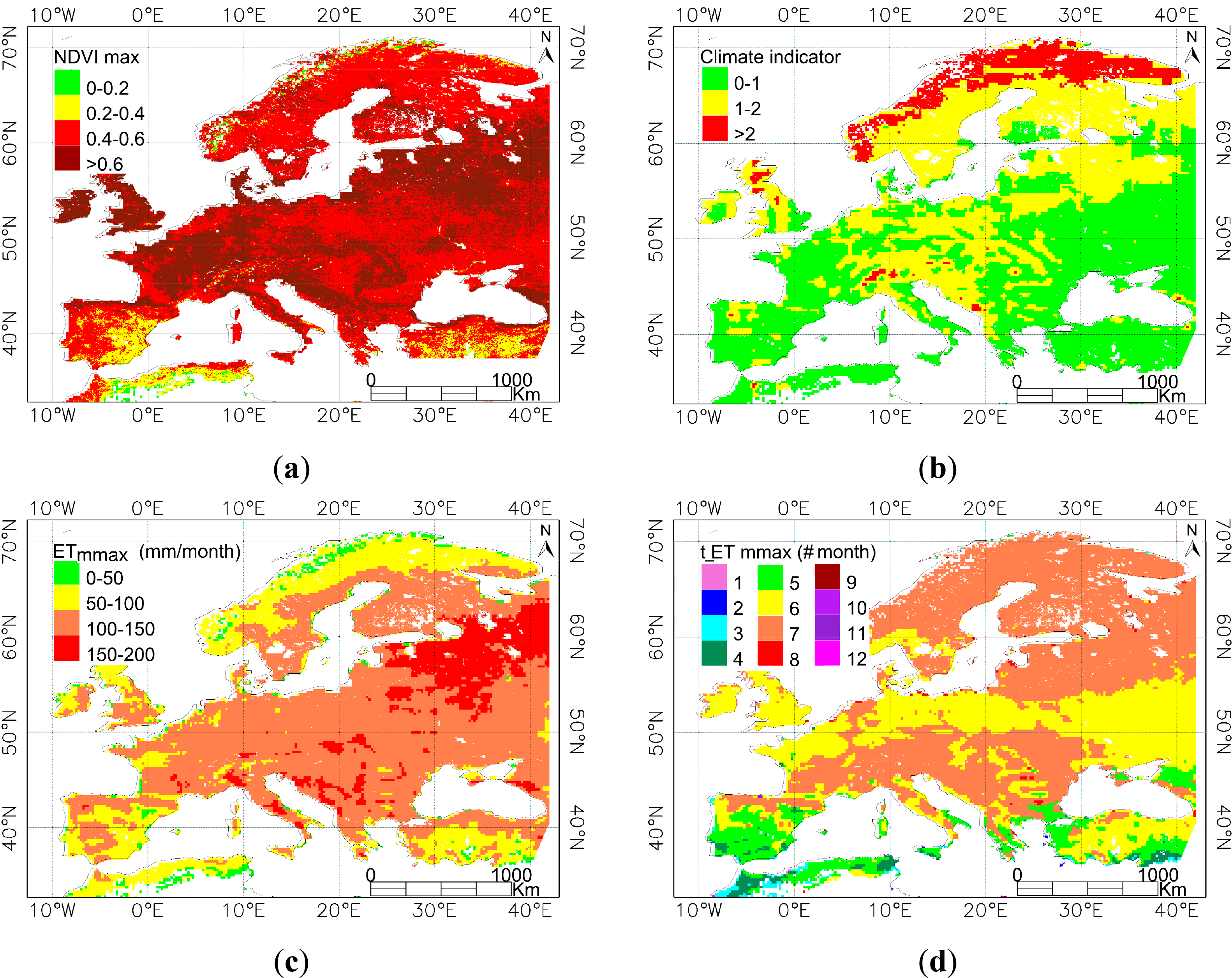
The hypothesis here is that the classification output discriminates between areas with different bias curves, i.e., differences along the year of MSG–ET and GLDAS–ET estimates. Therefore, potential variables need to be identified in order to explain the differences in ETactual retrievals. In the present work, a more complete selection of parameters is carried out by accounting for three processes at which ETactual estimation from both sources may differ, namely vegetation characterization, atmosphere/forcing definition and land–atmosphere interaction. In order to account for the vegetation properties, a typical indicator is selected, the NDVI, and in particular its maximum value along the year, NDVImax. Precipitation and net radiation are combined into a climatic indicator (CI) to account for the driving forces for ETactual, as follows [18]:
The land–atmosphere interaction is included in the selection of parameters by means of the monthly accumulated ETactual, and in particular the maximum value along the year (ETmmax). This aggregated value is chosen in order to reduce relative errors in ETactual estimation. Since the focus of this paper is to obtain the ET bias curves per class, including ET itself in the classification inputs contributes to capture the observed variability. Moreover, as shown in previous literature [8,13], a seasonality was found in this bias. The position of the bias maxima was variable and, therefore, it was reasonable to select t_ETmmax (month when ET monthly maxima occurs) to account for these different patterns.
Being aware that other potential variables might have been included in this selection, such as land surface temperature and albedo, effective precipitation, soil moisture, LAI or topography, the number was limited in order to reduce data redundancy when the parameters were correlated or equivalent in terms of climate and vegetation interaction. Moreover, the use of too many variables in a classification procedure may decrease the classification accuracy [19].
2.2. Classification Methods
Many classification methods exist in the literature and all have their own merits. However, the question of which classification approach is suitable for a specific study is not easy to answer [20]. Romaguera et al. [8] used a basic classification method, based on thresholds, as follows: NDVImax higher/lower than 0.4, October to March and April to September periods for the NDVImax to occur, and VZA intervals of 10°.
In this paper, the use of three different classifiers was explored and discussed. Firstly, a common classification approach was chosen: an unsupervised classification based on k–means. Secondly, a more advanced learning method was selected: an unsupervised classification based on the expectation–maximization algorithm. These two approaches do not use training samples, they work per pixel, they are hard classifiers (i.e., output is a definitive decision) and they do not use spatially neighboring pixel information for the classification, all aspects that are appropriate to this study. Thirdly, an image transform of the selected parameters was carried out by using the principal component analysis in order to reduce data redundancy of correlated bands and concentrate the information contents in the transformed images, exploring the possible clustering.
2.2.1. Unsupervised Classification Based on K–means
An unsupervised classification of the study area was executed in order to cluster pixels based on the k–means statistical technique [21]. This method calculates initial mass means evenly distributed in the data space and then iteratively clusters the pixels into the nearest class using a minimum distance technique. In each iteration, classes’ means are recalculated and pixels are reclassified with respect to the new means. All pixels are classified to the nearest class unless a standard deviation or distance threshold is specified, in which case some pixels may be unclassified if they do not meet the selected criteria. This process continues until the number of pixels in each class changes by less than the selected pixel change threshold or the maximum number of iterations is reached. The four-layer input file contained NDVImax, ETmmax, t_ ETmmax and CI as described in the previous section. A maximum of 100 iterations was fixed to ensure completion of the algorithm, and the default value of 5% was conserved for the pixel change threshold [22].
Neither standard deviation, nor distance thresholds were fixed. In order to select the optimal number of clusters and to evaluate the clustering found by the algorithm, a scattering distance (SD) quality index was calculated according to Rezaee et al. [23], which accounts for the intra–cluster and inter–cluster distances as:
A small value of Scat(c) indicates a compact cluster. The second term Dis(c) is influenced by the geometry of the cluster centers and increases with the number of clusters. The optimal value for the number of clusters present in the data set is such that minimizes the SD index.
In the present research, the maximum number of clusters for the unsupervised classification was set to 20, assuming a reasonable minimum percentage of pixels per class of 5%. The classification was obtained for 5 up to 10 clusters and SD was calculated. As a result, the number of clusters for which the SD quality index was minimized was found to be 6 in the region of Europe.
2.2.2. Unsupervised Classification Based on the Expectation–Maximization Algorithm (EM)
The Expectation–Maximization algorithm [24] is an iterative procedure that estimates the probabilities of the elements to belong to a certain class, based on the principle of maximum likelihood of unobserved variables in statistical models. The EM iteration alternates between performing an expectation (E) step, which creates a function for the expectation of the log–likelihood evaluated using the current estimate for the parameters, and a maximization (M) step, that computes parameters maximizing the expected log–likelihood found on the E step. These parameter estimates are then used to determine the distribution of the latent variables in the next E step. This classification was performed using the machine learning software WEKA version 3.6.9 (Waikato Environment for Knowledge Analysis) [25], using the implemented Simple EM classifier. This software contains tools and algorithms for the analysis of data and predictive modeling, where the system is trained and can learn from the data and provide classified outputs. EM assigns a probability distribution to each instance which indicates the probability of it belonging to each of the cluster and can decide how many clusters to create by cross validation. In the current research, the maximum number of iterations was set to 100 to ensure completion of the algorithm. Moreover, the software allowed to test the model output by using the 66% of the data as a training set and the rest for testing.
2.2.3. Classification Using Principal Component Analysis (PCA)
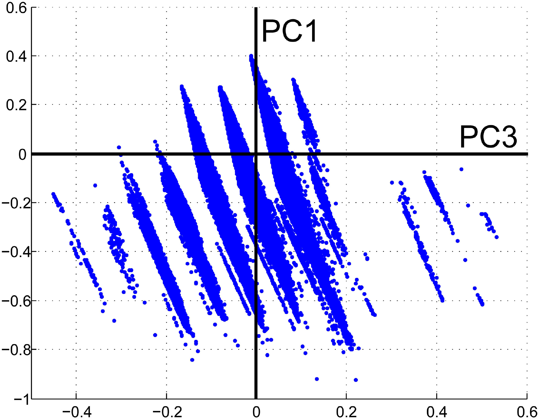
The principal component analysis (PCA) [26] consists of a transformation of the input dataset (multilayer file with NDVImax, ETmmax, t_ETmmax and CI) to produce uncorrelated output bands, segregate noise components, and reduce the dimensionality of data sets. The characteristic matrix (covariance matrix or correlation matrix) of the variables, the eigen values, the eigen vectors (which are the directions of the principal components (PC)), and the coordinates of each data point in the direction of the PC’s were calculated. A new set of orthogonal axes was found, which had their origin at the data mean and which were rotated so the data variance was maximized. PC output bands were linear combinations of the original spectral bands and were uncorrelated. The relationships found between the principal components, which led to the clustering of the data are shown in the results section.
3. Data Sets
Table 1 describes the main characteristics of the datasets used in the present work which are detailed in the following subsections.
From a technical point of view, the combination of data of different spatial resolution, extent and geographical projection was tackled by creating a layer stack where the data were resampled and re–projected to a common output projection. The present work was carried out at the resolution of the MSG–ET products.
3.1. Evapotranspiration and Cover Type Data
Based on Equation (1), the main datasets for obtaining the ETb were the ETactual products from the MSG satellites provided by the Land Surface Analysis Satellite Applications Facility (LSA–SAF) [13] (MSG–ET) and ETactual from the Global Land Data Assimilation System (GLDAS) generated with the Noah land surface model [27,28] (GLDAS–ET). These datasets are available from the LSA–SAF website ( http://landsaf.meteo.pt/) and the NASA Goddard Earth Sciences Data and Information Services Center (GES DISC) ( http://disc.sci.gsfc.nasa.gov/hydrology/data-holdings) respectively.
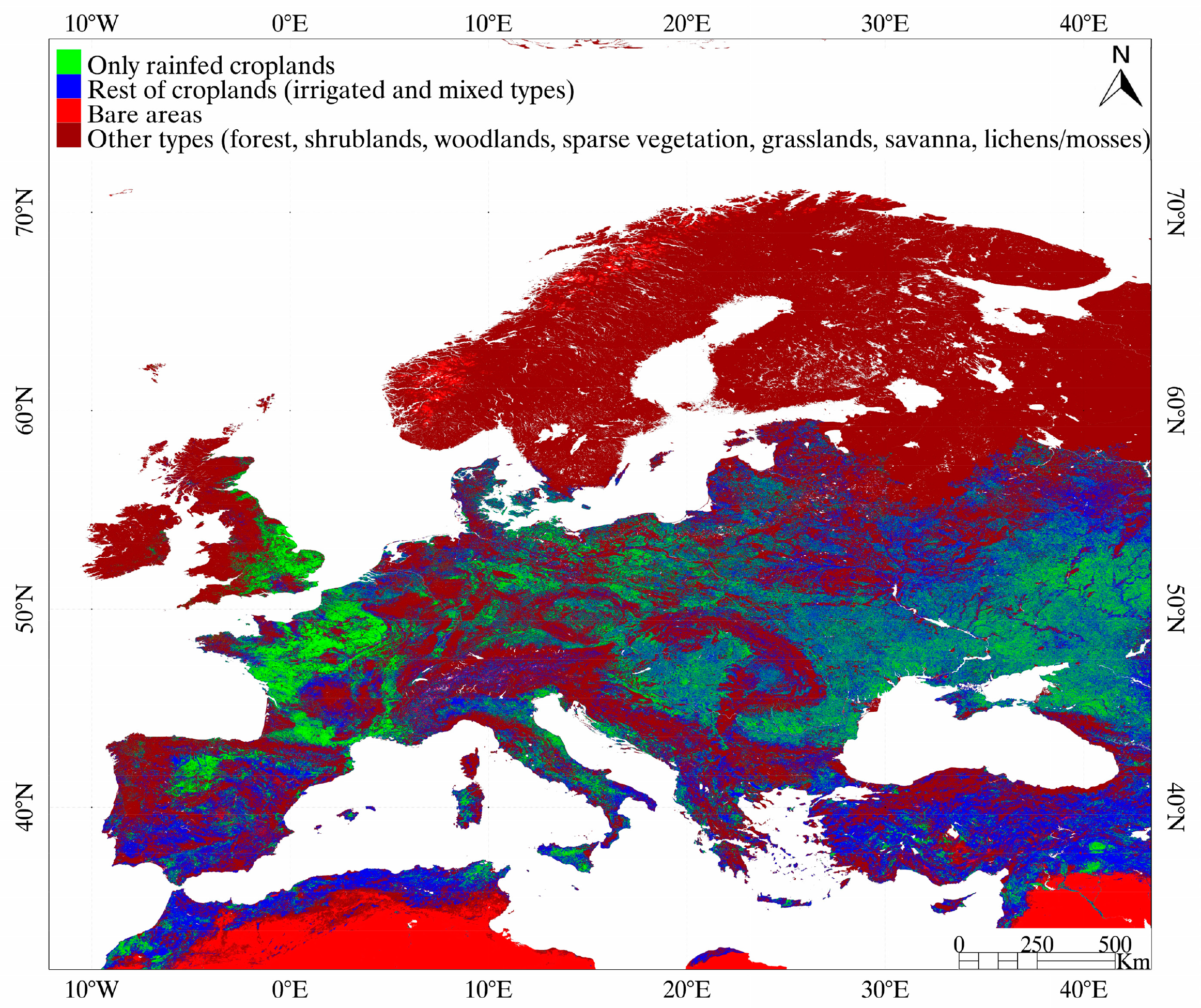
The GlobCover land cover map (ver. 2.3) [29] was used to identify the land cover type, e.g., rain–fed croplands (where the bias was calculated) and bare areas (where ETactual rates are low) (see Figure 1). More detailed information about these datasets can be found in Romaguera et al. [8].
In the research presented, daily MSG–ET values were obtained by temporal integration of the 48 instantaneous values per day, during the year 2010. Linear interpolation in time was used to fill in missing data, due to non–acquisitions. Daily MSG–ET were not considered if missing data occurred during periods of one hour or longer. Daily GLDAS–ET values were obtained by temporal averaging of the eight provided ETactual rates per day. No missing data were found in this dataset.
3.2. Data for the Classification
As explained in previous sections, four parameters were selected for the classification of the study area: (a) NDVImax; (b) a climate indicator (CI) based on net radiation, latent heat of vaporization and precipitation; (c) the maximum value of monthly aggregated ET (ETmmax); and (d) the month where the ETmmax occurs (t_ETmmax). The selected study area was Europe and the year was 2010. Additionally, the classification was also obtained in Africa for testing the method.
In order to ensure consistency of the data, the NDVImax was extracted from the source related to MSG–ET retrieval. That is the ECOCLIMAP database [30], which includes the LAI values that are used in the MSG–ET algorithm. These values are obtained by taking in situ maximum and minimum values of LAI and considering Advanced Very High Resolution Radiometer (AVHRR) NDVI series to impose seasonality per class cover. For Europe, the monthly NDVI values generated during the year 1997, by the Deutsches Zentrum für Luft– und Raumfahrt (DLR) [31], are considered, and, for Africa the International Geosphere–Biosphere Programme Data (IGBP) 1 km AVHRR NDVI composites from April 1992 until March 1993 [32]. Although these values may not represent irrigated vegetation in the year of analysis, they influence the MSG–ET retrieval and therefore the difference with GLDAS–ET, which is the focus of this research.
CI was calculated for the year 2010, according to Equation (2), by yearly aggregating Rn and P. Net radiation was obtained as the sum of net shortwave (Sn) and net longwave (Ln) radiation, which were obtained from the GLDAS dataset, together with the precipitation values.
GLDAS–ET values were aggregated monthly and the maximum value was obtained (ETmmax), as well as the month when it occurred (t_ETmmax). Radiation and ETactual values in GLDAS were given as rates every 3 h, so the proper way to calculate the yearly/monthly values was by temporal averaging of the data corrected by the time conversion factor.
The data sets were filtered according to the following criteria. Firstly, bare pixels defined by the GlobCover classification map were masked. These are arid areas, where the estimation of t_ETmmax may be affected by fluctuations of the low values of ETactual. Secondly, coastal pixels with nonrealistic values were also masked. This effect appeared when resampling the data to a common grid and pixel size. Finally, pixels with negative NDVImax value were also masked for the calculations. These were found in the datasets in areas close to water bodies. Figure 2 shows the selected data sets for the classification and the study area. Finally, every dataset was normalized dividing by its maximum and the generated four–layer file was used for the classifications.
3.3. Data for the Test of the Method
The global blue water footprint (WFb) of crop production estimated by Mekonnen and Hoekstra [3] was used to compare the ETb outputs produced in Europe and Africa. The water footprint (WF) is defined as the water consumed for crop production, where green and blue stand for precipitation and irrigation water usage. In their method, the computations of crop evapotranspiration were done following Allen et al. [33] for the case of crop growth under non–optimal conditions. The model takes into account the daily soil water balance and climatic conditions for each grid cell. Climatic and reference evapotranspiration inputs are averaged for the period 1996–2005 and results are given as average over that time interval. WFs are typically given in units of m3/ton or mm/year. In the last case, the yield is not considered and therefore WFb corresponds to total ETb. This product has global coverage and a spatial resolution of 5 arcmin.
4. Results
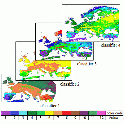
This section shows the classification maps generated with the three selected methods. The k–means and EM classifiers have a straightforward application. For the PC approach, the relationship between the first and third PC allowed identifying 11 vertical clusters, whose pixels were assigned to 11 classes (named from 1 to 11, from left to right of the Figure 3). Neither clear relationships nor groupings could be established between the PC1 and the components PC2 and PC4.
4.1. Classification Maps
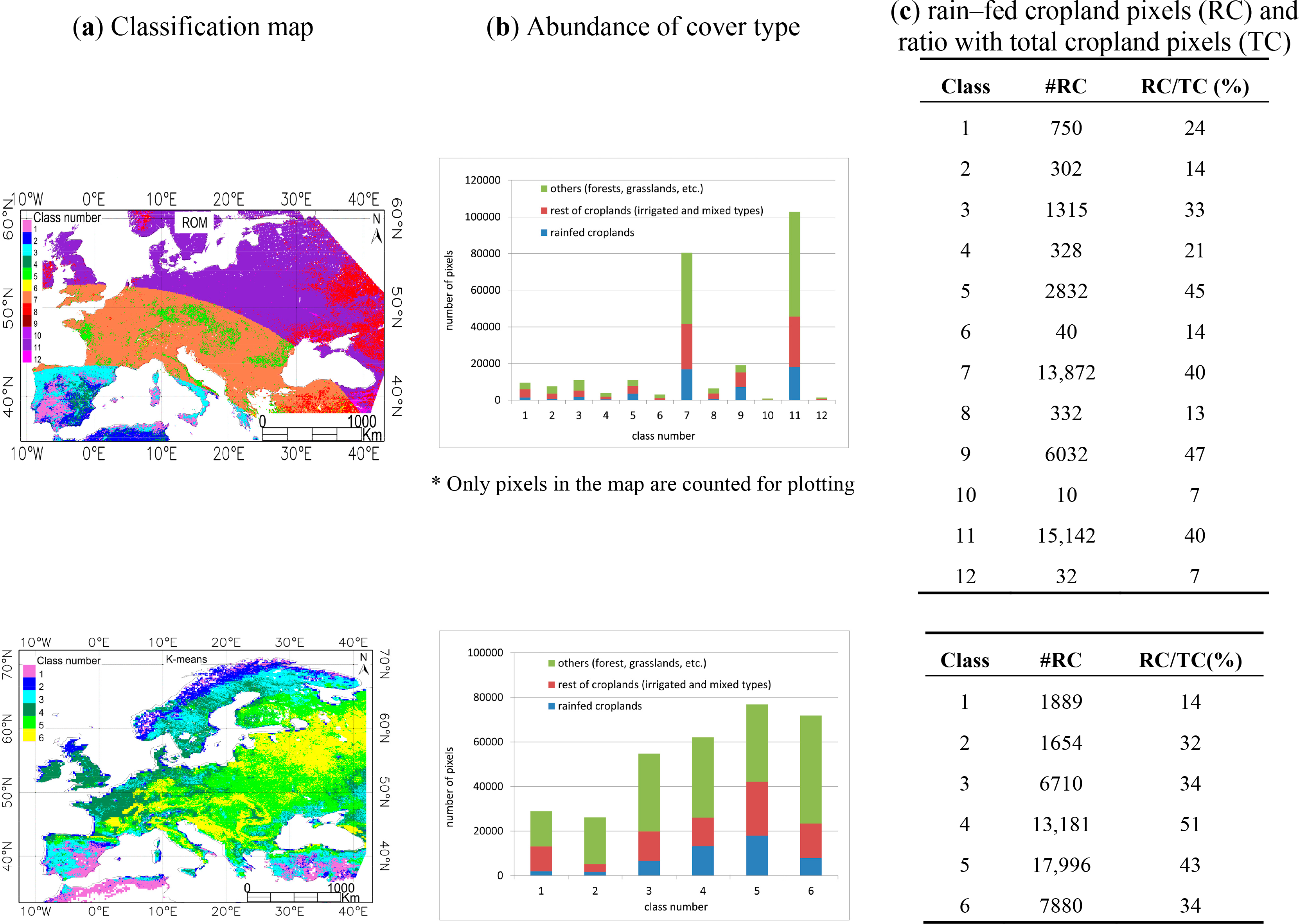
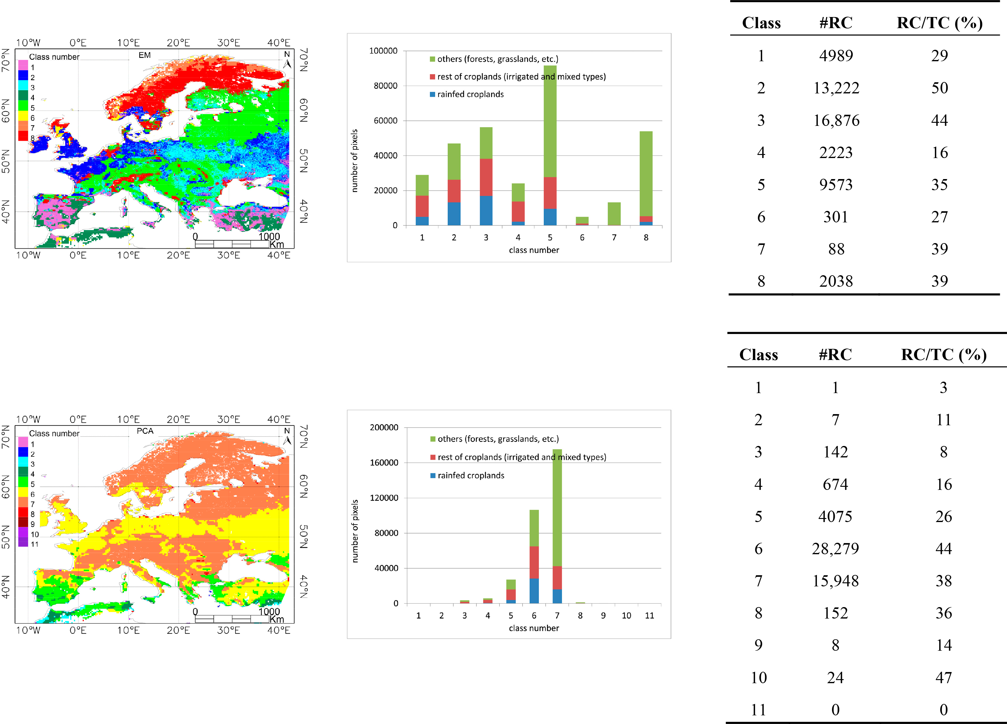
Figure 4 shows the classification maps obtained using the new set of input parameters and the three classifiers in the region of Europe. The map generated in Romaguera et al. [8] (ROM in the following) is also included for the sake of comparison. Information about the abundance of different cover types is shown per class. Three cover types are considered: (i) only rain–fed croplands; (ii) rest of croplands (irrigated and mixed types); and (iii) others (forests, shrublands, woodlands, sparse vegetation, grassland, savanna, lichens/mosses), according to the GlobCover map. Additionally, the number of rain–fed croplands (RC) and the ratio of these over the total croplands (RC/TC) are incorporated.
The number of classes generated was 12, 6, 8, and 11 in the ROM, k–means, EM and PCA classifications respectively. The numbers assigned to the classes must be understood as labels and their value is not necessarily related between the different classification outputs. In general, the proposed classifications had a visually more continuous spatial distribution than ROM, which presented the characteristic rings due to the intervals chosen in the VZA criteria. Moreover, some similar grouping can be observed in the generated classifications, such as the areas of Spain and East and center Europe in EM and PCA or Eastern part of Norway in k–means and EM, although this comparison is not easy to evaluate. The distribution of the classes in the k–means and EM classification showed the influence of all four input parameters, whereas in the PCA classification output, the parameter determining the classes was the t_ETmmax. This is associated to the fact that the third component of the PCA captures the variability (after transformation) of the discrete values of t_ETmmax.
Two majority classes were found in the ROM classification, as well as in PCA. That is represented in Figure 4b by the total height of the columns. However, the abundance of the classes in k–means and EM was more balanced, with no significant minority classes in the case of k–means.
The blue color in the graphs indicates the amount of rain–fed croplands per class, which is also indicated in Figure 4c. This number is important since the bias is calculated in this cover type. Therefore in classes 6, 10, 12 from ROM and classes 1, 2, 9, and 10 from PCA, the bias was calculated with relatively few samples. Additionally, class 11 in PCA had no rain–fed pixels and the bias could not be calculated.
Another relevant factor is the relative abundance of rain–fed croplands with respect to the total number of croplands (rain–fed plus rest of croplands) per class. The ETb is ultimately calculated in all croplands, and therefore this ratio (named RC/TC in the following) is important. The higher RC/TC is, the more representative the bias is for all the pixels in a class, that is in classes 3, 5, 7, 9, 11 from ROM, 2 until 6 in k–means, 2, 3, 5, 7, 8 in EM, and 6, 7, 8, 10 in PCA. These classes had a ratio higher than 30%, as can be observed in Figure 4c.
As a result of this analysis, it was concluded that the k–means and EM classification schemes improved the existing one (ROM) in two aspects: the spatial pattern of the classification map and the increase in number of rain–fed pixels and RC/TC per class, with less minority classes, showing the k–means a better performance. The PCA approach showed weaker changes.
The evaluation of the performance of the classifications is detailed in the Discussion section.
4.2. Bias Curves
The bias values were obtained per pixel at monthly scale. Monthly ETactual values were obtained from the daily MSG–ET and GLDAS–ET estimates during 2010. Due to the lack of some MSG–ET data, and in order to obtain a consistent bias curve, the daily values were only aggregated when both datasets existed. Then, monthly bias values were obtained per pixel and yearly curves were averaged per class, using rain–fed pixels only, for each of the classifications.
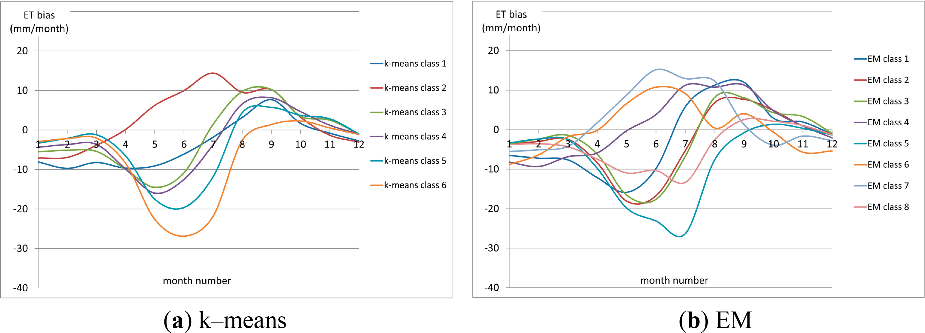
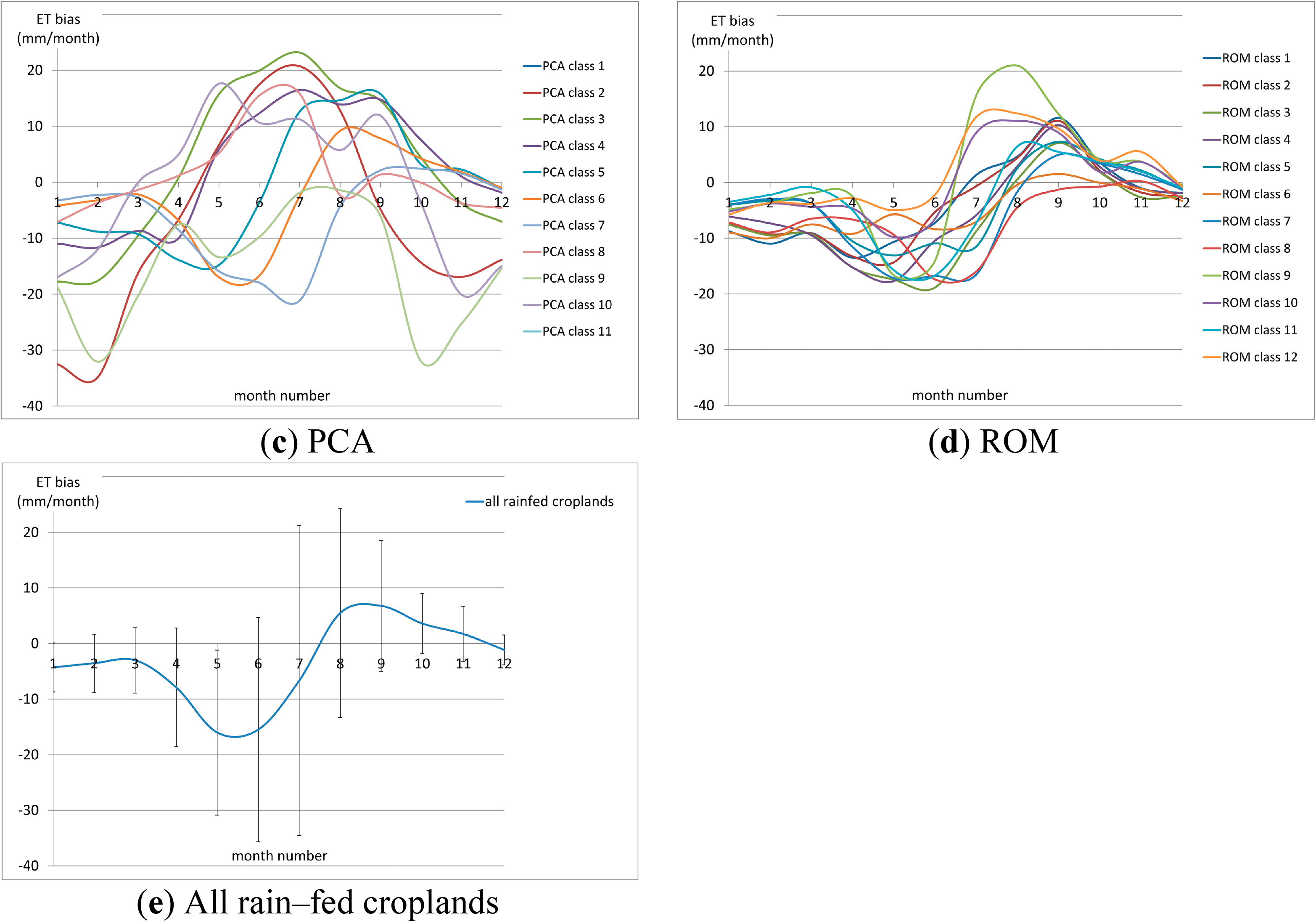
Figure 5 shows the bias curves using the three proposed classifiers and ROM. Additionally the mean bias curve using all rain–fed croplands is plotted as a reference. Note that they are discrete monthly values that are connected to facilitate visual interpretation.
In general it was observed that the k–means and EM classifications achieved a better separation of the bias curves, compared with ROM and PCA. The k–means curves (Figure 4a) presented a minimum around the month of June in classes 3, 4, 5, and 6 with a general convex shape and amplitude up to −28 mm/month. A local maximum was found around August. The curves of classes 1 and 2 were concave and corresponded to classes with relatively low number of rain–fed croplands, achieving for class 1 the lowest RC/TC ratio (see Figure 4c).
Classes 1, 2, 3, 5, and 8 in EM also presented a convex bias with maximum amplitude around May–June with values up to −28 mm/month. A local maximum was found around August. Classes 4, 6 and 7 were concave; 4 and 6 corresponded to lowest ratio RC/TC and class 7 to lowest value of rain–fed croplands.
In the PCA classification, classes 5, 6, and 7 behaved in a similar way as the convex curves described for k–means and EM. These were the classes with higher number of rain–fed pixels and also high RC/TC. Classes 2, 3, 4, 8 and 10 were concave and presented more irregular bias curves. These were less abundant classes, some of them not even noticeable visually in the figure, in general they had lower ratio RC/TC and relatively low number of pixels. Class number 9 presented an intermediate pattern and classes 1 and 11 were not plotted since they contained only one rain–fed pixel or none.
The biases obtained from the ROM classification were more fuzzy and irregular. Some of the classes (3, 5, 7, 8, 9, and 11) presented a convex shape similar to the aforementioned curves, but the pattern was irregular and it was difficult to distinguish between classes and extract conclusions regarding the amount of rain–fed croplands and RC/TC.
Finally, Figure 5e shows the variability of the bias curve when all rain–fed croplands are averaged and no classes are taken into account. The position of the minimum and local maxima is consistent with what it has been described in this paper, and the amplitude is in general flattened due to the averaging.
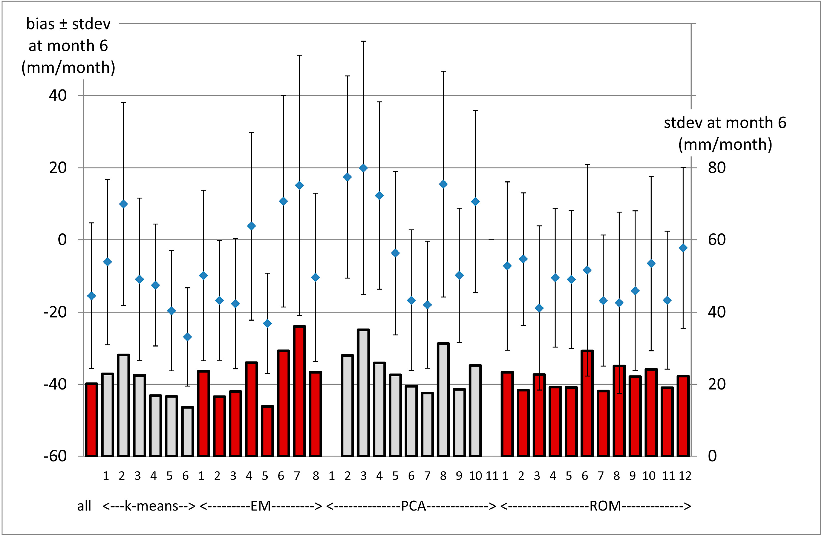
In general the k–means and EM approach represented an improvement with respect to the ROM bias results in terms of separation of the bias curves, which means a better discrimination of the classes. Furthermore, differences in the maximum amplitude of the curves were also found. In order to understand them better, Figure 6 shows the comparison of the bias values around the maximum (month six) (represented as dots) together with the standard deviation associated to it (represented as error bars and also in columns). This was obtained for all the classes and for the mean curve where no classes are assigned (Figure 5e).
Figure 6 shows how the standard deviation (σ, in columns and secondary Y axis) changed when adding a classification in the method instead of using a single bias curve averaged for all rain–fed croplands. In general, the diminution of σ was found in majority classes. In the case of the k–means classifier, σ was reduced in classes 4, 5, and 6 and slightly increased in classes 1, 2, and 3. For the EM classifier, σ increased in classes 1, 4, 6, 7, and 8. In general terms, σ increased in the PCA classification, and the values in ROM fluctuated depending on the class. It was also observed that the increase of σ was related with the decrease of number of rain–fed croplands and RC/TC in the class.
In terms of the bias value, the classifiers captured different intervals of variability: between −27 and 10 mm/month in k–means, between −23 and 15 mm/month for EM, between −18 and 20 mm/month for PCA and between −19 and −2 mm/month for ROM. The value of the bias for the single curve was −15 mm/month. Therefore the proposed classifiers captured a higher range of bias with respect to ROM.
Previous literature showed the differences between MSG–ET and GLDAS–ET [13,34]. For the region of Europe, these studies showed the bias relative to the mean MSG–ET, with values ranging from −0.5 to 0.5. The mean MSG–ET in the month of July was also plotted in this literature, with a value of 0.22 mm/h calculated in the range 9–12UTC. If we assume a constant ETactual rate, and 10 h of sun, the aggregated value is 66 mm/month. This value combined with the ±0.5 values of relative bias, produces values of absolute bias up to 33 mm, which is consistent with the intervals found with the proposed classifiers.
As a result of this analysis, the k–means approach showed to improve the existing methodology and perform better than EM and PCA in different aspects related with the bias estimation; first, the ability to differentiate bias curves; second, by reducing the standard deviation of the data when introducing the classes; third, by capturing the expected variability of the maximum bias.
Therefore based on the conclusions extracted from the classification and bias analysis, the k–means is used in the following to estimate ETb, since it was shown to be the most suitable approach for this research.
4.3. ETb Estimation
ETb was obtained in the region of Europe in 2010 following Equation (1), the k–means classification and the bias results. ΔET values were calculated daily when both datasets were available and then accumulated monthly. Monthly bias corrections were undertaken, and the resulting positive ETb values were aggregated to a yearly scale.
According to the method described in Romaguera et al. [8], the GlobCover map was used to mask all cover types except for the rain–fed croplands, irrigated croplands and mixed types that include croplands. Although in that publication a value of 50 mm was suggested as a threshold from which the method was able to detect irrigation, in the current research, no threshold was considered based on the fact that small values of ETb may be also representative for heterogeneous pixels.
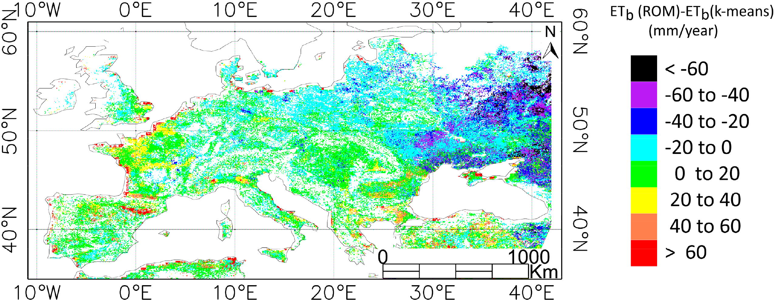
The same procedure was used to obtain ETb using the classification scheme provided in the literature (ROM). The comparison showed how the outputs changed when using a different classification scheme. ETb reached differences up to 60 mm/year, being ETb (k–means) higher in some regions of Ukraine and lower in some regions of Spain, Turkey and coast of France. The spatial distribution of these differences is related with the classification maps, being for example the red areas in Figure 7 associated with class number 2 of the k–means classification that has a convex shaped bias.
5. Application of the Method
The study area selected to test the method was the whole Meteosat observation disk, which included Europe and Africa, in the year 2010. The analysis was carried out by separating it in three sectors namely Europe, North Africa, and South Africa, like the MSG–ET products delivered by LSA–SAF. These sections are separated at the latitudes of 34°N and the equator approximately.
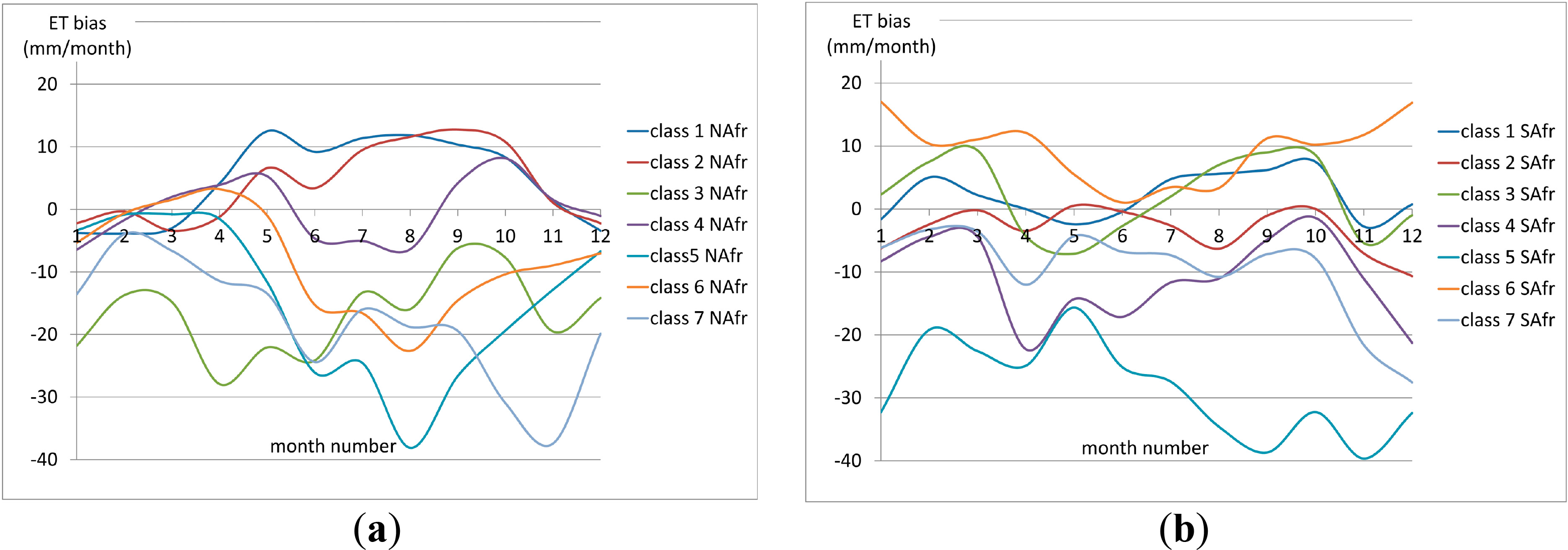
Following the method explained in the present paper, a classification of every sector was carried out with the k–means algorithm using the proposed input data sets. Pixels labeled as bare areas by the GlobCover map were excluded from the classification. The optimal number of classes was calculated per sector following the procedure explained in Section 2.2.1. The bias curves per class in the rain–fed pixels of North Africa and South Africa are plotted in Figure 8.
Similarly to the conclusions found in Europe using the k–means approach (Figure 5), the curves present distinguishable patters with different amplitudes and shapes. Classes 1, 4 and 6 in North Africa present more defined convex bias curves which correspond to highest numbers of rain–fed pixels and ratio RC/TC, whereas classes 3 and 7 are represented by the lowest number of rain–fed pixels and ratio RC/RT. In the sector of South Africa, the curves present a shift of about six months with respect to the sectors of Europe and North Africa. This is due to the seasonality patterns of the southern Hemisphere. The most abundant classes in terms of rain–fed pixels were classes 2, 4, and 7. However, due to the relatively low quantity of rain–fed pixels in this sector, the ratio RC/TC is below 10% for all the classes in South Africa.
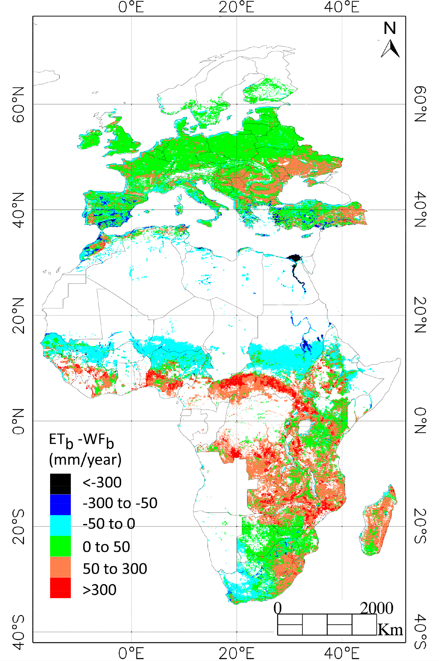
Equation (1) was used in all the study area to calculate monthly ETb and the positive values were aggregated to a yearly scale. These were compared with the values of blue water footprint (WFb) for crop production estimated by Mekonnen and Hoekstra [3]. For consistency, the areas labeled with no irrigation croplands in Mekonnen and Hoekstra [3] were masked (see Figure 9).
The mean value of the differences found in Europe and Africa was 27 and 62 mm/year with standard deviation of 62 and 142 mm/year, and rmse of 44 and 155 mm/year. No straightforward correlation was found between the two datasets. Differences between the two methods were found to be below 50 mm/year in most of Europe and in some regions of Africa, although in this area the discrepancies (in positive and negative sign) were higher as also shown by the statistical indicators. Several reasons exist to explain the magnitude and sign of the differences.
First, from a methodological point of view, Mekonnen and Hoekstra [3] used the cropmap of Monfreda et al. [35] to correct the calculated ETactual with the percentage of cropland per pixel, and then the irrigated area map from Portmann et al. [36] to correct for the area used for irrigation. This resulted in values of annual ETb lower than the ones generated in this paper, as it can be observed in most of Europe and some regions in Africa indicated with green color.
Higher discrepancies (in orange and red) were found in mid Africa. This can be explained based on the cover type and pixel heterogeneity, since these are areas labeled as forests and shrublands by the GlobCover map. The method by Mekonnen and Hoekstra [3] provided low values of ETb (below 1 mm/year) in these mixed pixels due to low value of irrigated cropland area. However, the method presented in this paper and the bias estimation were not developed for cover types different than croplands, and therefore the values obtained in these areas are not realistic and should be masked as indicated by Romaguera et al. [8]. This is the case also of the forested areas in Spain, Italy, Greece, and Turkey.
The region of Ukraine presented higher values of ETb compared with the estimates given by Mekonnen and Hoekstra [3]. This can be explained by a combination of factors. Low values of ETb were obtained by Mekonnen and Hoektra [3] in the majority of this area. Higher values were obtained by the proposed method, which were influenced by the high values of ΔET found in the inputs. Moreover, this region is located in the extremes of the Meteosat observation disk, which might influence the accuracy of the remote sensed ETactual estimates.
Areas painted in cyan were labeled as bare areas by the GlobCover map and were masked in the classification carried out in the present paper. That was done to avoid misclassification caused by the fluctuation of low ETactual rates in these areas. Therefore, the method did not provide ETb values, whereas Mekonnen and Hoekstra [3] estimated values of ETb below 1 mm/year. Moreover, other bare areas were also masked in the present paper and they provided significantly high values of ETb in the estimates of the literature. That was the case of the White Nile in Sudan and some areas in Morocco.
Mekonnen and Hoekstra [3] provided significantly higher values of ETb in the region of the Nile basin. These are areas where the assigned cropland irrigated area from Portmann et al. [36] was higher than 100%, a fact that was related to multiple cropping practices. ETb estimates were higher than 1000 mm/year in this case. However, the method presented in this paper relied only on the differences between the ETactual inputs from MSG and GLDAS and the bias correction, achieving annual values in this region of 600 mm/year.
Moreover, the discrepancies in some mountainous areas like Mozambique, Ethiopia or north of Italy, may be associated to the effect of the terrain on the radiation. In zones of complex topography, variability in elevation, surface slope and aspect create strong spatial heterogeneity in solar distribution, which determines air temperature, soil temperature, ET, snow melt and land–air exchanges. Therefore, MSG–ET satellite retrievals may need a slope and aspect correction to radiation inputs in areas of significant relief. Some remote sensing methods that include this geometric correction for calculating ET are given by Allen et al. [37] and Chen et al. [38]. Finally, together with the aforementioned methodological reasons, the differences between the two estimates might be related to the accuracy and parameterization of the input data, and the period of comparison, since the datasets were obtained at different time spans.
6. Discussion
6.1. Uncertainty
6.1.1. Performance of the Classifications
Evaluating the performance of the generated classifications is not an easy task, especially due to the fact that a “ground truth classification map” that explains the different classes in terms of the biases between MSG–ET and GLDAS–ET does not exist. However, in order to optimize the performance of the methods, different strategies were adopted. The k–means settings were adjusted to a maximum of 100 iterations in order to ensure completion of the algorithm and the optimal number of clusters was calculated using a quality index [23] that accounts for the intra–cluster and inter–cluster distances, as it is shown in Section 1.2.1.
The EM algorithm was trained with 66% of the data, and tested in the rest of the dataset providing a log likelihood of 7.04 in the test. The overall likelihood is a measure of the “goodness” of the clustering and increases at each iteration of the EM algorithm. The larger this quantity is, the better the model fits the data. In order to interpret this number, the model was applied to the whole dataset, obtaining a log likelihood of 7.6. This value was expected to be higher than using only the test dataset since the inputs included also the training data. However, the two log likelihood values were similar, which served as an indicator of the good performance of the classifier. Moreover, the EM algorithm found the optimal number of clusters for which the log likelihood had a maximum value.
Finally the PC analysis was carried out by using two matrixes, the covariance and the correlation matrixes. The results showed the same clustering using both procedures, where the groups could be visually identified as it is shown in Figure 3. The usefulness of the generated classifications in the application that is presented in this paper (bias estimation and ETb), was discussed in Section 4.2.
6.1.2. Uncertainty of ETb Estimations
It was pointed out in Romaguera et al. [8] that Equation (1) provided some negative values of ETb which were not physically correct and were due to the uncertainties in the input data and in the bias curves definition. In the present work, these negative values were not used in the calculation of the annual ETb and in order to evaluate their significance they were aggregated during 2010 and combined with the yearly MSG–ET. The ratio between these two (not shown here) was less than 10% in most of the croplands in the study area. The impact of the negative values was concentrated in areas labeled as “others” (see Figure 1) or in their proximity, like next to the Alps and the Carpathian mountains.
Therefore, it was shown that with the proposed method the non–croplands pixels are more sensitive to errors and, therefore, they should be masked when producing ETb.
6.2. Limitations
This paper focused on the improvement of the classification scheme proposed by Romaguera et al. [8]. The analysis presented showed satisfactory results when producing the classification maps and obtaining the bias curves. General limitations and aspects to be taken into consideration when obtaining ETb are extensively discussed in the aforementioned literature, and are related to the inaccuracies of the inputs, data availability, validation drawbacks and generalization of the method.
Regarding the classification approach presented in this paper, several aspects need to be discussed.
First, the selection of the parameters for the classification is justified in the text. However, additional parameters may have been used and a sensitivity analysis might be carried out to select the optimal set to describe the study area.
Regarding the selection of the classifier, this work showed three strategies, different in concept and complexity. The k–means showed to work better in this research. Nevertheless, having in mind the coarse resolution of the data used, subpixel classifiers may be explored in order to account for mixed pixels and subpixel heterogeneity. In that case, aspects like avoiding over classification and tradeoffs in accuracy, time consumption and computing resources would need to be taken into account. Also, the better performance of the k–means approach, as compared to EM and PCA, was not tested in the application for Africa.
The dimensions of the study area may play an important role when the classifier finds similar pixels apart of each other (e.g., North and South Africa). The bias value may be influenced by the averaging of rain–fed areas in these distant areas. Therefore, a preliminary test on qualitative differences in sub–continental bias patterns is advised to avoid these effects and select reasonable study area sizes.
The GlobCover land cover map was used in several steps in this paper, to mask bare areas in the classification, to identify rain–fed croplands where the bias curves were obtained and finally to filter other land covers for ETb estimation. The results are therefore influenced by the inaccuracies of this input, since pixels may be misclassified.
From a technical point of view, the rescaling and resampling of the input data to achieve a common spatial resolution may have an impact in the analysis. The nearest neighbor resampling technique was used in this research. In general, impacts on the results are expected due to the heterogeneity of the surface and the question of how representative are the low resolution data disaggregated to a higher scale. Up–downscaling techniques tackle this issue by using the parameters of surface temperature or NDVI [39,40].
The ETb results compared with existing literature provided differences of 50 mm/year in most of Europe. In Africa, the comparison was highly influenced by the assigned cover type and the heterogeneity of the pixel. Results over regions of high topographic relief point to the need for slope and aspect corrections to radiation inputs to the MSG–ET algorithm. Bearing in mind the advantages of both approaches (literature and present paper), the synergy between them may allow to benefit from the temporal frequency of the remote sensed data and from the better definition of the subpixel heterogeneity.
The in situ validation of the ETb estimates produced in this paper is hampered by the scarcity of good quality spatial data on irrigation at regional scale. The availability of irrigation water management information on a detailed scale like farmer fields or for entire river basins is not common. Data to quantify performance indicators are rarely collected. If collected, data frequently is unreliable or not easily accessible [10]. An attempt was made in previous literature to validate the methodology in a corn field in a cropland area in Spain [8]. Difficulties were found due to the unavailability of MSG–ET remote sensing data coincident with the literature, together with the fact that water resources and irrigation are politically critical issues and generally practices are not regulated or in situ quality data are difficult to access. Moreover, statistical databases such as AQUASTAT [41] provide static and scattered data. Therefore, the validation of the improved method with in situ data remains an open challenge. Although further research is needed to fully understand the ETb values found, this paper has shown to improve the classification scheme and the estimation of the bias curves between the sets of ET data from MSG and GLDAS. An example of application of this improved method to time series of data in the Horn of Africa and Southwest of China is presented in Romaguera et al. [42].
7. Conclusions
This paper provided a more generic and robust methodology to estimate blue water evapotranspiration (ETb) from remote sensing and simulated ETactual data, by enhancing the classification scheme employed in the literature. A new selection of input parameters was proposed and the analysis of different classifiers provided the best results for the k–means technique.
The main outcome was the improvement of the definition of the bias between the two ETactual datasets, i.e., the ability to differentiate bias curves of different classes, reduction of the standard deviation of the data and achievement of the expected variability of the maximum bias.
This paper proposed new tools to evaluate the variability of the biases between remote sensing and simulated ETactual data. However, the comparison of ETb in Europe and Africa with existing literature showed the need of further research to fully understand the final ETb values found.
Acknowledgments
The authors wish to thank the Land Surface Analysis Satellite Applications Facility (LSA–SAF) of the European Organisation for the Exploitation of Meteorological Satellites (EUMETSAT), as well as the European Space Agency (ESA) and the ESA GlobCover Project, led by MEDIAS–France, for providing the products used in this paper. The GLDAS data used in this study were acquired as part of the mission of NASA’s Earth Science Division and archived and distributed by the Goddard Earth Sciences (GES) Data and Information Services Center (DISC).
Author Contributions
This work was carried out in the framework of the PhD research of the first author M. Romaguera. The coauthors have contributed as supervisors of this project.
Conflicts of Interest
The authors declare no conflict of interest.
References
- Hanasaki, N.; Inuzuka, T.; Kanae, S.; Oki, T. An estimation of global virtual water flow and sources of water withdrawal for major crops and livestock products using a global hydrological model. J. Hydrol 2010, 384, 232–244. [Google Scholar]
- Liu, J.G.; Yang, H. Spatially explicit assessment of global consumptive water uses in cropland: Green and blue water. J. Hydrol 2010, 384, 187–197. [Google Scholar]
- Mekonnen, M.M.; Hoekstra, A.Y. The green, blue and grey water footprint of crops and derived crop products. Hydrol. Earth Syst. Sci 2011, 15, 1577–1600. [Google Scholar]
- Siebert, S.; Döll, P. Quantifying blue and green virtual water contents in global crop production as well as potential production losses without irrigation. J. Hydrol 2010, 384, 198–217. [Google Scholar]
- Siebert, S.; Döll, P.; Hoogeveen, J.; Faures, J.M.; Frenken, K.; Feick, S. Development and validation of the Global Map of Irrigation Areas. Hydrol. Earth Syst. Sci 2005, 9, 535–547. [Google Scholar]
- Thenkabail, P.S.; Biradar, C.M.; Noojipady, P.; Dheeravath, V.; Li, Y.J.; Velpuri, M.; Gumma, M.; Gangalakunta, O.R.P.; Turral, H.; Cai, X.L.; et al. Global Irrigated Area Map (GIAM), derived from remote sensing, for the end of the last millennium. Int. J. Remote Sens 2009, 30, 3679–3733. [Google Scholar]
- Romaguera, M.; Hoekstra, A.Y.; Su, Z.; Krol, M.S.; Salama, M.S. Potential of using remote sensing techniques for global assessment of water footprint of crops. Remote Sens 2010, 2, 1177–1196. [Google Scholar]
- Romaguera, M.; Krol, M.S.; Salama, M.S.; Hoekstra, A.Y.; Su, Z. Determining irrigated areas and quantifying blue water use in Europe using remote sensing Meteosat Second Generation (MSG) products and Global Land Data Assimilation System (GLDAS) data. Photogramm. Eng. Remote Sens 2012, 78, 861–873. [Google Scholar]
- Romaguera, M.; Salama, M.S.; Krol, M.S.; Su, Z.; Hoekstra, A.Y. Remote sensing method for estimating green and blue water footprint. In Remote Sensing and Hydrology; Neale, C.M.U., Cosh, M.H., Eds.; The International Association of Hydrological Sciences: Wallingford, UK, 2012; Volume 352, pp. 288–291. [Google Scholar]
- Bastiaanssen, W.G.M.; Bos, M.G. Irrigation performance indicators based on remotely sensed data: A review of literature. Irrig. Drain. Syst 1999, 13, 192–311. [Google Scholar]
- Santos, C.; Lorite, I.J.; Tasumi, M.; Allen, R.G.; Fereres, E. Performance assessment of an irrigation scheme using indicators determined with remote sensing techniques. Irrig. Sci 2010, 28, 461–477. [Google Scholar]
- D’Urso, G.; de Michele, C.; Vuolo, F. Operational irrigation services from remote sensing: The irrigation advisory plan for the Campania region, Italy. In Remote Sensing and Hydrology; Neale, C.M.U., Cosh, M.H., Eds.; The International Association of Hydrological Sciences: Wallingford, UK, 2012; Volume 352, pp. 419–422. [Google Scholar]
- Ghilain, N.; Arboleda, A.; Gellens–Meulenberghs, F. Evapotranspiration modelling at large scale using near–real time MSG SEVIRI derived data. Hydrol. Earth Syst. Sci 2011, 15, 771–786. [Google Scholar]
- Rodell, M.; Houser, P.R.; Jambor, U.; Gottschalck, J.; Mitchell, K.; Meng, C.J.; Arsenault, K.; Cosgrove, B.; Radakovich, J.; Bosilovich, M.; et al. The Global Land Data Assimilation System. Bull. Am. Meteorol. Soc 2004, 85, 381–394. [Google Scholar]
- Romaguera, M.; Salama, S.; Krol, M.S.; Hoekstra, A.Y.; Su, Z. Synergy between remote sensing ET products and simulated data to retrieve irrigated areas and blue ET in Europe and Africa. Poster. Presented at the 5th International Workshop on Catchment Hydrological Modeling and Data Assimilation CAHMDA–V: Catchments in a Changing Climate, Enschede, The Netherlands, 9–13 July 2012; p. 1.
- LSA–SAF. LSA–SAF Validation Report. Products LSA–16 (MET), LSA–17 (DMET); Doc. Num. SAF/LAND/RMI/VR/0.6; The EUMETSAT; Network of Satellite Application Facilities: Darmstadt, Germany, 2010. [Google Scholar]
- Yilmaz, M.T.; Anderson, M.C.; Zaitchik, B.; Hain, C.R.; Crow, W.T.; Ozdogan, M.; Chun, J.A.; Evans, J. Comparison of prognostic and diagnostic surface flux modeling approaches over the Nile river basin. Water Resour. Res 2014, 50, 386–408. [Google Scholar]
- Roerink, G.J.; Menenti, M.; Soepboer, W.; Su, Z. Assessment of climate impact on vegetation dynamics by using remote sensing. Phys. Chem. Earth 2003, 28, 103–109. [Google Scholar]
- Price, K.P.; Guo, X.L.; Stiles, J.M. Optimal Landsat TM band combinations and vegetation indices for discrimination of six grassland types in eastern Kansas. Int. J. Remote Sens 2002, 23, 5031–5042. [Google Scholar]
- Lu, D.; Weng, Q. A survey of image classification methods and techniques for improving classification performance. Int. J. Remote Sens 2007, 28, 823–870. [Google Scholar]
- Tou, J.T.; Gonzalez, R.C. Pattern Recognition Principles; Addison–Wesley Publishing Company: Reading, MA, USA, 1974. [Google Scholar]
- Exelis Visual Information Solutions. ENVI Tutorial: Classification Methods; Exelis Visual Information Solutions: Boulder, CO, USA, 2006. [Google Scholar]
- Rezaee, M.R.; Lelieveldt, B.P.F.; Reiber, J.H.C. A new cluster validity index for the fuzzy c–mean. Pattern Recognit. Lett 1998, 19, 237–246. [Google Scholar]
- Dempster, A.P.; Laird, N.M.; Rubin, D.B. Maximum likelihood from incomplete data via the EM algorithm. J. R. Stat. Soc. B 1977, 39, 1–38. [Google Scholar]
- Hall, M.; Frank, E.; Holmes, G.; Pfahringer, B.; Reutemann, P.; Witten, I.H. The WEKA data mining software: An update. Sigkdd Explor 2009, 11, 10–18. [Google Scholar]
- Richards, J.A.; Jia, X. Remote Sensing Digital Image Analysis: An Introduction; Springer–Verlag: Berlin, Germany, 1999; p. 240. [Google Scholar]
- Chen, F.; Mitchell, K.; Schaake, J.; Xue, Y.K.; Pan, H.L.; Koren, V.; Duan, Q.Y.; Ek, M.; Betts, A. Modeling of land surface evaporation by four schemes and comparison with FIFE observations. J. Geophys. Res.: Atmos 1996, 101, 7251–7268. [Google Scholar]
- Koren, V.; Schaake, J.; Mitchell, K.; Duan, Q.Y.; Chen, F.; Baker, J.M. A parameterization of snowpack and frozen ground intended for NCEP weather and climate models. J. Geophys. Res.: Atmos 1999, 104, 19569–19585. [Google Scholar]
- UCLouvain/ESA. Globcover 2009. Products Description and Validation Report; European Space Agency; Paris, France, 2011. [Google Scholar]
- Masson, V.; Champeaux, J.L.; Chauvin, F.; Meriguet, C.; Lacaze, R. A global database of land surface parameters at 1–km resolution in meteorological and climate models. J. Clim 2003, 16, 1261–1282. [Google Scholar]
- Mucher, C.A.; Champeaux, J.L.; Steinnocher, K.T.; Griguolo, S.; Wester, K.; Heunks, C.; Winiwater, W.; Kressler, F.P.; Goutorbe, J.P.; ten Brink, B.; et al. Development of a Consistent Methodology to Derive Land Cover Information on an European Scale from Remote Sensing for Environmental Modeling; Center for Geo–Information (CGI) Alterra: Wageningen, The Netherlands, 2001; p. 160. [Google Scholar]
- Belward, A.S.; Estes, J.E.; Kline, K.D. The IGBP/DIS global 1–km land–cover data set discover. A project overview. Photogramm. Eng. Remote Sens 1999, 65, 1013–1020. [Google Scholar]
- Allen, R.; Pereira, L.S.; Raes, D.; Smith, M. FAO Irrigation and Drainage Paper N. 56: Crop Evapotranspiration; Food and Agriculture Organization: Rome, Italy, 1998. [Google Scholar]
- Gellens–Meulenberghs, F.; Arboleda, A.; Ghilain, N. Towards a continuous monitoring of evapotranspiration based on MSG data. In IAHS Symposium on Remote Sensing for Environmental Monitoring and Change Detection; IAHS Press; Wallingford, UK, 2007. [Google Scholar]
- Monfreda, C.; Ramankutty, N.; Foley, J.A. Farming the planet: 2. Geographic distribution of crop areas, yields, physiological types, and net primary production in the year 2000. Glob. Biogeochem. Cycle 2008. [Google Scholar] [CrossRef]
- Portmann, F.T.; Siebert, S.; Döll, P. MIRCA2000–global monthly irrigated and rainfed crop areas around the year 2000: A new high–resolution data set for agricultural and hydrological modeling. Glob. Biogeochem. Cycle 2010. [Google Scholar] [CrossRef]
- Allen, R.G.; Tasumi, M.; Trezza, R. Satellite–based energy balance for mapping evapotranspiration with internalized calibration (METRIC)–model. J. Irrig. Drain. Eng 2007, 133, 380–394. [Google Scholar]
- Chen, X.; Su, Z.; Ma, Y.; Yang, K.; Wang, B. Estimation of surface energy fluxes under complex terrain of Mt. Qomolangma over the Tibetan plateau. Hydrol. Earth Syst. Sci 2013, 17, 1607–1618. [Google Scholar]
- Anderson, M.C.; Kustas, W.P.; Norman, J.M. Upscaling flux observations from local to continental scales using thermal remote sensing. Agron. J 2007. [Google Scholar] [CrossRef]
- Jia, S.; Zhu, W.; Lű, A.; Yan, T. A statistical spatial downscaling algorithm of TRMM precipitation based on NDVI and DEM in the Qaidam basin of China. Remote Sens. Environ 2011, 115, 3069–3079. [Google Scholar]
- FAO. Aquastat Database; Food and Agriculture Organization: Rome, Italy, 2009; Available online: http://www.fao.org/nr/water/aquastat/main/index.stm (accessed on 15 July 2014). [Google Scholar]
- Romaguera, M.; Krol, M.S.; Salama, S.; Su, Z.; Hoekstra, A.Y. Application of a remote sensing method for estimating monthly blue water evapotranspiration in irrigated agriculture. Remote Sens 2014. submitted.. [Google Scholar]


| Data | Source | Spatial Coverage | Spatial Resolution | Temporal Resolution | Details |
|---|---|---|---|---|---|
| ETactual | MSG | MSG disk * | 3 km at nadir | 30’ | Availability of data: Europe: January 2007–present The rest: September 2009–present |
| GLDAS | Global | 0.25° (∼30 km at equator) | 3 h | Availability of data: February 2000–present | |
| Sn, Ln, P | GLDAS | Global | 0.25° (∼30 km at equator) | 3 h | Availability of data: February 2000–present |
| Land Cover | MERIS | Global | 300 m | Static | GlobCover map calculated in year 2009 |
| NDVI | AVHRR | Europe | 1 km | Monthly | Generated by DLR Period: year 1997 |
| Africa | Generated by IGBP Period: April 1992–March 1993 | ||||
| Irrigation | Blue WF | Global | 5 arcmin (∼10 km at equator) | Static | Data: blue WF per year[3] |
*Meteosat disk covers latitudes between −60° and +60° and longitudes between −60° to +60°;**List of acronyms: MSG (Meteosat Second Generation), GLDAS (Global Land Data Assimilation System), MERIS (Medium Resolution Imaging Spectrometer), AVHRR (Advanced Very High Resolution Radiometer), DLR (Deutsches Zentrum für Luft– und Raumfahrt), IGBP (International Geosphere–Biosphere Programme Data), WF (Water Footprint).
© 2014 by the authors; licensee MDPI, Basel, Switzerland This article is an open access article distributed under the terms and conditions of the Creative Commons Attribution license (http://creativecommons.org/licenses/by/3.0/).
Share and Cite
Romaguera, M.; Salama, M.S.; Krol, M.S.; Hoekstra, A.Y.; Su, Z. Towards the Improvement of Blue Water Evapotranspiration Estimates by Combining Remote Sensing and Model Simulation. Remote Sens. 2014, 6, 7026-7049. https://doi.org/10.3390/rs6087026
Romaguera M, Salama MS, Krol MS, Hoekstra AY, Su Z. Towards the Improvement of Blue Water Evapotranspiration Estimates by Combining Remote Sensing and Model Simulation. Remote Sensing. 2014; 6(8):7026-7049. https://doi.org/10.3390/rs6087026
Chicago/Turabian StyleRomaguera, Mireia, Mhd. Suhyb Salama, Maarten S. Krol, Arjen Y. Hoekstra, and Zhongbo Su. 2014. "Towards the Improvement of Blue Water Evapotranspiration Estimates by Combining Remote Sensing and Model Simulation" Remote Sensing 6, no. 8: 7026-7049. https://doi.org/10.3390/rs6087026