Using Small-Footprint Discrete and Full-Waveform Airborne LiDAR Metrics to Estimate Total Biomass and Biomass Components in Subtropical Forests

Abstract

An accurate estimation of total biomass and its components is critical for understanding the carbon cycle in forest ecosystems. The objectives of this study were to explore the performances of forest canopy structure characterization from a single small-footprint Light Detection and Ranging (LiDAR) dataset using two different techniques focusing on (i) 3-D canopy structural information by discrete (XYZ) LiDAR metrics (DR-metrics), and (ii) the detailed geometric and radiometric information of the returned waveform by full-waveform LiDAR metrics (FW-metrics), and to evaluate the capacity of these metrics in predicting biomass and its components in subtropical forest ecosystems. This study was undertaken in a mixed subtropical forest in Yushan Mountain National Park, Jiangsu, China. LiDAR metrics derived from DR and FW LiDAR data were used alone, and in combination, in stepwise regression models to estimate total as well as above-ground, root, foliage, branch and trunk biomass. Overall, the results indicated that three sets of predictive models performed well across the different subtropical forest types (Adj-R² = 0.42–0.93, excluding foliage biomass). Forest type-specific models (Adj-R² = 0.18–0.93) were generally more accurate than the general model (Adj-R² = 0.07–0.79) with the most accurate results obtained for coniferous stands (Adj-R² = 0.50–0.93). In addition, LiDAR metrics related to vegetation heights were the strongest predictors of total biomass and its components. This research also illustrates the potential for the synergistic use of DR and FW LiDAR metrics to accurately assess biomass stocks in subtropical forests, which suggest significant potential in research and decision support in sustainable forest management, such as timber harvesting, biofuel characterization and fire hazard analyses.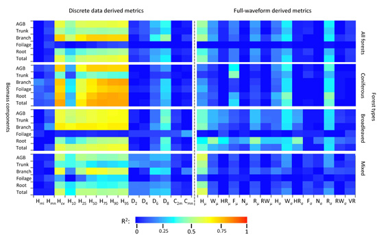

1. Introduction

As a primary reservoir of carbon dioxide (CO₂) in terrestrial ecosystems, forests play a key role in the global carbon cycle [1]. Globally, forest ecosystems contain approximately 80% of the world’s aboveground and 40% of belowground carbon stocks [2]. The subtropical forests biome accounts for approximately a quarter of the area of China and are particularly important for improving regional ecological environment and maintaining global carbon balance [3]. Despite their importance, there is still considerable uncertainty about carbon budgets within these subtropical forests, despite several national-scale studies using historical forest inventory data [4]. In addition, the partitioned biomass components (i.e., trunk, branch, foliage and root) also provide important information for forest management decisions such as the estimation of stem and branch biomass for biofuels calculations, as well as analyzing foliage biomass for studying forest growth and assessing crown biomass (i.e., branch and foliage biomass) for predicting fire hazard [5,6].

Remote sensing techniques can provide quantitative spatial explicit information and “wall-to-wall” observations for carbon stock mapping and monitoring [7]. However, since subtropical forests are typically structurally-complex and carbon-dense ecosystems, sensors (such as Landsat and shorter waveform RADAR, Radio Detection and Ranging) tend to saturate which inhibits reliable forest carbon stock estimates in these regions [8]. In addition, optical sensors can only provide limited information of the vertical structure of the forests [9]. Light Detection and Ranging (LiDAR) is an active remote sensing laser technology capable of providing detailed, spatially explicit, three-dimensional information on vegetation structure [10]. A large number of studies have demonstrated the potential of LiDAR to accurately estimate biophysical and structural properties over a wide range of forest types [11].

Over the past decades, many conventional airborne LiDAR systems produce small-footprint discrete data (system points) [12]. These systems record multi-returns (n ≤ 5) per transmitted pulse with each return representing the 3D position and intensity of the reflected light corresponding to the surfaces where the light has been reflected [13]. Discrete data can also be derived from the LiDAR waveforms (waveform points), which provide a denser point cloud in contrast to conventional systems [14]. However, research has indicated that the difference between the system versus waveform points for estimating canopy height is negligible, as the additional points (from waveform points) mainly describe the internal crown structure and the low vegetation stratum, and as a result the DTM and CHM-based heights are not significantly improved [15]. These discrete data-based approaches have been successfully used to describe a wide range of forest characteristics [16]. For instance, airborne LiDAR estimated tree heights were found to be of similar or better accuracy than corresponding field-based measurements [17]. Additional attributes, such as leaf area index [18], canopy volume [19] and biomass [20,21], are also well characterized with discrete LiDAR data at both the individual-tree and plot scale [22].

Due to limitations in the electronics of many conventional airborne LiDAR systems, only surfaces that are sufficiently spaced apart can be distinguished into separate returns [13]. Recently, small-footprint full-waveform LiDAR systems have become available commercially; these systems provide new opportunities for forestry studies [23]. These full-waveform systems digitize and record the entire backscattered signal of each emitted pulse, and allow the recording of detailed geometric and physical properties of intercepted objects [24]. The analysis of full-waveform data has improved height estimations [25], enhanced point extraction [26] and additional target information [15]. This extended return information has been successfully applied to forestry applications, such as single tree detection [27], tree species classification [28,29] and the estimation of forest structure characteristics [30,31].

In this paper, we examine the relationship between forest biomass (i.e., above-ground and total biomass) and its components (i.e., foliage, branch, trunk and root biomass) with small-footprint discrete (DR) and full-waveform (FW) airborne LiDAR derived metrics in three typical subtropical forest types (i.e., coniferous, broadleaved and mixed forests). In addition, we examine the estimation capability of DR and FW metrics based models for biomass estimation individually and in combination. Finally, the accuracy of the relationships is evaluated within each forest type by comparing biomass estimates with field measurements and characterizes the environments using additional topographic and vegetation conditions.

2. Materials and Methods

2.1. Study Site Description

Yushan Forest, a state-operated forest and national forest park, is located near the town of Changshu in Jiangsu province, southeast China (120°42′9.4″E, 31°40′4.1″N). It covers approximately 1103 ha, with an elevation range of approximately 20–261 m above sea level (Figure 1). This site is situated in the north-subtropical monsoon climatic region with an annual mean precipitation of 1062.5 mm; the highest monthly precipitation occurs in June (171 mm) and July (147 mm). The forest in Yushan belongs to the North-subtropical mixed secondary forest with three main forest types: coniferous-dominated, broad-leaved dominated and mixed forests [32]. The main conifers species include Masson pine (Pinus massoniana Lamb.) and Chinese fir (Cunninghamia lanceolata (Lamb.) Hook.) as the apex species, and a small percentage of Slash pine (Pinus elliottii Engelm.) and Japanese Blackbark Pine (Pinus thunbergii Parl.). The primary broad-leaved species are Sawtooth oak (Quercus acutissima Carruth.) and Chinese sweet gum (Liquidambar formosana Hance), mixed with some evergreen broad-leaved tree species belonging to the Fagaceae, Lauraceae and Theaceae.

2.2. Field Data

Using historical discrete return airborne LiDAR data (2007), a mean height and a cover layer at 30 m cell resolution were developed to be used as an initial stratification of the study area. The height and canopy layers were classified into five equal interval classes and in combination with the GIS-based forest inventory data (2012) to guide the selection of ground sample plot. A total of 65 square plots (30 × 30 m) were established within the study site, covering a range of species composition, age classes, and site indices. These plots were divided into three types based on species composition: (i) coniferous forest (n = 15, dominated by Masson pine and Chinese fir); (ii) broad-leaved forest (n = 18, dominated by Sawtooth oak and Chinese sweet gum); and (iii) mixed species forest (n = 32, a mixture of coniferous and broad-leaved species).

Plot data were collected during the 2012 (June to August) and 2013 (August) growing seasons under leaf-on conditions. Plot corners were located using Trimble GeoXH6000 Handheld GPS units, and the high precision real-time differential signals were received from the Jiangsu Continuously Operating Reference Stations (JSCORS), resulting in submeter accuracy [33]. At each plot, species of all measured trees and the status of the tree (live or dead), along with the crown class (e.g., dominant or co-dominant) were recorded. For all live trees with a DBH > 5 cm, diameter, height, height to crown base, and crown width in both cardinal directions were measured. Small trees (DBH < 5 cm) and dead wood were also tallied for total stem number, but not used in biomass calculations. DBH was measured on all trees using a diameter tape. Heights of all trees were measured using a Vertex IV hypsometer. Crown widths were determined by measuring two crown radii, one being the major axis (to the tip of the outmost branch on the longest side of the crown) and the other being 90° (perpendicular) to the first axis.

Several plot-level forest variables were calculated based on the individual tree data, including basal area (m²·ha⁻¹) and Lorey’s height (i.e., the basal area weighted height). Species-specific exponential allometric equations referenced from Feng et al. (1999) were used (Allometric equations developed from tree inventory data from local or nearby provinces were selected for this research) [34], with biomass (i.e., total and above-ground biomass) and biomass components (i.e., stem, root, branch and foliage) calculated for individual trees within each plot based on the field-measured DBH and height, and then summed to obtain total plot biomass. A summary of the derived ground biomass estimates is provided in

Table 1. Summary statistics of field measured biomass and biomass components in the study area (n = 65 plots).

Variables	Coniferous Forest (n = 15)			Broad-Leaved Forest (n = 18)			Mixed Forest (n = 32)
	Range	Mean	Std.Dev.	Range	Mean	Std.Dev.	Range	Mean	Std.Dev.
hL	4.47–12.97	9.56	1.87	7.70–18.52	12.28	2.83	7.79–14.18	10.55	1.55
G	10.21–57.70	25.92	10.24	21.12–78.59	39.15	17.05	16.95–60.57	29.49	10.75
WAGB	11.02–127.39	72.93	28.82	43.01–219.67	105.30	44.24	32.03–192.22	87.71	32.45
Wtrunk	8.35–84.55	53.05	19.48	29.16–173.05	79.11	34.73	18.65–174.09	68.84	28.13
Wbranch	1.62–25.12	10.54	7.02	9.72–44.46	20.52	9.66	4.09–25.33	12.31	5.73
Wfoliage	1.04–23.57	9.34	7.40	2.27–8.67	5.64	2.26	2.13–18.24	6.55	3.90
Wroot	6.25–39.42	22.03	8.18	20.21–45.62	29.98	6.71	10.31–61.90	26.49	9.63
Wtotal	12.06–150.95	82.27	34.72	45.27–223.85	110.94	44.65	34.16–197.57	94.26	34.09

Note: h_L: Lorey’s height (m); G: basal area (m²·ha⁻¹); W_AGB: above ground biomass (Mg·ha⁻¹); W_trunk: trunk biomass (Mg·ha⁻¹); W_branch: branch biomass (Mg·ha⁻¹); W_foliage: foliage biomass (Mg·ha⁻¹); W_root: root biomass (Mg·ha⁻¹); W_total: total biomass (Mg·ha⁻¹).

.

2.3. LiDAR Data

Small-footprint LiDAR data were acquired on 17 August 2013 using a Riegl LMS-Q680i scanner (which is a full-waveform digitizing laser scanner), onboard the LiDAR, CCD and Hyperspectral (LiCHy) Airborne Observation System [35]. The system was operated at 900 m above ground level, with a flight line side-lap of ≥60%. Data was acquired at a 400 kHz pulse rate with a scanning angle of ±30° from nadir (pulses transmitted at scan angles that exceeded 15° were excluded from the final dataset). The returned waveforms were recorded with a temporal sample spacing of 1 ns (approximately 15 cm) and beam footprint size around 0.25 m. The dataset had an average pulse spacing of 0.74 m and pulse density of 1.4 pulse·m⁻² in a single strip, with approximate three times higher pulse density in the overlapped regions.

Only one dataset was used for the entire analysis, the discrete data (with XYZ coordinates, intensities and additional parameters) were extracted from the full-waveform. The aim of this research is not to investigate the benefits of using the higher density point clouds provided by the full waveform laser scanning (see Reitberger et al. 2009 [36]), rather to explore how discrete and full-waveform data differ in their estimation of total biomass and specific biomass components. The discrete data were extracted using decomposition algorithms provided by the RIEGL RiAnalyze^® software (Horn, Austria). The algorithms are based on fitting one or multiple Gaussian pulses to the waveform data and extracting the temporal position (and range) of the pulses, the individual signal strength (amplitudes) and signal broadening (echo width) for each echo [37]. The full-waveform and discrete LiDAR data were both stored in LAS format (American Society for Photogrammetry and Remote Sensing, Bethesda, MD, USA) as final products by the data provider.

2.4. Data Pre-Processing

A 1-m digital terrain model (DTM) was created in two steps from the DR data: first, the data was filtered to remove the above-ground returns (using algorithm adapted from Kraus and Pfeifer, 1998) [38], and secondly the DTM was created by calculating the average elevation from the remaining (ground) LiDAR returns within a cell (cells that contain no points were filled by interpolation using neighboring cells). The DR point clouds were then normalized against the ground surface height and extracted for each plot using the coordinates of the lower left and upper right corners. All point cloud data processing was performed using the FUSION software package [39].

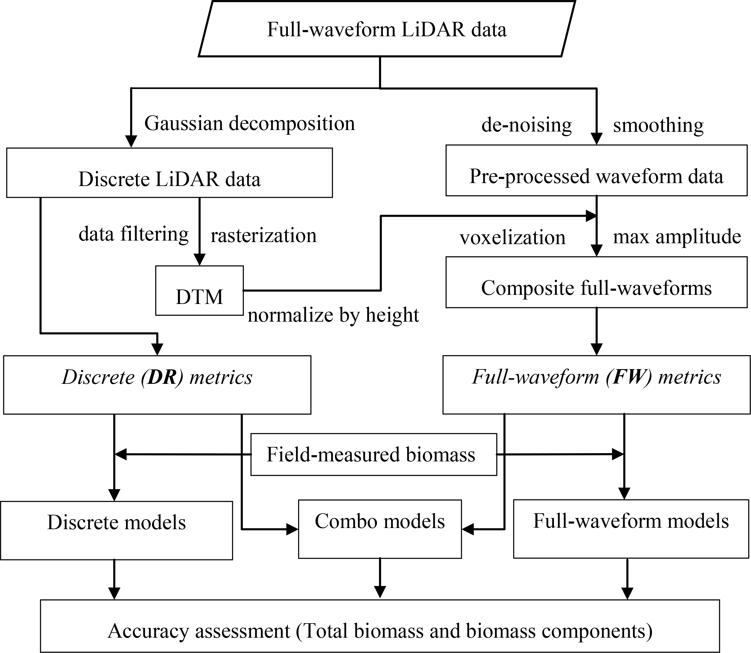
To avoid the effects of off-nadir pointing on the FW (e.g., the waveform is stretched as off-nadir angle increases) and to integrate non-vertical waveforms from different flight trajectories, a voxel-based approach developed by Hermosilla et al. (2014) was applied to the full-waveform data [40]. This approach synthesized multiple raw waveforms into composite waveforms through the vertical space partitioning of forest canopies by voxels, and uses the maximum amplitude value to construct new pseudo-vertical waveforms. The background noise of each waveform was first suppressed by a de-noising process and then smoothed by a Gaussian filter [40]. Each pre-processed waveform was then spatially located in the three-dimensional space and normalized by subtracting the derived DTM height from height of each bin in the corresponding positions. The vertical space was partitioned into voxels (0.25 × 0.25 × 0.15 m) according to the footprint size and temporal sample spacing. A maximum amplitude value was calculated and assigned to each intersected voxel. The composite waveforms were finally extracted as each vertical column of voxels [31] (See the technical route of this research in Figure 2).

2.5. LiDAR Metrics

2.5.1. Discrete Data Based Metrics

Discrete data based metrics are descriptive structure statistics calculated from the height normalized LIDAR point cloud measurements in three-dimensional space [41]. In this study, 15 metrics for each plot within the 30 × 30 m area of the 65 plots were calculated including: (i) selected height measures, i.e., percentile height (h₁₀, h₂₅, h₅₀, h₇₅, h₉₀ and h₉₅), maximum height (h_max) and mean height (h_mean); (ii) variability of height measures, i.e., coefficient of variation of heights (h_cv); (iii) selected canopy return density measures, i.e., canopy return density (d₂, d₄, d₆ and d₈) and (iv) canopy cover measures, i.e., canopy cover above 2 m (CC_2m) and canopy cover above mean height (CC_mean).

All of the discrete data-based metrics were generated from first returns, which have been found to be more stable for estimating forest biophysical attributes than all returns [42]. Metrics of heights and canopy return densities were computed with a height threshold of 2-m above ground-level to ensure that the non-canopy and below-canopy returns were excluded from metric calculation [43,44].

2.5.2. Full-Waveform Based Metrics

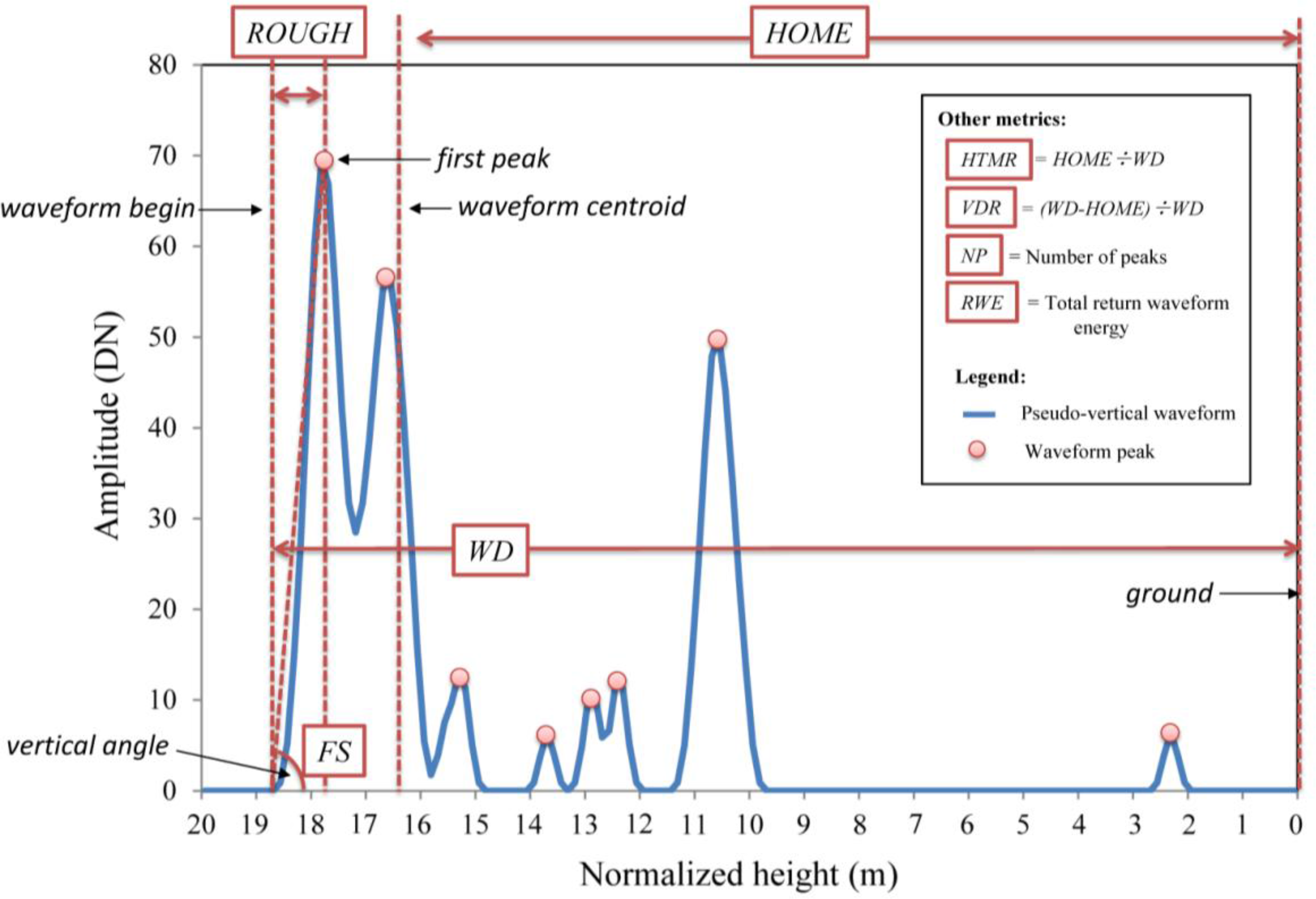
Full-waveform data based metrics describe the radiometric and geometric attributes of the return waveforms based on the spatio-temporal analysis [40]. In this research, 15 waveform metrics adapted from previous studies of large-footprint full-waveform data (i.e., SLICER, LVIS and GLAS) were incorporated into the pseudo-vertical waveform analysis due to their success in previous studies [28–31,45]. These metrics include height of median energy (HOME), waveform distance (WD), height/median ratio (HTMR), number of peaks (NP), roughness of outermost canopy (ROUGH), front slope angle (FS), return waveform energy (RWE) and vertical distribution ratio (VDR) (Figure 3).

HOME is calculated as the distance from waveform centroid to the ground (i.e., corresponding DTM height), and has been found to be sensitive to canopy openness and the vertical arrangement of canopy elements [46]. WD, often related to the LiDAR canopy height, is computed as the distance from waveform begin to the ground [47]. HTMR, which is the HOME divided by the WD, was used to depict the change of HOME relative to the canopy height [46]. ROUGH, which is the distance from the waveform beginning to the first peak, was applied to describe the roughness of the upper-most canopy and the spatial arrangement of plant surfaces [25,48]. FS, which is the vertical angle from waveform beginning to the peak of canopy return energy, provides the variability of the upper canopy [49]. NP is the number of detected peaks within each composite waveform. RWE represents the total received energy. VDR is calculated as the differences between the WD and the HOME, divided by WD [30]. The plot level waveform metrics (except VDR) were summarized as the mean and standard deviation of all the waveform metrics (of individual composite waveform) within each plot. A summary of the metrics with corresponding descriptions is shown in

Table 2. Summary of LiDAR metrics computed from discrete and full-waveform LiDAR data.

Metrics	Description
Discrete LiDAR Data (n = 15)
Percentile height (h10, h25, h50, h75, h90, h95)	The percentiles of the canopy height distributions (10th, 25th, 50th, 75th, 90th, 95th) of first returns
Canopy return density (d2, d4, d6, d8)	The canopy return density over a range of relative heights, i.e., percentage (0%–100%) of first returns above the quantiles (20, 40, 60, 80) to total number of first returns
Minimum height (hmin)	Minimum height above ground of all first returns
Maximum height (hmax)	Maximum height above ground of all first returns
Coefficient of variation of heights (hcv)	Coefficient of variation of heights of all first returns
Canopy cover above 2 m (CC2m)	Percentage of first returns above 2 m.
Canopy cover above mean (CCmean)	Percentage of first returns above the first return mean heights.
Full-Waveform LiDAR Data (n = 15)
HOME_mean (HOMEμ)	Average of height of median energy
HOME_stdev (HOMEσ)	Standard deviation of height of median energy
WD_mean (WDμ)	Average of waveform distance
WD_ stdev (WDσ)	Standard deviation of waveform distance
HTMR_mean (HTMRμ)	Average of height: median ratio
HTMR_stdev (HTMRσ)	Standard deviation of height: median ratio
NP_mean (NPμ)	Average of number of peaks
NP_stdev (NPσ)	Standard deviation of number of peaks
ROUGH_mean (ROUGHμ)	Average of roughness of outermost canopy
ROUGH_ stdev (ROUGHσ)	Standard deviation of roughness of outermost canopy
FS_mean (FSμ)	Average of front slope angle
FS_stdev (FSσ)	Standard deviation of front slope angle
RWE_mean (RWEμ)	Average of return waveform energy
RWE_ stdev (RWEσ)	Standard deviation of return waveform energy
VDR (VDR)	Vertical distribution ratio

.

2.6. Statistical Analyses

The strength of relationships between biomass (and each biomass components) and the 30 LiDAR metrics were tested by the square of the Pearson correlation coefficient (R²). Multiple linear regression models, which include the two sets of LIDAR metrics (i.e., discrete and full-waveform based metrics) as predictor variables, were developed independently and in combination for estimating the biomass and biomass components among different forest types (i.e., all forests, coniferous forests, broadleaved forests and mixed forests). To ensure the independent variables were not highly correlated, collinearity was first evaluated using Principal Component Analysis (PCA) based on the correlation matrix. Models with condition number (κ) lower than 30 were accepted to ensure that there was no serious collinearity in the selected models [50,51]. Standard backward stepwise regression was performed to select variables for the final models with predictor variables left in the models at the 5% significance level. The best fitting models were then selected based on the lowest Akaike information criterion value [52]. Once the best models were chosen, leave-one-out cross validation was used to validate them.

Three sets of predictive models, i.e., discrete data metrics based model (DR-model), full-waveform metrics based model (FW-model) and Combo model (includes the combination of both discrete and full-waveform metrics) were fitted. These prediction models were assessed using adjusted coefficient of determination (Adj-R²), Cross-validation coefficient of determination (CV-R²), Root-Mean-Square Error (RMSE), and relative RMSE (rRMSE), defined as the percentage of the ratio of RMSE and the observed mean values (

Table 3. The accuracy assessment results of three sets of predictive models among various forest types.

	Discrete Data Model				Full-Waveform Model				Combo Model
	Aj-R2	C-R2	RMSE	rRMSE	Aj-R2	C-R2	RMSE	rRMSE	Aj-R2	C-R2	RMSE	rRMSE
All forests
WAGB	0.7	0.65	20.12	22.7	0.52	0.45	25.36	28.61	0.71	0.65	19.91	22.46
Wtrunk	0.59	0.55	18.94	28.27	0.45	0.41	21.88	32.66	0.6	0.56	18.71	27.93
Wbranch	0.77	0.71	3.97	27.46	0.65	0.62	4.87	33.68	0.79	0.74	3.76	26.01
Wfoliage	0.29	0.23	4.02	56	0.07	0.04	4.59	63.94	0.32	0.28	3.91	54.47
Wroot	0.59	0.55	5.68	21.71	0.42	0.38	6.79	25.95	0.56	0.51	5.88	22.47
Wtotal	0.7	0.64	21.11	22.03	0.5	0.43	27.12	28.3	0.7	0.64	20.88	21.79
Coniferous forests
WAGB	0.84	0.79	11.55	15.84	0.81	0.76	12.45	17.07	0.92	0.87	8.08	11.08
Wtrunk	0.5	0.46	13.78	25.98	0.65	0.61	11.49	21.66	0.84	0.81	7.78	14.67
Wbranch	0.88	0.81	2.45	23.25	0.77	0.73	3.36	31.89	0.93	0.88	1.84	17.46
Wfoliage	0.79	0.73	3.38	36.18	0.73	0.69	3.84	41.1	0.82	0.78	3.12	33.39
Wroot	0.86	0.82	3.04	13.8	0.76	0.71	3.97	18.02	0.88	0.85	2.82	12.8
Wtotal	0.88	0.83	11.83	14.38	0.79	0.73	15.9	19.33	0.93	0.89	9.29	11.29
Broadleaved forests
WAGB	0.87	0.84	16.23	15.41	0.58	0.52	28.83	27.38	0.86	0.81	16.31	15.49
Wtrunk	0.87	0.83	12.55	15.86	0.57	0.53	22.74	28.75	0.89	0.85	11.34	14.33
Wbranch	0.88	0.82	3.34	16.27	0.61	0.56	6.06	29.53	0.89	0.84	3.23	15.74
Wfoliage	0.18	0.13	2.05	36.36	0.27	0.22	1.93	34.23	0.33	0.29	1.85	32.81
Wroot	0.63	0.57	4.08	13.61	0.43	0.38	5.06	16.88	0.65	0.61	4.0	13.34
Wtotal	0.84	0.81	17.84	16.08	0.57	0.51	29.3	26.41	0.84	0.79	18.14	16.35
Mixed forests
WAGB	0.75	0.72	16.08	18.33	0.59	0.53	20.85	23.77	0.82	0.78	13.94	15.89
Wtrunk	0.67	0.61	16.1	23.39	0.53	0.49	19.27	27.99	0.77	0.72	13.42	19.49
Wbranch	0.72	0.65	3.02	24.53	0.58	0.54	3.72	30.21	0.71	0.66	3.08	25.01
Wfoliage	0.44	0.41	2.92	44.56	0.41	0.37	3.01	45.93	0.48	0.43	2.77	42.27
Wroot	0.7	0.64	5.3	20.01	0.44	0.40	7.19	27.14	0.73	0.68	4.99	18.84
Wtotal	0.75	0.71	16.89	17.92	0.63	0.58	20.85	22.12	0.81	0.76	14.94	15.85

Note: Aj-R²: adjusted R-square; C-R²: The cross-validation coefficient of determination; RMSE: Root mean square error; rRMSE (%): relative RMSE, i.e., percentage of the ratio of RMSE and the observed mean value. See Table 1 for codes of biomass and its components.

).

3. Results

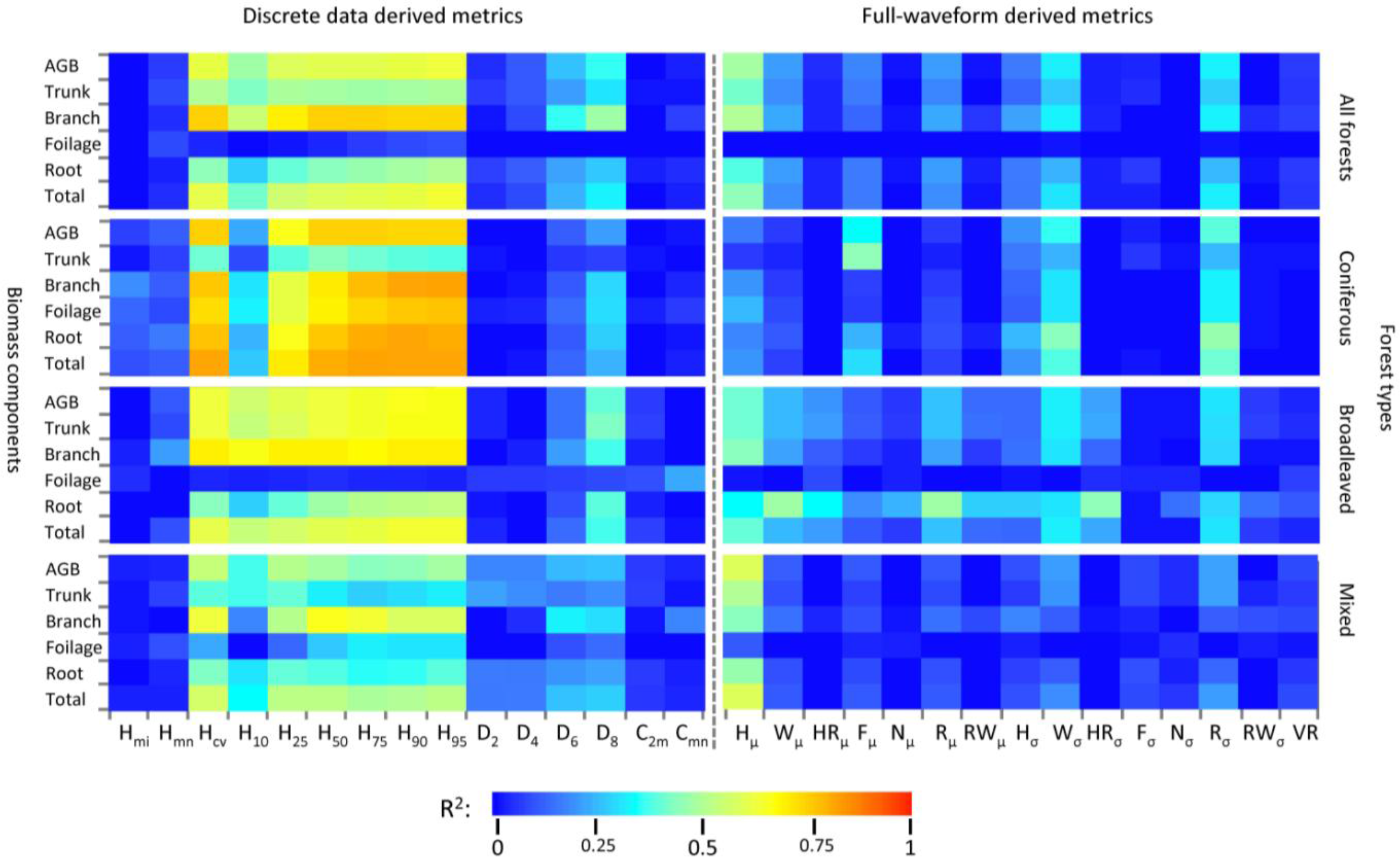
Most of the biomass and its components (hereafter written as “biomass components”) have a stronger correlation with the discrete data based metrics than the waveform model based metrics (Figure 4). Within the set of discrete data based metrics, except for the “all forests” and “broadleaved forests” foliage biomass components, most of the height-related metrics (especially the percentile heights and the coefficient of variation of heights) and biomass components are strongly correlated. In comparison, measures of canopy return density and canopy cover have a relatively poorer relationship with the biomass components. The strength of the relationships between biomass components and the waveform metrics were also generally weaker. The waveform metrics related to canopy height (e.g., WD), vertical arrangement (e.g., HOME) and roughness of upper-most canopy (e.g., ROUGH) had a more significant relationship with biomass components than others.

Details on the three sets of predictive models (i.e., general and forest-type specific models developed from discrete data based metrics, waveform based metrics and their combinations) are shown in Tables A1–A3 and Table 3 summarizes their accuracies. Overall, most of the biomass components are generally well predicted (Adj-R² = 0.42–0.93, rRMSE = 11.08%–33.68%) except for foliage biomass (Adj-R² = 0.07–0.82, rRMSE = 32.81%–62.94%). The combo models performed the best; explaining 60%–79% (for the general model) and 65%–93% (for each forest type-specific model) of the variability of most biomass components (exclude foliage biomass). Compared with full-waveform models (Adj-R² = 0.42–0.79, rRMSE = 16.88%–33.68%), the discrete data models (Adj-R² = 0.50–0.88, rRMSE = 13.61%–28.27%) have a relatively higher performance, except for the trunk biomass (in coniferous forests) and foliage biomass (in broadleaved forests) (see Table 3). The fit for the general model (developed from all plots) is relatively low (Adj-R² = 0.07–0.79). In comparison, the relationship were generally improved for forest type-specific models (Adj-R² = 0.18–0.93). Overall, most of the fitted models had higher correlations in coniferous forests (Adj-R² = 0.50–0.93) and broadleaved forests (Adj-R² = 0.43–0.89) than in mixed forest types (Adj-R² = 0.41–0.82). The relative RMSE was generally in accordance with adjusted R², with lower values in coniferous forests (rRMSE = 11.08%–41.1%) and broadleaved forests (rRMSE = 13.34%–36.36%) than in mixed forest types (rRMSE = 15.85%–45.93%).

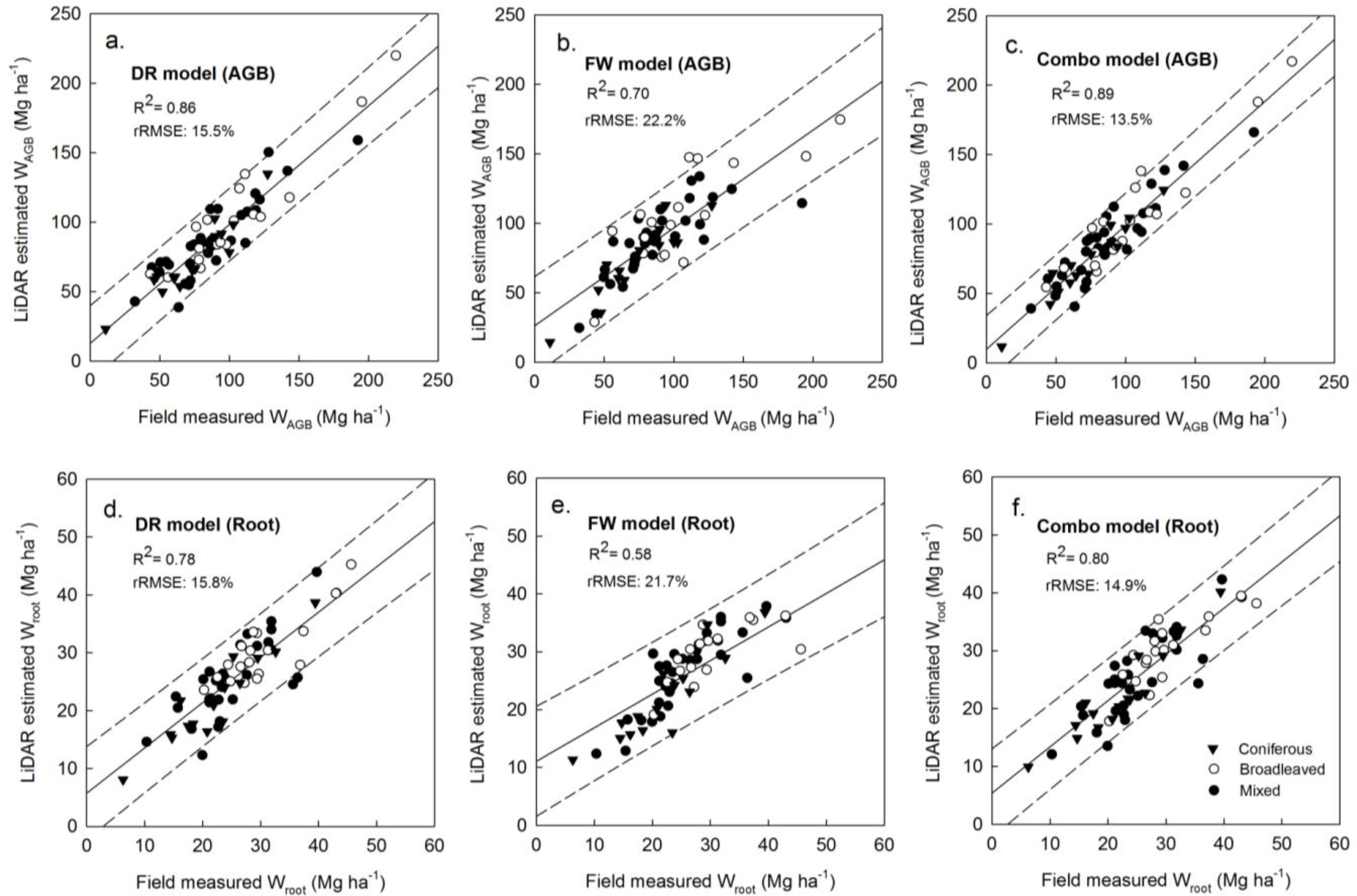
Scatter plots of the plot-level field-measured and LiDAR-estimated above-ground and root biomass are shown in Figure 5 with linear fits and prediction confidence intervals (95%). The linear models demonstrate the increased correlations in the Combo models (R² = 0.89 for above-ground biomass; R² = 0.80 for root biomass) in comparison to the DR model (R² = 0.88; R² = 0.78) and FW model (R² = 0.70; R² = 0.58). The widths of the confidence intervals in the DR model (AGB) and Combo model (AGB) are relatively narrow, indicating better quality of model fitting. Some outliers, which may be the result of prediction bias, should be noted in the FW model (AGB) and DR model (Root).

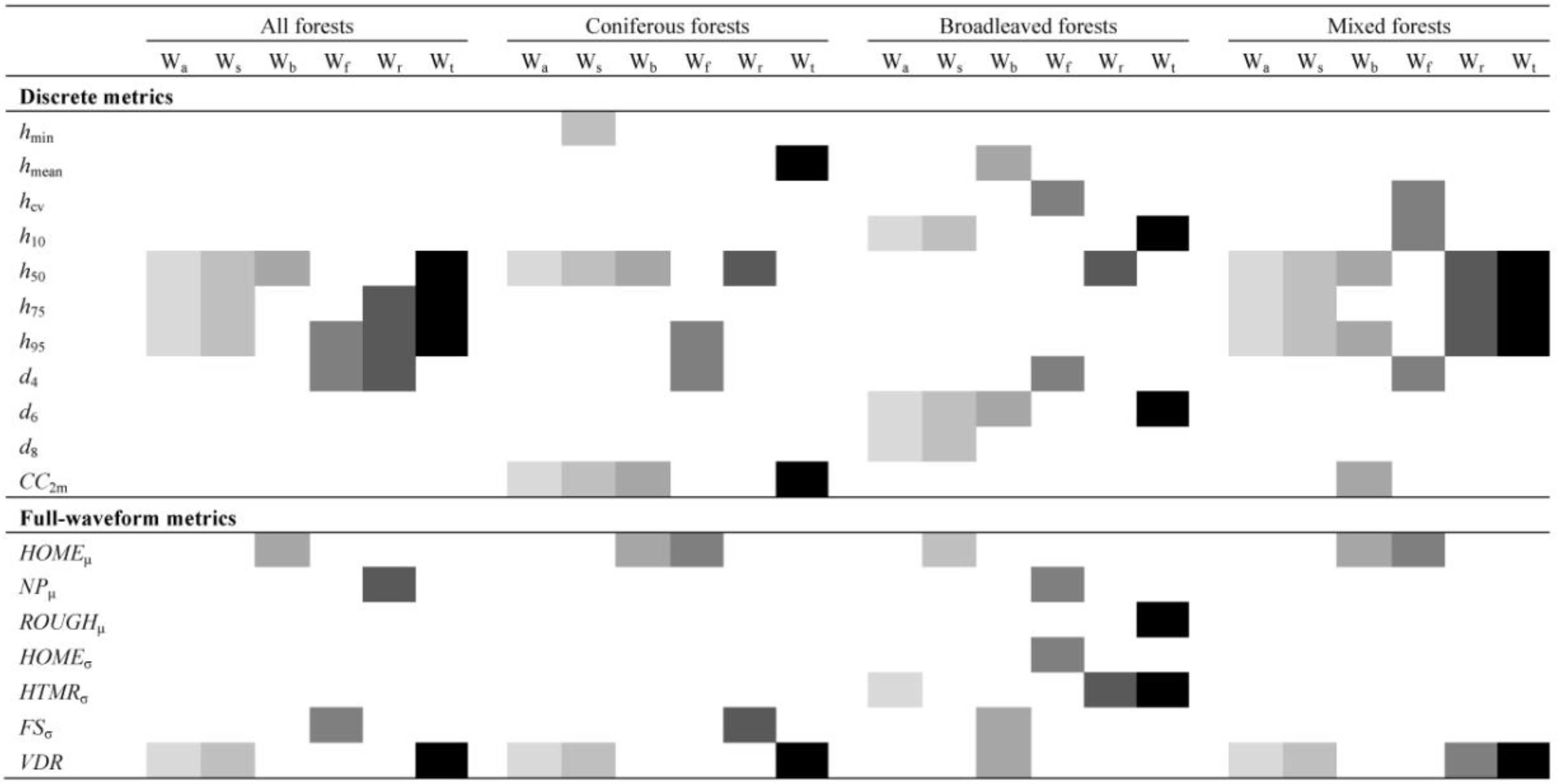
The selected metrics of the two sets of biomass estimation models (i.e., the discrete data models and full-waveform models) are shown in Figure 6. For the discrete data models, height-related metrics (h_mean, h₅₀, h₇₅ and h₉₅) calculated from the point cloud are the most frequently selected by the regression models, followed by canopy return density and canopy cover metrics. The h_mean statistic is sensitive to all of the biomass components in coniferous forests (selected by all of the 6 conifer models). In comparison, the statistics of h₅₀ and h₉₅ are more sensitive to the biomass components of “all forests” and mixed forests (selected by 8–9 of 12 models of the “all forests” and mixes), whereas d₆ and d₈ are more sensitive to the biomass components of broadleaved forests (selected by 5 of 6 models of the broadleaves). The h₇₅ statistic appears sensitive to above-ground (W_AGB), trunk (W_trunk) and total biomass (W_total), often selected by the predictive models (in 3 of the 4 forest types). For the full-waveform models, the statistic of HOME_μ calculated from composite waveforms is the most frequently selected variable. The HTMR_μ and NP_μ statistics appear sensitive to foliage biomass since they are selected to predict this component in 3–4 of the 4 forest types. FS_σ are significantly sensitive to the branch biomass since they are selected in 4 of all the forest types.

Figure 7 represents the selected metrics of the combo models, i.e., using both discrete and full-waveform metrics. Each predictive model includes at least one variable from the DR and FW metric pools, whereas more discrete metrics (11 out of the total 15) are used in the combo models than full-waveform metrics (7 out of 15). Height-related metrics of h₅₀ and h₉₅ remain sensitive to the biomass components of “all forests” and mixed forests (selected by 8–9 of 12 models of the “all forests” and mixes), which agrees with the previous analysis of the discrete data only models. VDR is the most frequently used full-waveform metrics in the combo models (it is selected at least once for each forest type-specific models).

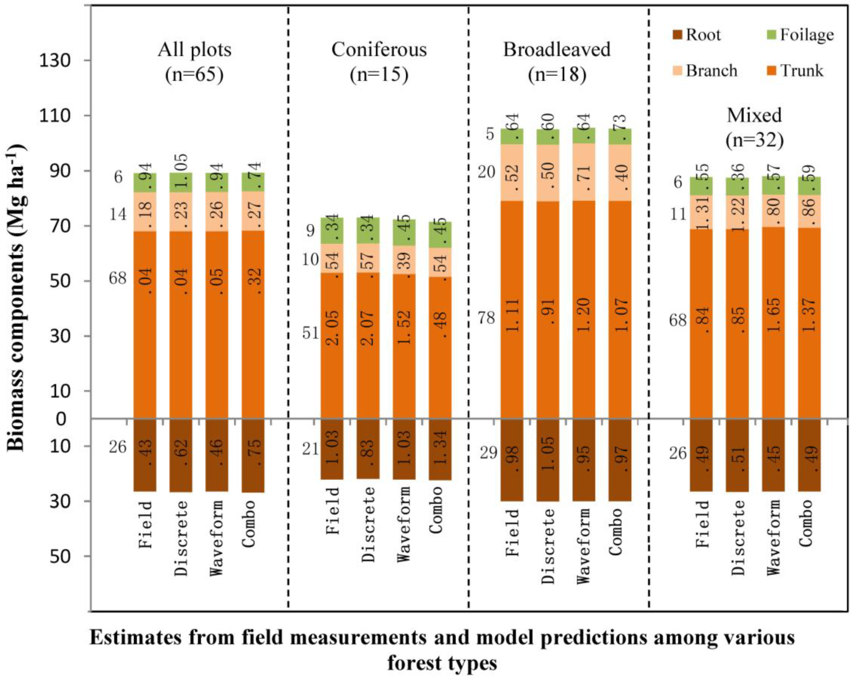
Within specific forest types, the biomass components were calculated using the individual models (i.e., forest type-specific models) and then averaged (Figure 8). Compared with the field measurements (the first left column in each forest type), most of the biomass components were similar to the field-measured values except for an overestimation of branch biomass by all the models within all plots; an underestimation of trunk biomass by full-waveform and combo models within coniferous forests; and an overestimation of trunk biomass by full-waveform and combo models within the mixed forests.

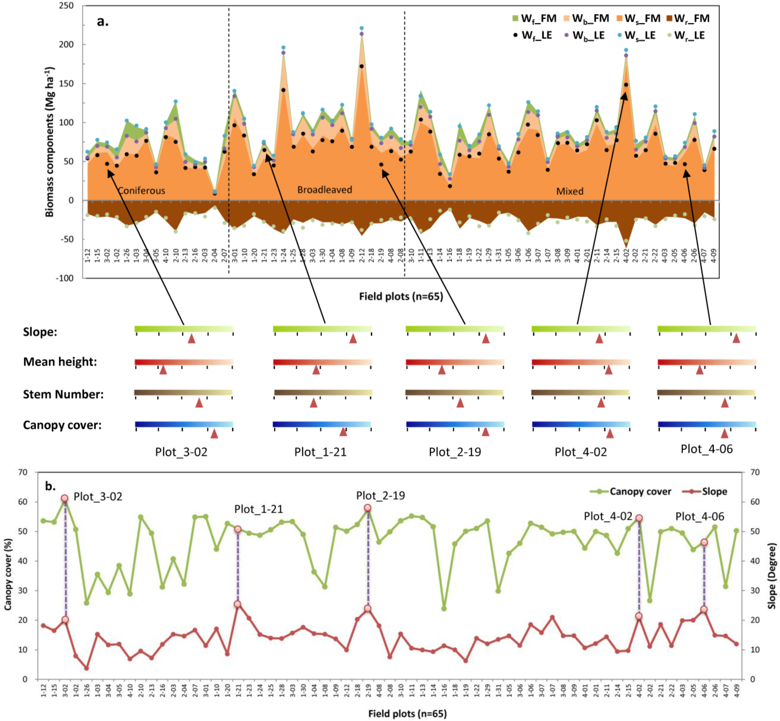
Across all 65 field plots, the relationship between field-measured and LiDAR-estimated biomass components is shown in Figure 9. Overall, most of the estimated biomass components of foliage, branch and root are well predicted by the combo models. Five plots with the largest bias in trunk biomass are highlighted and analyzed against four topographic and vegetation factors which may influence the accuracy of biomass estimation [53–55]. Both slope (calculated by DTM) and canopy cover (Percentage of first returns above the first return 2-m heights) were derived from discrete LiDAR data, while the mean height and stem number of trees were calculated based on the field-measured data. All five plot outliers have high levels of canopy cover, and most are located on steep slopes (Figure 9b).

4. Discussion

In similar forests, Fu et al. (2011) estimated above-ground biomass components using low hit density (point distance = 1.08 m) small foot-print discrete LiDAR data in 78 smaller circle plots (radius = 7.5 m or 15 m) in mountainous subtropical forests, southwest China [56]. Compared with our results, less variability was explained for above-ground biomass within those broad-leaved (43%) and coniferous (68%) forests, and there was no significant correlation found in the mixed forests. Both the larger plot size (see Zhao et al. 2009 for details on the effects of plot size) [57] and the higher hit density may explain the more significant correlations found in this study. Studies predicting root biomass from small footprint LiDAR especially in subtropical forest are rare. Næsset, (2004) reported a R² = 0.86 for below-ground biomass in boreal forests [58]. Pang and Li (2012) fitted regression models for biomass components in temperate forests in Northeast China and explained 85% of the variability in root biomass in conifers, which is slightly higher than reported in this study [59]. The reason for the slightly lower accuracy in our study may be because of the complexity of multilayered subtropical forest, which has a far greater variability in stem height and density compared to boreal and temperate forests.

Neuenschwander et al. (2012) extracted waveform metrics (e.g., amplitude, pulse width, integrated canopy energy) from FW data and found that the FW-metrics can help improving the characterization and classification of the vegetation [30]. In this study, Most of the combo models (include both DR and FW metrics) show a higher variation explanation capability for predicting the biomass components than the DR-metrics (only) models, especially for of trunk biomass (in coniferous forests; with a adjusted-R² increase of 0.34) and foliage biomass (in broadleaved forests; with a adjusted-R² increase of 0.15), which is in agreement with their findings. Sumnall et al. (2012) investigated the estimation of forest structural variables from both discrete (system points) and full waveform LiDAR data [60]. Height and intensity-related metrics were derived from DR data (system points), metrics of heights (derived from waveform points), amplitude and pulse widths of the waveforms were all derived from FW data. Results indicated that most of the FW-models (using both waveform points and full-waveform based metrics as independent variables) had a higher accuracy than DR models (using system points based metrics as independent variables) for estimating biophysical properties of a semi-natural forest in southern England, which agrees with our research which shows that most of the combo models had a higher performance than DR-models, and the full-waveform metrics contribute to the improvements by characterizing the detailed vertical structure of the forest stands.

For the discrete and full-waveform metrics analyzed in this study, these metrics related to vegetation heights, i.e., mean height, upper height percentiles (i.e., h₅₀, h₇₅, h₉₅), HOME (i.e., waveform centroid to the ground) and VDR (calculated from HOME and waveform distance), were the strongest predictors of biomass and its components. Larson (1963) found that the bole form and stem increment are strongly connected to the crown geometry and crown position [61]. The LIDAR sensors measure 3-D structure characteristics of the forest canopy, which provides a good foundation for strong relationships between the LIDAR-derived metrics and forest biomass. Since most LiDAR returns are from dominant trees, the LiDAR mean height likely represents the height of overstory trees. The inclusion of waveform-derived HOME (which depicts the vertical arrangement of canopy elements) and VDR (describes the change of HOME relative to the canopy height) [25], helps to account for intermediate tree crowns in the midstory and suppressed trees in the understory, therefore potentially improving the characterizing of vertical structure. The predictive capabilities of these metrics are strong (in both the single and combo models) for estimating most of the biomass components, and they therefore provide a precise quantitative description of stand structure characteristics. This finding is consistent with the small-footprint discrete data [20], small-footprint full-waveform data [31,40] and large-footprint SLICER data [41,46] studies, in which mean height, height percentiles and HOME (and HOME-related waveform metrics) were found to explain most of variability in forest structure characteristics.

Compared to the individual DR and FW models, the combo models performed the best, explaining a large amount of variability for most biomass components, and indicating significant synergies in small-footprint DR and FW LiDAR data across the three types of subtropical forests. Fu et al. (2011) explored several regression models relating both percentile heights and canopy return density variables derived from airborne DR LiDAR for the estimation of above-ground biomass components in a similar forest type [56]. Compared with our study, their results showed relatively low relationships for above ground biomass (R² = 0.37–0.68), and no significant correlation between foliage biomass and the DR metrics in the subtropical mixed forests. In this study, FW models have a higher variation explanation capability for predicting foliage biomass than DR models. The waveform statistic of HTMR_μ and NP_μ also seems to be sensitive to foliage biomass, and FS_σ are significantly sensitive to the branch biomass. The results demonstrate promising results for improving the estimation of crown (i.e., branch and foliage) components, which would be useful for modeling forest growth and fire behavior.

In this study, the forest type-specific models represent a better performance than the general model (developed from all plots). This is consistent with the previous studies which demonstrate that forests with highly variable species composition should be stratified to ensure accurate biomass predictions [56,59]. Næsset (2004) reported that forest type did not have any significant impact on the estimated biomass models in boreal forest (in southeast Norway, dominated by Norway spruce and Scots pine) [58]. However, in our study, the complex forest conditions in subtropical forests contained greater species diversity, making the effects of tree-species composition (classified as forest types) significant. Overall, the models were more accurate for coniferous and broadleaved forests than in mixed forests across all models. The dominating coniferous and broadleaved species in our research site have a relatively even-aged tree structure and higher homogeneous composition, i.e., less variation in tree height and density at the plot level. In contrast, the mixed forest has more variability and less accurate LiDAR-derived heights within plots. Meanwhile, individual tree biomass in coniferous and broadleaved plots was calculated by relatively accurate species-specific allometric equations, while the mixed forest biomass was estimated from a less accurate, generalized allometric equation. Thus, the homogeneous forest conditions coupled with the accurate field-measured biomass is expected to strengthen the linear fit and reduce bias.

Bater and Coops (2009) explored the relationship between the satellite-derived NDVI and LiDAR ground return density in a coastal western hemlock dominated forest, and found that ground return density decreased as NDVI (an estimate of vegetation cover) increased [55]. Clark et al. (2004) also demonstrated that, in an evergreen tropical rain forest, RMS error of DEM on steep slopes was 0.67 m greater than on flat slopes [53]. Meanwhile, the LiDAR ground retrieval was complicated by dense, multi-layered evergreen canopy in old-growth forests, causing an overestimation of 1.95 m. In this study, five plots with the largest bias of trunk biomass were analyzed by the factors of topographic and vegetation conditions. It was found that all of the five plot outliers had high levels of canopy cover, and most were located on steeper slopes. Thus, the lower predictive accuracy may due to less canopy penetration by LiDAR and consequently less accurate definition of the digital terrain model and canopy height model. Bater and Coops (2009) suggested that in those areas with high slope and low point density, the prediction uncertainty maps may provide insights into optimal DEM selection and improve the vegetation height estimation [55].

5. Conclusions

This study implemented two different approaches i.e., discrete data (DR) and full-waveform (FW) based approaches to extract plot-level LiDAR metrics, and evaluated the capacity of these metrics in predicting biomass and its components in three types of subtropical forests. The results indicated that the three sets of predictive models performed well across the different subtropical forest types (Adj-R² = 0.42–0.93, excluding foliage biomass). Forest type-specific models (Adj-R² = 0.18–0.93) were generally more accurate than the general model (Adj-R² = 0.07–0.79) with the most accurate results obtained for coniferous stands (Adj-R² = 0.50–0.93) in homogeneous forest conditions. In addition, the analysis of bias in the estimation of trunk biomass demonstrated that the lower accuracy may be due to less canopy penetration by the LiDAR returns, resulting in a less accurate digital terrain model and canopy height model.

According to the results, for the discrete and full-waveform metrics analyzed in this study, metrics related to vegetation heights, i.e., mean height, upper height percentiles, HOME and VDR, were the strongest predictors of biomass and its components. The FW-metrics were sensitive to the trunk biomass (in coniferous forests) and foliage biomass (in broadleaved forests). The results also demonstrated that most of the combo models (coupling of both FW and DR metrics) had improved performance than DR (only) models, and the FW metrics contributed to the improvements by characterizing the detailed vertical structure of the forest stands.

This study suggests that although the discrete and full-waveform LiDAR data extract forest canopy information in different ways, i.e., discrete data characterize the 3-D canopy structure, while full-waveform data recorded the detailed geometric and radiometric information of the canopy return, both discrete and full-waveform metrics can provide valuable information for accurately estimating specific biomass components in certain forest type of the subtropical forests. However, one should note that the choice of LiDAR metrics does impact the performance of models used for the biomass estimation, and different biomass pools are correlated with different LIDAR metrics. As a result, the combination of DR and FW metrics and the exploration of new sets of full-waveform metrics contributed to the development of more robust predictive models.

LiDAR biomass estimation has been conducted in temperate and boreal forests and the transition region of these forests [62–64]. Published studies from tropical (and subtropical) forests are few. As a result, this study contributes to the accurate and quantitative estimation of biomass using state-of-the-art airborne LiDAR technology in the subtropical forests. In addition, to our best knowledge, this is the first time different forest biomass components (of the subtropical forests) have been tested and estimated by the pseudo-vertical waveform analysis approach.

Future works should focus on exploring more full-waveform metrics derived from the small-footprint full-waveform LiDAR data using the pseudo-vertical waveform analysis approach. For a improved (and direct) interpretability of the full-waveform derived variables, the full-waveform information could be aggregated at the individual tree level, and validated with field measurements at this fine spatial scale. This proposed work could provide a bridge between crown delineation algorithms and pseudo-vertical waveform analysis approaches, and would be useful for individual-tree based biophysical properties estimation and tree-species classification.

References

- Pan, Y.; Birdsey, R.A.; Fang, J.; Houghton, R.; Kauppi, P.E.; Kurz, W.A.; Phillips, O.L.; Shvidenko, A.; Lewis, S.L.; Canadell, J.G.; et al. A large and persistent carbon sink in the world’s forests. Science 2011, 333, 988–993. [Google Scholar]
- Dixon, R.K.; Brown, S.; Houghton, R.A.; Solomon, A.M.; Trexler, M.C.; Wisniewski, J. Carbon pools and flux of global forest ecosystems. Science 1994, 263, 185–190. [Google Scholar]
- Wang, X.H.; Kent, M.; Fang, X.F. Evergreen broad-leaved forest in Eastern China: Its ecology and conservation and the importance of resprouting in forest restoration. For. Ecol. Manag 2007, 245, 76–87. [Google Scholar]
- Fang, J.; Chen, A. Dynamic forest biomass carbon pools in China and their significance. Acta Bot. Sin 2001, 43, 967–973. [Google Scholar]
- Lambert, M.C.; Ung, C.H.; Raulier, F. Canadian national tree aboveground biomass equations. Can. J. For. Res 2005, 35, 1996–2018. [Google Scholar]
- Saatchi, S.; Halligan, K.; Despain, D.G.; Crabtree, R.L. Estimation of forest fuel load from radar remote sensing. IEEE Trans. Geosci. Remote Sens 2007, 45, 1726–1740. [Google Scholar]
- Gibbs, H.K.; Brown, S.; Niles, J.O.; Foley, J.A. Monitoring and estimating tropical forest carbon stocks: Making REDD a reality. Environ. Res. Lett 2007, 2, 1–13. [Google Scholar]
- Lu, D.; Chen, Q.; Wang, G.; Moran, E.; Batistella, M.; Zhang, M.; Vaglio Laurin, G.; Saah, D. Aboveground forest biomass estimation with landsat and lidar data and uncertainty analysis of the estimates. Int. J. For. Res 2012, 2012, 1–16. [Google Scholar]
- Wulder, M.A. Optical remote sensing techniques for the assessment of forest inventory and biophysical parameters. Process Phys. Geogr 1998, 22, 449–476. [Google Scholar]
- Lefsky, M.A.; Cohen, W.B.; Parker, G.G.; Harding, D.J. Lidar remote sensing for ecosystem studies. Bioscience 2002, 52, 19–30. [Google Scholar]
- Dubayah, R.; Drake, J. Lidar remote sensing for forestry. J. For 2000, 98, 44–46. [Google Scholar]
- Lindberg, E.; Olofsson, K.; Holmgren, J.; Olsson, H. Estimation of 3D vegetation structure from waveform and discrete return airborne laser scanning data. Remote Sens. Environ 2012, 118, 151–161. [Google Scholar]
- Parrish, C.E.; Jeong, I.; Nowak, R.D.; Smith, R.B. Empirical comparison of full-waveform lidar algorithms: Range extraction and discrimination performance. Photogramm. Eng. Remote Sens 2011, 77, 825–838. [Google Scholar]
- Reitberger, J.; Krzystek, P.; Stilla, U. Analysis of full waveform LiDAR data for the classification of deciduous and coniferous trees. Int. J. Remote Sens 2008, 29, 1407–1431. [Google Scholar]
- Chauve, A.; Vega, C.; Durrieu, S.; Bretar, F.; Allouis, T.; Pierrot Deseilligny, M.; Puech, W. Advanced full-waveform lidar data echo detection: Assessing quality of derived terrain and tree height models in an alpine coniferous forest. Int. J. Remote Sens 2009, 30, 5211–5228. [Google Scholar]
- Lim, K.; Treitz, P.; Wulder, M.; St-Onge, B.; Flood, M. LiDAR remote sensing of forest structure. Prog. Phys. Geogr 2003, 27, 88–106. [Google Scholar]
- Næsset, E.; Økland, T. Estimating tree height and tree crown properties using airborne scanning laser in a boreal nature reserve. Remote Sens. Environ 2002, 79, 105–115. [Google Scholar]
- Morsdorf, F.; Kötz, B.; Meier, E.; Itten, K.; Allgöwer, B. Estimation of LAI and fractional cover from small footprint airborne laser scanning data based on gap fraction. Remote Sens. Environ 2006, 104, 50–61. [Google Scholar]
- Coops, N.C.; Hilker, T.; Wulder, M.A.; St-Onge, B.; Newnham, G.J.; Siggins, A.; Trofymow, J.A.T.A. Estimating canopy structure of Douglas-fir forest stands from discrete-return LiDAR. Trees-Struct. Funct 2007, 21, 295–310. [Google Scholar]
- Popescu, S.C. Estimating biomass of individual pine trees using airborne lidar. Biomass Bioenergy 2007, 31, 646–655. [Google Scholar]
- Cao, L.; Coops, N.; Innes, J.; Dai, J.; She, G. Mapping above- and below-ground biomass components in subtropical forests using small-footprint LiDAR. Forests 2014, 5, 1356–1373. [Google Scholar]
- Wulder, M.A.; Bater, C.; Coops, N.C.; Hilker, T.; White, J.C. The role of LiDAR in sustainable forest management. For. Chron 2008, 84, 807–826. [Google Scholar]
- Mallet, C.; Bretar, F. Full-waveform topographic lidar: State-of-the-art. ISPRS J. Photogramm. Remote Sens 2009, 64, 1–16. [Google Scholar]
- Reitberger, J.; Peter, K.; Stilla, U. Analysis of full waveform LiDAR data for tree species classification. Int. Arch. Photogram. Remote Sens. Spat. Inf. Sci 2006, 36, 228–233. [Google Scholar]
- Van Duong, H. Processing and Application of ICESat Large Footprint Full Waveform Laser Range Data. M.Sc. Thesis. Delft University of Technology, Delft, The Netherlands, 2010; p. 213. [Google Scholar]
- Wu, J.; van Aardt, J.A.N.; Asner, G.P. A comparison of signal deconvolution algorithms based on small-footprint LiDAR waveform simulation. IEEE Trans. Geosci. Remote Sens 2011, 49, 2402–2414. [Google Scholar]
- Gupta, S.; Weinacker, H.; Koch, B. Single tree detection using full waveform laser scanner data. Proceedings of 2010 Silvilaser International Conference on LiDAR Applications for Assessing Forest Ecosystems, Freiburg, Germany, 14–17 September 2010; pp. 368–376.
- Heinzel, J.; Koch, B. Exploring full-waveform LiDAR parameters for tree species classification. Int. J. Appl. Earth Obs. Geoinf 2011, 13, 152–160. [Google Scholar]
- Xu, G.; Pang, Y.; Li, Z.; Zhao, D.; Liu, L. Individual trees species classification using relative calibrated fullwaveform LiDAR data. Proceedings of 2012 Silvilaser International Conference on Lidar Applications for Assessing Forest Ecosystems, Vancouver, BC, Canada, 16–19 September 2012; pp. 165–176.
- Neuenschwander, A. Mapping vegetation structure in a wooded savanna at Freeman Ranch, TX using airborne waveform lidar. Proceedings of 2012 Silvilaser International Conference on Lidar Applications for Assessing Forest Ecosystems, Vancouver, BC, Canada, 16–19 September 2012; pp. 42–53.
- Hermosilla, T.; Ruiz, L.A.; Kazakova, A.N.; Coops, N.C.; Moskal, L.M. Estimation of forest structure and canopy fuel parameters from small-footprint full-waveform LiDAR data. Int. J. Wildl. Fire 2014, 23, 224–233. [Google Scholar]
- Pan, B.H.; Zhang, Z.M.; Cao, T.R. Natural vegetation of yusan national forest park in Jiangsu Province, China. J. Cent. South Univ. For. Technol 2007, 27, 123–128. [Google Scholar]
- Song, Y.B.; Ding, Y.P.; Shen, F. The development and latest progress of JSCORS. Bull. Surv. Mapp 2009, 2, 73–74. [Google Scholar]
- Feng, Z.W.; Wang, X.K.; Wu, G. Biomass and Productivity of Chinese Forest Ecosystem, 1st ed.; Science Press: Beijing, China, 1999; p. 241. [Google Scholar]
- Pang, Y.; Li, Z.Y.; Ju, H.B.; Liu, Q.W.; Si, L.; Li, S.M. LiCHy: CAF’s LiDAR,CCD and hyperspectral airborne observation system. Proceedings of 2013 Silvilaser International Conference on Lidar Applications for Assessing Forest Ecosystems, Beijing, China, 9–11 October 2013; pp. 45–54.
- Reitberger, J.; Schnörr, C.; Krzystek, P.; Stilla, U. 3D segmentation of single trees exploiting full waveform LiDAR data. ISPRS J. Photogramm. Remote Sens 2009, 64, 561–574. [Google Scholar]
- RIEGL. Software Manual: RiANALYZE for RIEGL Airborne Laser Scanners LMS-Q680, 5th ed.; RIEGL: Horn, Austria, 2008. [Google Scholar]
- Kraus, K.; Pfeifer, N. Determination of terrain models in wooded areas with airborne laser scanner data. ISPRS J. Photogramm. Remote Sens 1998, 53, 193–203. [Google Scholar]
- McGaughey, R.J. FUSION/LDV: Software for LiDAR Data Analysis and Visualization; Pacific Northwest Research Station, US Department of Agriculture, Forest Service; Seattle, WA, USA, 2014. [Google Scholar]
- Hermosilla, T.; Coops, N.C.; Ruiz, L.A.; Moskal, L.M. Deriving pseudo-vertical waveforms from small-footprint full-waveform LiDAR data. Remote Sens. Lett 2014, 5, 332–341. [Google Scholar]
- Lefsky, M.A.; Hudak, A.T.; Cohen, W.B.W.B.; Acker, S.A. Patterns of covariance between forest stand and canopy structure in the Pacific Northwest. Remote Sens. Environ 2005, 95, 517–531. [Google Scholar]
- Bater, C.; Wulder, M.A.; Coops, N.C.; Nelson, R.; Hilker, T.; Næsset, E. Stability of sample-based scanning-LiDAR-derived vegetation metrics for forest monitoring. IEEE Trans. Geosci. Remote Sens 2011, 49, 2385–2392. [Google Scholar]
- Andersen, H.E.; McGaughey, R.J.; Reutebuch, S. Estimating forest canopy fuel parameters using LIDAR data. Remote Sens. Environ 2005, 94, 441–449. [Google Scholar]
- Hyyppä, J.; Yu, X.; Hyyppä, H.; Vastaranta, M.; Holopainen, M.; Kukko, A.; Kaartinen, H.; Jaakkola, A.; Vaaja, M.; Koskinen, J.; Alho, P. Advances in Forest Inventory Using Airborne Laser Scanning. Remote Sens 2012, 4, 1190–1207. [Google Scholar]
- Neuenschwander, A.L.; Magruder, L.A.; Tyler, M. Landcover classification of small-footprint, full-waveform lidar data. J. Appl. Remote Sens 2009, 3, 1–13. [Google Scholar]
- Drake, J.B.; Dubayah, R.O.; Clark, D.B.; Knox, R.G.; Blair, J.B.; Hofton, M.A.; Chazdon, R.L.; Weishampel, J.F.; Prince, S. Estimation of tropical forest structural characteristics using large-footprint lidar. Remote Sens. Environ 2002, 79, 305–319. [Google Scholar]
- Sun, G.; Ranson, K.J.; Kimes, D.S.; Blair, J.B.; Kovacs, K. Forest vertical structure from GLAS: An evaluation using LVIS and SRTM data. Remote Sens. Environ 2008, 112, 107–117. [Google Scholar]
- Harding, D.J.; Carabajal, C.C. ICESat waveform measurements of within-footprint topographic relief and vegetation vertical structure. Geophys. Res. Lett 2005, 32, L21S10. [Google Scholar]
- Ranson, K.J.; Sun, G.; Kovacs, K.; Kharuk, V.I. Landcover attributes from ICESat GLAS data in central Siberia. Proceedings of the 2004 IEEE International Geoscience and Remote Sensing Symposium Meetings, Anchorage, AK, USA, September, 20–24 2004; pp. 753–756.
- Weisberg, S. Applied Linear Regression, 2nd ed.; Wiley: New York, NY, USA, 1985; p. 310. [Google Scholar]
- Naesset, E. Predicting forest stand characteristics with airborne scanning laser using a practical two-stage procedure and field data. Remote Sens. Environ 2002, 80, 88–99. [Google Scholar]
- Akaike, H. A new look at the statistical model identification. IEEE Trans. Autom. Control 1974, 19, 716–723. [Google Scholar]
- Clark, M.L.; Clark, D.B.; Roberts, D. A small-footprint lidar estimation of sub-canopy elevation and tree height in a tropical rain forest landscape. Remote Sens. Environ 2004, 91, 68–89. [Google Scholar]
- Hopkinson, C.; Chasmer, L.E.; Sass, G.; Creed, I.F.; Sitar, M.; Kalbfleisch, W.; Treitz, P. Vegetation class dependent errors in lidar ground elevation and canopy height estimates in a boreal wetland environment. Can. J. Remote Sens 2005, 31, 191–206. [Google Scholar]
- Bater, C.; Coops, N.C. Evaluating error associated with lidar-derived DEM interpolation. Comput. Geosci 2009, 35, 289–300. [Google Scholar]
- Fu, T.; Pang, Y.; Huang, Q.F.; Liu, Q.W.; Xu, G.C. Prediction of subtropical forest parameters using airborne laser scanner. J. Remote Sens 2011, 15, 1092–1104. [Google Scholar]
- Zhao, K.; Popescu, S.C.; Nelson, R.F. Lidar remote sensing of forest biomass: A scale-invariant estimation approach using airborne lasers. Remote Sens. Environ 2009, 113, 182–196. [Google Scholar]
- Næsset, E. Estimation of above-and below-ground biomass in boreal forest ecosystems. In International Archives of Photogrammetry, Remote Sensing and Spatial Information Sciences; International Society of Photogrammetry and Remote Sensing (ISPRS): Freiburg, Germany, 2004; pp. 145–148. [Google Scholar]
- Pang, Y.; Li, Z.Y. Inversion of biomass components of the temperate forest using airborne Lidar technology in Xiaoxing’an Mountains, Northeastern of China. Chin. J. Plant Ecol 2012, 36, 1095–1105. [Google Scholar]
- Sumnall, M.J.; Hill, R.A.; Hinsley, S.A. The estimation of forest inventory parameters from small-footprint waveform and discrete return airborne LiDAR data. Proceedings of 2012 Silvilaser International Conference on Lidar Applications for Assessing Forest Ecosystems, Vancouver, BC, Canada, 16–19 September 2012; pp. 3–10.
- Larson, P.R. Stem Form Development of Forest Trees; The Society of American Foresters: Washington DC, USA, 1963; p. 42. [Google Scholar]
- Lim, K.; Treitz, P.; Baldwin, K.; Morrison, I.; Green, J. Lidar remote sensing of biophysical properties of tolerant northern hardwood forests. Can. J. Remote Sens 2003, 29, 658–678. [Google Scholar]
- Naesset, E.; Gobakken, T. Estimation of above- and below-ground biomass across regions of the boreal forest zone using airborne laser. Remote Sens. Environ 2008, 112, 3079–3090. [Google Scholar]
- Huang, W.; Sun, G.; Dubayah, R.; Cook, B.; Montesano, P.; Ni, W.; Zhang, Z. Mapping biomass change after forest disturbance: Applying LiDAR footprint-derived models at key map scales. Remote Sens. Environ 2013, 134, 319–332. [Google Scholar]