The Penetration Depth Derived from the Synthesis of ALOS/PALSAR InSAR Data and ASTER GDEM for the Mapping of Forest Biomass

Abstract
: The Global Digital Elevation Model produced from stereo images of Advanced Spaceborne Thermal Emission and Reflection Radiometer data (ASTER GDEM) covers land surfaces between latitudes of 83°N and 83°S. The Phased Array type L-band Synthetic Aperture Radar (PALSAR) onboard Advanced Land Observing Satellite (ALOS) collected many SAR images since it was launched on 24 January 2006. The combination of ALOS/PALSAR interferometric data and ASTER GDEM should provide the penetration depth of SAR data assuming ASTER GDEM was the elevation of vegetation canopy top. It would be correlated with forest biomass because penetration depth could be affected by forest density and forest canopy height. Their combination held great promises for the forest biomass mapping over large area. The feasibility of forest biomass mapping through the data synthesis of ALOS/PALSAR InSAR data and ASTER GDEM was investigated in this study. A procedure for the extraction of penetration depth was firstly proposed. Then three models were built for biomass estimation: (I) model only using backscattering coefficients of ALOS/PALSAR data; (II) model only using penetration depth; (III) model using both of them. The biomass estimated from Lidar data was taken as reference data to evaluate the three different models. The results showed that the combination of backscattering coefficients and penetration depth gave the best accuracy. The forest disturbance has to be considered in forest biomass estimation because of the long time span of ASTER data for generating ASTER GDEM. The spatial homogeneity could be used to improve estimation accuracy.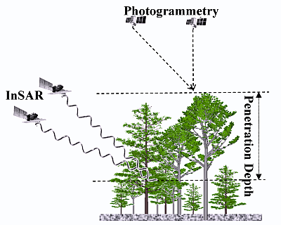
1. Introduction
Forest biomass estimation over large area and in higher accuracy becomes more and more important for the research on global climate change and carbon cycle. Synthetic Aperture Radar (SAR) has been effectively used for assessing forest biomass through the campaigns of airborne and spaceborne SARs. SAR penetrates farther into forest canopies than optical sensors, so the SAR data from forested area are primarily related to standing woody biomass, especially at longer wavelength such as L and P bands. Meanwhile, the effect of soil parameters and precipitation prior data acquisition is severe on long wavelength [1,2]. Kasischke et al. [1] found that the influence of variations in soil moisture had to be accounted in the mapping of forest biomass. Besides, the sensitivity of backscattering coefficients to forest biomass is always reduced when the biomass reaches certain level. As reported by Dobson et al. [3], the biomass saturation level for backscattering coefficients was about 200 Mg/ha at P-band and 100 Mg/ha at L-band. Therefore, the ability for forest biomass mapping by use of only the backscattering coefficients is limited. The introduction of forest canopy height in forest biomass mapping is helpful. There are five ways which could directly measure forest canopy height: (1) Lidar, which directly measures the forest canopy height using the flying time difference of lidar signals returned by forest canopy top and those by ground surface under forest [4]; (2) InSAR of two bands which employs the dependence of penetration depth of SAR data on wavelength [5]; (3) Height of scattering phase center (HSPC), which requires the elevation of ground surface under forest from other sources [6]; (4) Polarimetric Interferometric SAR (PolInSAR), which employs the dependence of penetration depth of SAR on polarization [7]; and (5) Penetration depth of SAR, which is the difference between the elevation of a forest canopy top from optical photogrammetry and that of scattering phase center from InSAR [8]. Lidar is a direct measurement of forest vertical structures and gives the most accurate estimation of the forest canopy height. However, it is difficult to collect data at regional or global scale using airborne lidar because of its cost. Spaceborne lidar such as the Geoscience Laser Altimeter System (GLAS) has already collected data globally, but only with point sampling data. Other imagery data is needed to extrapolate the samples to generate areal results. Neeff et al. [9] derived two novel digital models of vegetation height from X- and P-band interferometry separately. The difference between the surface models was called “interferometric height”. A statistical model for forest biomass as a function of both P-band backscatter and interferometric height information not only arrived at high accuracy (with R2 = 0.89 and a RMSE from cross-validation of only 46.1 t/ha), but also overcame the well-known issue of backscatter saturation. Balzter et al. [5] presented a new method for canopy height mapping using dual-wavelength SAR interferometry (InSAR) at X- and L-band. The RMSE of the dual-wavelength InSAR-derived canopy height model compared to LIDAR was 3.49 m (relative error 28.5%). Solberg et al. [10] investigated the estimation of top height, mean height of forest using interferometric X-band radar data and the ground surface elevation from airborne laser scanning data. Askne et al. [11] estimated forest biomass based on a penetration depth model using TanDEM-X data. Simard et al. [12] explored the mapping of mangrove forests height in Everglades National Park using Shuttle Radar Topography Mission (SRTM) elevation data calibrated by USGS DEM and airborne lidar data. Cloude and Papathanassiou [13] proposed the concept of PolInSAR. Then Papathanassiou and Cloude [7] examined and applied it on the estimation of forest canopy height. Cloude and Papathanassiou [14] proposed a three-stage method to improve the efficiency of the estimation of forest canopy height using PolInSAR. Garestier et al. [15] estimated Pine forest height using single-pass X-band PolInSAR data. The results showed that the associated phase centers present a significant vertical separation (about 6 m) allowed by penetration through gaps in the canopy. PolInSAR only need single frequency and no other data sources were required. It is the most promising technique for the estimation of forest height regionally or globally. However, it requires that: (1) there is negligible temporal decorrelation; (2) the wavelength is long enough to penetrate through the forest canopy. The decorrelation issues may be reduced in Tandem observations [16]. Beside Lidar, InSAR and PolInSAR, photogrammetry is another traditional technique for the extraction of digital elevation model (DEM). The information of forest canopy height should be contained in the forested area because the photogrammetry works on optical data, which is mainly reflected by top surface of the forest canopy. St-Onge et al. [17] derived the digital surface model (DSM) through photogrammetry using IKONOS stereo image. A canopy height model (CHM) was produced by subtracting the lidar DEM from the DSM. The CHM could predict above-ground biomass with a coefficient of determination of 0.79. The well known saturation point reached above 300 Mg/ha.
Among the five methods mentioned above for the estimation of forest canopy height, Lidar is only possible to be used at local scale; the method of using two bands InSAR may be possible at regional or global scale through the combination of SRTM and the InSAR data of The Phased Array type L-band Synthetic Aperture Radar (PALSAR) onboard Advanced Land Observing Satellite (ALOS) because PALSAR has systematically collected data over large areas with the aim of forming 50 m resolution global mosaic of L-band SAR data; The HSPC method is only proper for the application at country level because the digital elevation model produced by each country is always unavailable for foreigners. The PolInSAR method is limited by the accessibility of data although it holds the best promises. The penetration depth of SAR is also possible because of the global acquisition of ALOS/PALSAR data and the release of near global ASTER Global Digital Elevation Model (ASTER GDEM) which was produced by the photogrammetric processing of ASTER stereo images.
In the past, the application of stereo imageries in the estimation of forest biomass was hindered by its complicated data processing techniques. The recent development of a commercial software package makes the processing of stereo images easier. Therefore, in recent years we have been pursuing the combination of stereo imagery and InSAR data for the estimation of forest biomass because their difference should be the penetration depth of InSAR data which is direct measurements of forest vertical structures. Our previous research has demonstrated this idea based on model simulations [8]. Besides, the contributions of forest canopy height in the ASTER GDEM over forested areas has also been examined [18]. In this study, the feasibility and problems of data synthesis of PALSAR InSAR data and ASTER GDEM were investigated for the regional mapping of forest biomass from the data aspect.
2. Study Area and Dataset
2.1. Study Area
The study area is located between Bangor and Howland, Maine, USA (44.72°N–45.37°N, 68.06°W–69.08°W) as shown in Figure 1. The natural stands in this northern hardwood boreal transitional forest consist of hemlock-spruce-fir, aspen-birch, and hemlock-hardwood mixtures. The common species include Populus tremuloides (quaking aspen), Betula papyrifera (paper birch), Tsuga canadensis (eastern hemlock), Picea rubens (red spruce), Abies balsamea (balsam fir), and Acer rubrum (red maple). The region features relatively level and gently rolling topography where the elevation ranges from 28 m to 208 m within an area covered by ALOS/PALSAR data used in this study. The climate is chiefly cold, humid and continental. Summer maximum temperatures of 30 °C are common and winter minimums can reach −30 °C. The mean annual air temperature (1996–2010) at the Howland tower is 6.7 °C. Average annual rainfall (1950–2000) is 1050 mm. Precipitation is spread fairly evenly throughout the year. The growing season averages about 235 days ( http://www.nrs.fs.fed.us/ef/locations/me/howland_cef/). This site is currently used for interdisciplinary forest research and experimental forestry practices.
2.2. Dataset
2.2.1. Field Measurements
Field measurements were conducted during 2009 to 2011 by the NASA DESDynl project and a NASA supported lidar-radar fusion project. 24 plots of 1-ha (200 m × 50 m) and 10 plots of 0.5-ha (100 m × 50 m) were established in 2009 and 2010, respectively. The positions of these plots are shown in Figure 1 as yellow points. Each plot was divided into neighboring 25 m × 25 m subplots. These subplots can be aggregated into 116 subplots of 0.25-ha (50 m × 50 m). Totally, 82 subplots were selected for the model developments after removing subplots located at sparse forest. Differential Global Position System (DGPS) was used to establish the corners of these plots. For each subplot, Diameter at Breast Height (DBH, 1.3 m above ground), species, height of three highest trees, and typical tree crown information (crown width, live branch base height) in each subplot were recorded. Trees below the established size threshold (DBH > 10 cm) were counted within a 2 m transect along the center of the rectangular plot. Small stems were separated into several diameter categories. The biomass of subplots was calculated through the diameter-based allometric equations coming from the comprehensive report of USDA on North American forest given by Jenkins et al. [19]. Biomass was first calculated for each tree, and then total biomass was aggregated to subplot levels.
2.2.2. Biomass from LVIS Data
NASA’s Laser Vegetation Imaging Sensor (LVIS) is an airborne laser altimeter system designed, developed and operated by the Laser Remote Sensing Laboratory at Goddard Space Flight Center. LVIS obtained sub-canopy and canopy-top topography data as well as canopy vertical structure information for forested sites at our study area in order to generate the most detailed forest structural data sets. Blair et al [20] reported that the LVIS data used in this study acquired on June 2003 and August, 2009 with a footprint of 20 m in diameter. LVIS Ground Elevation (LGE) data were used in this study, which included location (latitude/longitude), ground surface elevation (relative to the ellipsoid WGS84), and the heights of energy quartiles (relative to surface) where 25% (RH25), 50% (RH50), 75% (RH75) and 100% (RH100) of the waveform energy occur. These quartile heights are a relatively direct measure of the vertical profile of canopy components. In addition, waveform measures are a function of the complex and variable 3-D structure of vegetation canopy components and their spectral properties including the spectral properties of the ground/litter. Drake et al. [21] reported that height of mean energy (RH50) was highly correlated with forest aboveground biomass. Their study confirmed the ability of LVIS-derived metrics to estimate biomass, even in dense tropical forests. Huang et al. [22] investigated the relationship between measured biomass of plots and LVIS metrics and found that RH50 was highly correlated with forest aboveground biomass with R2 = 0.86 and RMSE = 31.0 Mg/ha. The regressed model was
The model was applied to LVIS 2003 and 2009 LGE data. The predicted biomass was validated using the measurements of field subplots mentioned in previous section. For 0.25-ha subplots, the R2 for the relationship between predicted and measured biomass was 0.79 while the RMSE was 32.6 Mg/ha. The spatial coverage of LVIS 2009 data was shown in Figure 1 as the red polygon.
2.2.3. PALSAR InSAR Data and ASTER GDEM
The level 1.1 PALSAR data used in this study were acquired on 10 July 2007 and 25 August 2007 under dual-polarization mode (HH and HV). Their horizontal baseline component was −311.26 m while the vertical component was −90.03 m. The nominal resolutions of single look complex data were 3.53 m and 9.36 m at azimuth and range directions respectively. According to the observation at flux tower ( http://howlandforest.org/), precipitations of 5.83 mm and 21.85 cm were recorded on 5 July 2007 and 24 August 2007 respectively. The ASTER GDEM was a new global digital topographic model derived from multi-spectral imaging data collected with ASTER onboard the Terra satellite. Slater et al [23] reported that almost 1.3 million scenes of ASTER VNIR data covering the Earth land surface between 83°N and 83°S latitudes acquired from 1999 to 2010 have been processed by stereo-correlating. The ASTER GDEM was released in geotiff format with geographic lat/long coordinates and at 1 arcsecond (approximately 30 m) grid. Its latitude-longitude coordinate was referenced to the World Geodetic System 1984 (WGS 84) and the elevations were computed with respect to the EGM96 geoid. The software (GEOTRANS) developed by the National Geospatial-Intelligence Agency can calculate the differences between EGM96 geoid and theellipsoid surface of Geodetic Reference System 1980 (GRS 80). ASTER GDEM should be transformed to the ellipsoid surface of GRS80 which was the vertical reference of digital elevation model derived from PALSAR InSAR data. Besides, National Land Cover Data (NLCD) products in 2001 were used to discriminate forest and non-forest for the entire study area.
3. Method
3.1. Extraction of Penetration Depth
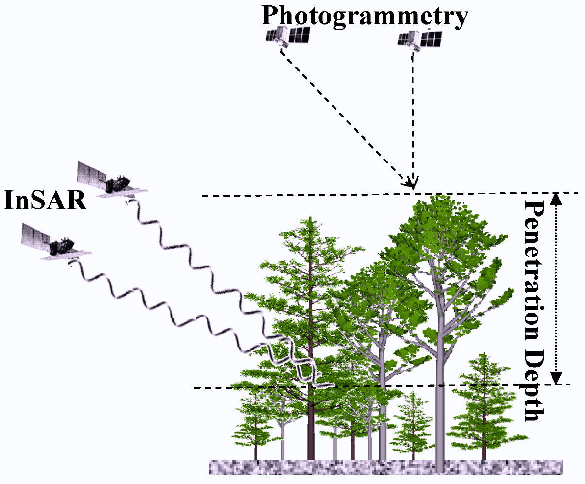
Figure 2 shows the sketch for the extraction of penetration depth through the combination of photogrammetry and InSAR techniques. Photogrammetry extracts the terrain elevation through measuring the parallax of the same ground object on the two airborne or spaceborne optical images acquired at two different positions. Interferometric SAR (InSAR) estimates the terrain elevation through measuring the distance difference from ground object to two satellites or two antennas. Photogrammetry works on optical images. The elevation estimated from photogrammetry should be that of forest canopy top surface in forested area because optical image cannot penetrate forest canopies especially in dense forest. InSAR works on microwave band. Microwave can penetrate forest canopy at a certain degree due to its long wavelength. Therefore the elevation estimated from InSAR should be lower than forest canopy top and higher than ground surface. Their difference should be the penetration depth of InSAR data.
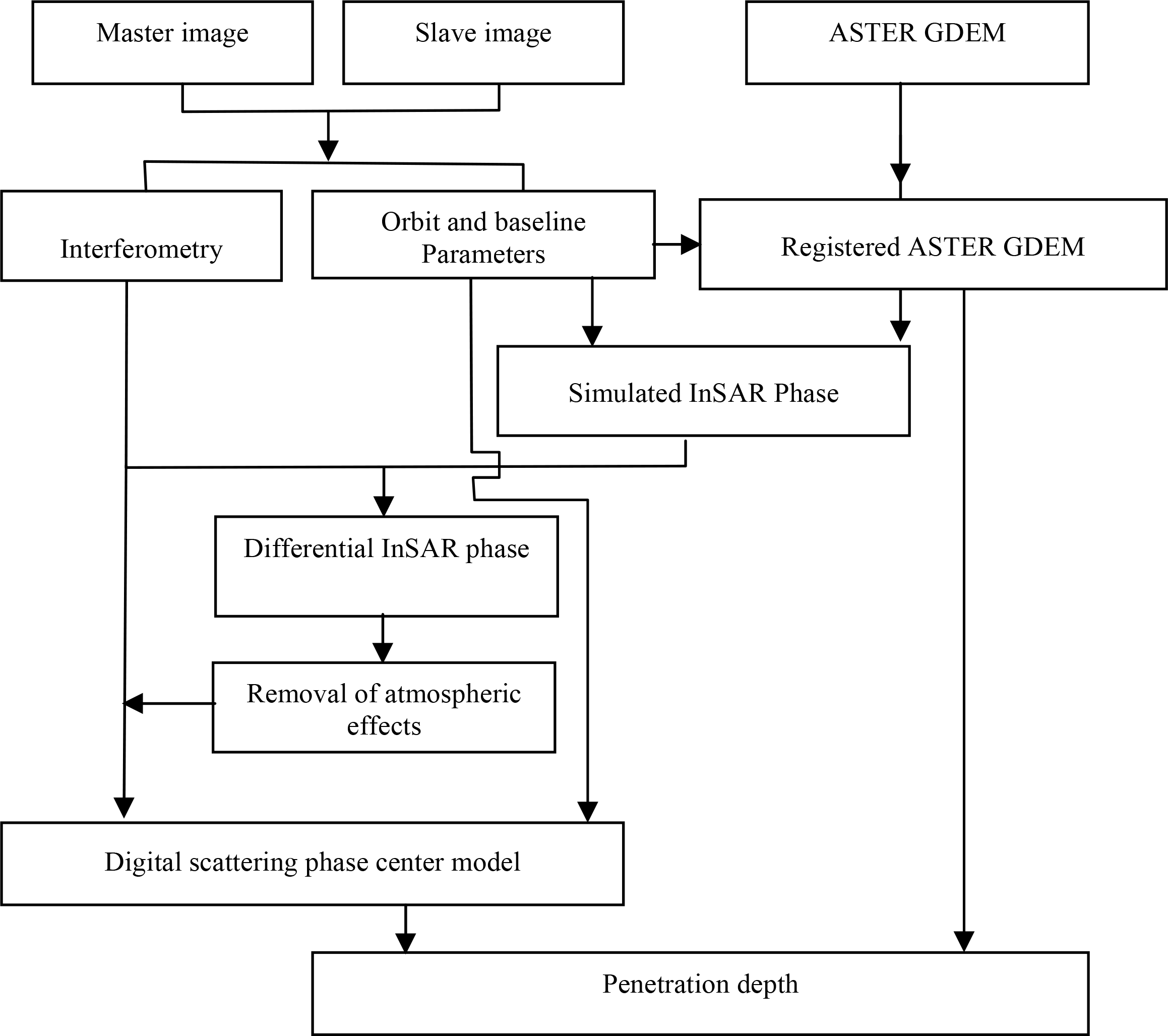
As described in previous section, ASTER GDEM was produced from the stereo-processing of ASTER images. ASTER GDEM and ALOS/PALSAR InSAR were used to extract the penetration depth. Theoretically, the direct difference between them should be the penetration depth. However, there are few factors which need to be addressed before taking the differences in practice. PALSAR InSAR data could be affected by the atmosphere. Besides, Ni et al. [24] found that the geocoding of ASTER GDEM was not accurate enough. Based on these considerations, a method for the extraction of InSAR Penetration depth was proposed and shown in Figure 3. The InSAR phase could be obtained through registration and resampling of master and slave images. Baseline parameters could be estimated from the precision orbits of InSAR image pair. ASTER GDEM was transformed into SAR slant range coordinates using orbit and baseline parameters, and was further registered to the amplitude image of InSAR to generate simulated InSAR phase. The atmospheric effects on InSAR data can be recognized in the differential InSAR phase data using the method developed by Ni et al. [25]. The Digital Scattering Phase Center Model (DSPCM) could be produced after the atmospheric effect was removed from InSAR phase. Finally, the penetration depth was obtained from the difference between DSPCM and Registered ASTER GDEM.
3.2. Biomass Estimation and Assessments
Three models using different independent variables for the forest biomass estimation were built: (1) model only using backscattering coefficients; (2) model only using penetration depth; and (3) model from the combination of backscattering coefficients and the penetration depth. For simplicity, they were referred to as model I, model II and model III in following sections. The models were built on the 0.25-ha subplot measurements. The independent variables were selected from backscattering coefficients or/and penetration depth of HH and HV polarization through the stepwise regression method. Then they were applied on the whole scene of PALSAR InSAR data. The results were evaluated using the biomass from LVIS data acquired in 2009 at different scales (60 m, 90 m, 120 m and 510 m) to assess the scale effects. As mentioned in previous sections, ASTER GDEM was produced using the ASTER images acquired between 1999 and 2010, therefore the forest changes, especially the forest disturbance had to be considered. In this study, the difference of biomass map from LVIS 2009 and 2003 data were used to identify the forest disturbance. The pixels which had negative values were excluded in the model assessments. Ni et al. [18] found that the spatial homogeneity of forest stands could affect the correlation between forest height derived from the difference of ASTER GDEM and NED and LVIS energy quartiles. The spatial homogeneity in this study was defined by the standard deviation of penetration depth of the given pixel size calculated from 30 m sub-pixel size. For example, the spatial homogeneity of data at 60 m pixel size was defined by the standard deviation of penetration depth of the corresponding 4 pixels of 30m while that of 90 m was defined by the standard deviation of penetration depth of the corresponding 9 pixels of 30 m. Six cases were considered for each model at each resolution (1) forest disturbance and spatial homogeneity are not considered; (2) forest disturbance is considered; (3) both the forest disturbance and spatial homogeneity were considered while the spatial homogeneity were defined by the standard deviation smaller than 5 m, 4 m, 3 m and 2 m separately.
4. Results
4.1. Penetration Depth
Figure 4 shows the quality of InSAR data and penetration depth from ASTER GDEM and PALSAR InSAR (HV polarization). Coherence which is the correlation between two SAR images within given window size is an important parameter to measure the quality of repeat-pass InSAR data. Figure 4a is the coherence map of InSAR data. For most area, the coherence is higher than 0.5. Figure 4b is the differential InSAR phase derived by ASTER GDEM and PALSAR InSAR data. It can be seen that there is low spatial frequency blue-red pattern in addition to the high frequency features related to ground objects. The low frequency pattern should be from the atmospheric effects. Figure 4c is the atmospheric effect recognized by the step-wise spatial filtering method developed by Ni et al. [25]. Figure 4d is the penetration depth map after the atmospheric effect is removed. It is clear that the atmospheric effect has been successfully removed.
4.2. Biomass Mapping
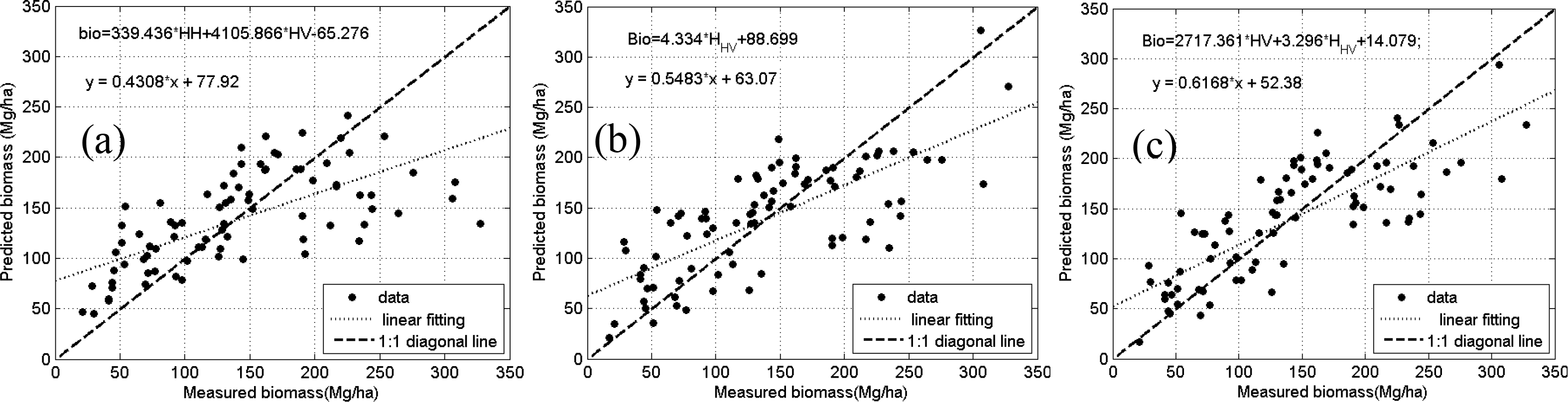
Table 1 shows the three biomass estimation models using field measurements at 0.25-ha plots selected by stepwise regression methods. The first column is the input variables. σHH, σHV are the backscattering coefficients while HHH, HHV are the penetration depth at HH and HV polarizations, respectively. The second column is the estimation models of forest biomass derived by stepwise regression. The third column is the evaluation results of selected models. “Linear fitting” shows the equation derived by linear fitting between the measured and estimated biomass of subplots. “R2” and “RMSE” are the evaluation about the linear fitting equations. It can be seen that both HH and HV polarizations of backscattering coefficients have contributions on biomass estimation while only HV polarization is remained when the penetration depth is employed. The penetration depth performed better than backscattering coefficients because R2 increased from 0.44 to 0.55 while RMSE was reduced from 56.68 to 50.47 Mg/ha. The combination of backscattering coefficients and penetration depth gives the highest estimation accuracy with R2 = 0.62 and RMSE = 46.60 Mg/ha. Figure 5 shows the scatter plots corresponding to Table 1. The effect of penetration depth in the estimation of forest biomass is obvious. Figure 5a shows that the saturation point appeared between 150 Mg/ha and 200 Mg/ha. Figure 5b shows the penetration depth still correlated with forest biomass over 300 Mg/ha although a set of plots from 200 Mg/h to 250 Mg/h are underestimated. Figure 5c shows that the underestimated subplots in Figure 5a and Figure 5b are improved through the combination of backscattering coefficients and penetration depth.
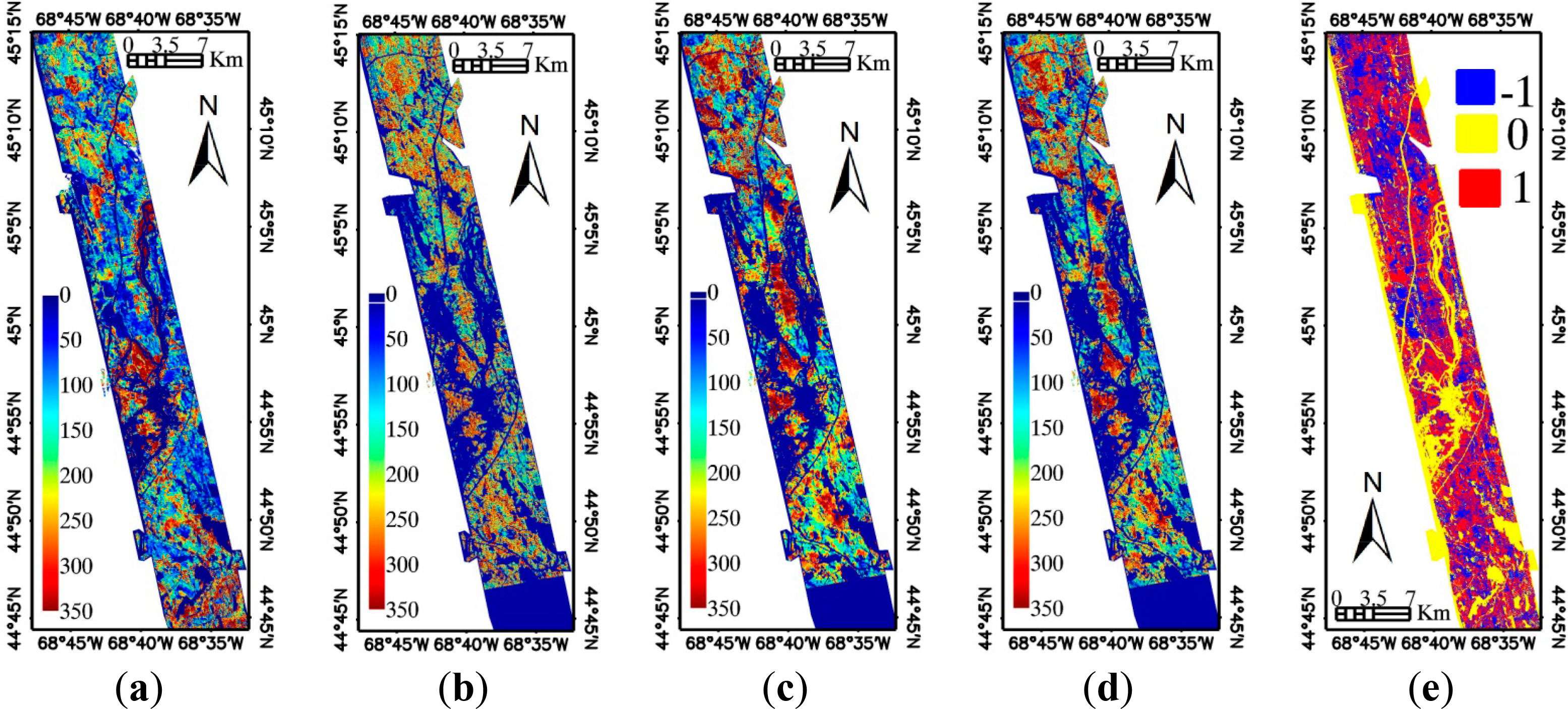
Figure 6 shows the biomass maps from different models over the commonly covered areas by LVIS and PALSAR InSAR data. Figure 6e is the forest change recognized from LVIS 2009 and LVIS 2003 data. −1 stands for forest disturbance. It is clear that the most obvious disagreement between biomass from LVIS 2009 and that from SAR data mainly occurred over the disturbance area.
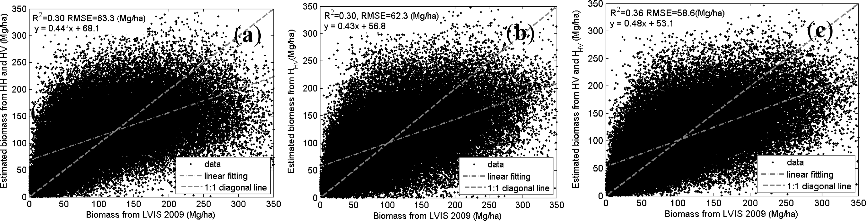
Figure 7 is the scatter plots of forest biomass from LVIS 2009 against those from different models. The forest disturbance areas are not excluded. The Y axis of Figure 7a, Figure 7b and Figure 7c correspond to biomass values in Figure 6b, Figure 6c and Figure 6d. It can be seen that the overall accuracy of biomass estimation from penetration depth approximately the same with that from backscattering coefficients. Their combination works a little better than both of them.
Table 2 is the effects of spatial resolution and forest homogeneity on the validation of models. The first column indicates the pixel size used in the model validation. The resolutions used here are integer times of 30 m to minimize the error introduced in data resampling. The pixel value of each resolution is a direct average of the corresponding pixels in 30 m. The second column indicates forest spatial homogeneity. “all” means the entire area was used in the validation without consideration of forest disturbance. “undisturbed” means the area of forest disturbance is excluded in model validation. The map of forest disturbance (Figure 6e) is recalculated for each resolution from forest biomass change which is calculated in the same way as biomass map at the same resolution. The pixels having negative values of biomass difference are excluded in the validation. “5”, “4”, “3”, “2” are used to define the forest spatial homogeneity. For example, the “5” means that the pixels whose standard deviation of penetration depth calculated from 30 m sub-pixels is less than 5 m are used in model validation. The results from different biomass estimation models are listed in the Table 2. “Equation”, “R2” and “RMSE” under each model are used to describe the correlation between the biomass from LVIS 2009 data and that estimated from the corresponding model using linear regression over their scatter plots.
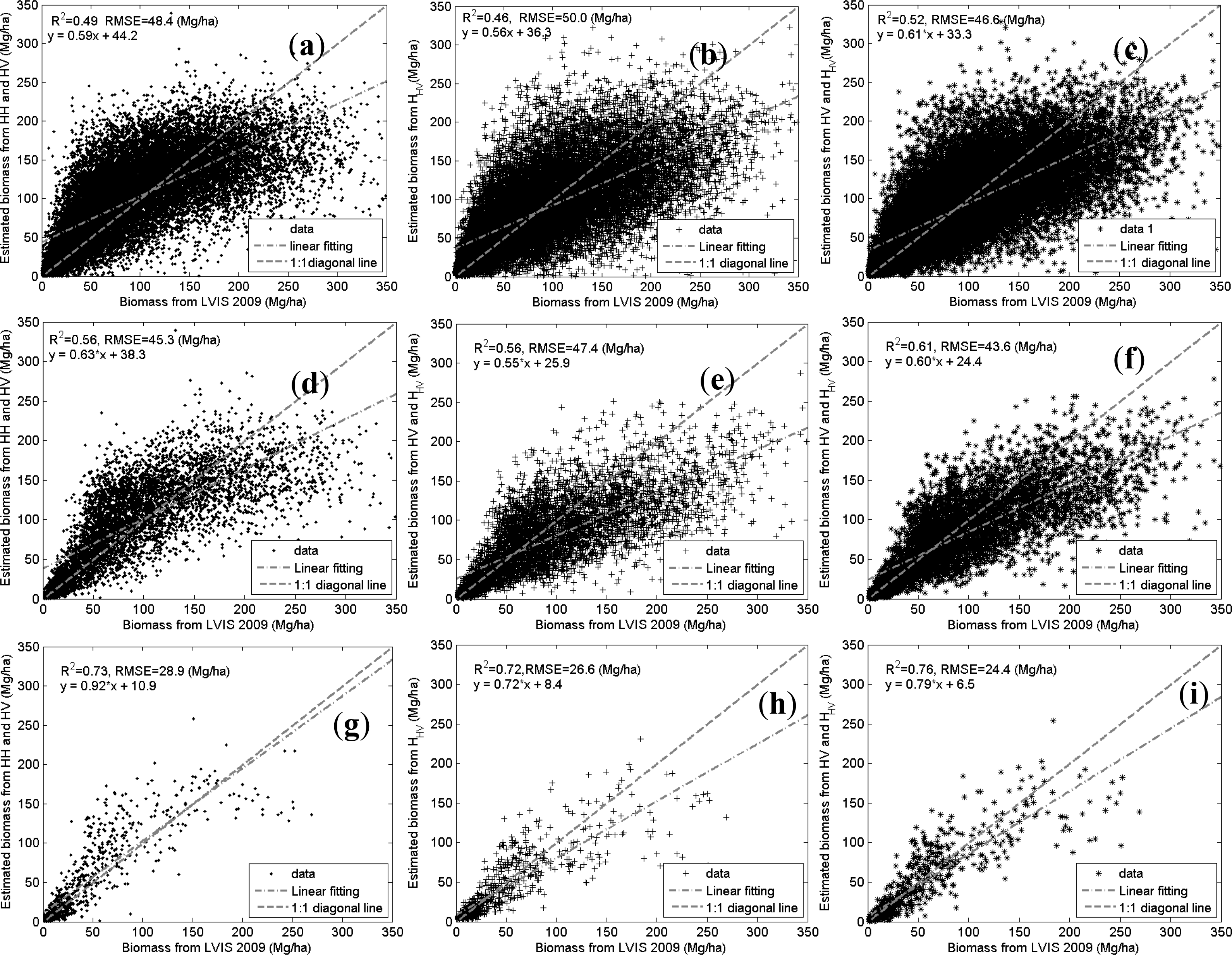
Table 2 is also expressed graphically as shown in Figure 8. The y axis in Figure 8a and Figure 8b is R2 and RMSE of Table 2, respectively. The x axis in Figure 8 is cases with different spatial homogeneities. Plus, star and triangle stands for the results from model I, model II and model III, respectively. Solid line, dash line, dot line and dash-dot line are corresponding to the results of 60 m, 90 m, 120 m and 510 m, respectively. Figure 9 shows the scatter plot of the case on 120 m resolution. The forest disturbance was not excluded in the first row of Figure 9 (Figure 9a–c). The forest disturbance and spatial homogeneity of 5 m are applied on the second row of Figure 9 (Figure 9d–f). The forest disturbance and spatial homogeneity of 2 m are applied on the last row of Figure 9 (Figure 9g–i).
It is clear that R2 increases while RMSE decreases along with the increase of pixel size. The effect of spatial homogeneity on high resolution results is weaker than that on low resolution results. As shown in Figure 8, the R2 of low resolution results goes up while RMSE goes down along with the requirement of spatial homogeneity becomes stricter. The introduction of penetration depth has great impact on high resolution results, especially after the forest disturbance area was excluded. Taking the 60 m case as an example, the R2 of model I is about 0.29–0.30 while that of model II is about 0.39–0.40. Model III shows the highest accuracy with R2 = 0.43 –0.44 while RMSE = 58.9 Mg/ha ∼55.9 Mg/ha. For low resolution results, the accuracy of model II is high although it is lower than that of model I.
5. Discussion
The results show that forest disturbance has important impacts on the estimation of forest biomass when the penetration depth is employed. This should be attributed to the long time span of ASTER GDEM. In ASTER GDEM processing, multiple temporal observations were used to improve the data quality, but there was a balance between time span of ASTER GDEM and data quality. The quality of photogrammetry mainly depends on the common points recognized in the stereo-image pair. The recognition of common points could be affected by the observation geometry as while as the tree conditions. Over certain areas, common points may be identified in some stereo-image pairs but not in others acquired under different geometry or at different seasons. The long time span is useful for the improvement of data quality through the average of more stereo-image pairs. However, if the time span is so long that forest disturbance occurred, the data quality would be degraded in terms of the information of forest canopy height. Therefore, it is necessary to investigate the characteristics of common points that can be recognized in forest area and to explore if there is a principle for the improvement of data quality using extended time span. As to ASTER GDEM, it is recommended to deliver the time span of each pixel along with the data. It would be helpful for user to consider the forest disturbance.
Besides ASTER GDEM, the quality of PALSAR InSAR data is also very important if the penetration depth is employed to estimate forest biomass. This study mainly focused on the feasibility of forest biomass estimation using penetration depth. The influence of InSAR data quality on forest biomass estimation will be quantitatively investigated in future research.
The results show that the forest spatial homogeneity can also affect the estimation accuracy. This may be due to the common points recognized in forest area. For heterogeneous or spars forest, the common points recognized from different stereo-image pair will vary because the visible part of tree will be different for different observation geometry. Another reason may be that some filtering process has been applied to remove forest information in the generation of ASTER GDEM because the main aim of ASTER GDEM is to provide the elevation of ground surface. Filtering method should be more effective at sparse forest because the ground surface can be relatively easily found at given widow size than homogenous forest. If that is the case, it is suggested to release a version of ASTER GDEM without filtering.
In this study, for convenience, the forest disturbance is identified using the change of biomass from LVIS data. It may be either longer or shorter than that of ASTER GDEM. We cannot exactly exclude the forest disturbance because of the lack of information about time span of ASTER GDEM over the test site. If the time span is provided, the forest disturbance can be recognized by optical data such as Landsat image at high resolution (30 m or 60 m) and MODIS data at low resolution (500 m).
6. Conclusions
The spatial distribution of forest biomass is critical for research into the global carbon cycle or climate changes. Synthetic Aperture Radar (SAR) is a useful tool for the regional mapping of forest biomass because of its large spatial coverage and its penetration ability. The accuracy of forest biomass estimation based on the SAR backscattering coefficients is limited because backscattering coefficients are also affected by environmental factors, such as soil roughness and soil moistures. The information of forest vertical structures will be helpful to improve the estimation accuracy of forest biomass. In this study, the concept of penetration depth was proposed based on the synthesis of a digital surface model from stereo images (ASTER GDEM) and interferometric SAR (ALOS/PALSAR) data. A procedure for the derivation of penetration depth was developed. Then the feasibility of forest biomass estimation through the data synthesis of backscatering coefficients and penetration depth was explored. The results showed that introduction of penetration depth could clearly improve the accuracy of forest biomass estimation. The correlation (R2) between the predicted biomass and the field measurement over sampling plots was improved from 0.44 to 0.62. The forest disturbance had to be considered in the application of the penetration depth algorithm because of the long time span (from 1999 to 2010) of ASTER data used to generate GDEM. Forest spatial homogeneity was another important aspect which should be considered in the forest biomass estimation using penetration depth. This study mainly demonstrated the possibility of forest biomass estimation with the help of the penetration depth from the data aspect. There are still many issues that need to be explored in our future research before it becomes a practical method, including the effects of forest disturbance, the temporal decorrelation and so on.
Acknowledgments
This work was supported in part by the National Basic Research Program of China (Grant No. 2013CB733404), the National Natural Science Foundation of China (Grant No. 41371357, 41001208, 40971203, 41171283). The PALSAR data were provided by JAXA. Authors would like to give thanks to them.
Author Contributions
Zhiyu Zhang and Guoqing Sun recorded the field data. Wenjian Ni processed ASTER GDEM and PALSAR data for the extraction of penetration depth and wrote the paper. Guoqing Sun contributed important ideas and considerations. Results and text were discussed Zhifeng Guo and Yating He.
Conflicts of Interest
The authors declare no conflict of interest.
References
- Kasischke, E.S.; Tanase, M.A.; Bourgeau-Chavez, L.L.; Borr, M. Soil moisture limitations on monitoring boreal forest regrowth using spaceborne L-band SAR data. Remote Sens. Environ 2011, 115, 227–232. [Google Scholar]
- Liesenberg, V.; Gloaguen, R. Evaluating SAR polarization modes at L-band for forest classification purposes in Eastern Amazon, Brazil. Int. J. Appl. Earth Obs. Geoinf 2013, 21, 122–135. [Google Scholar]
- Dobson, M.C.; Ulaby, F.T.; LeToan, T.; Beaudoin, A.; Kasischke, E.S.; Christensen, N. Dependence of radar backscatter on coniferous forest biomass. IEEE Trans. Geosci. Remote Sens 1992, 30, 412–415. [Google Scholar]
- Sun, G.; Ranson, K.J.; Guo, Z.; Zhang, Z.; Montesano, P.; Kimes, D. Forest biomass mapping from lidar and radar synergies. Remote Sens. Environ 2011, 115, 2906–2916. [Google Scholar]
- Balzter, H.; Rowland, C.S.; Saich, P. Forest canopy height and carbon estimation at Monks Wood National Nature Reserve, UK, using dual-wavelength SAR interferometry. Remote Sens. Environ 2007, 108, 224–239. [Google Scholar]
- Kellndorfer, J.; Walker, W.; Pierce, L.; Dobson, C.; Fites, J.A.; Hunsaker, C.; Vona, J.; Clutter, M. Vegetation height estimation from shuttle radar topography mission and national elevation datasets. Remote Sens. Environ 2004, 93, 339–358. [Google Scholar]
- Papathanassiou, K.P.; Cloude, S.R. Single-baseline polarimetric SAR interferometry. IEEE Trans. Geosci. Remote Sens 2001, 39, 2352–2363. [Google Scholar]
- Ni, W.; Sun, G.; Ranson, K.J.; Zhang, Z.; Guo, Z.; Huang, W. Model based analysis of the influence of forest structures on the scattering phase center at L-band. IEEE Trans. Geosci. Remote Sens 2014, 52, 3937–3946. [Google Scholar]
- Neeff, T.; Dutra, L.V.; dos Santos, J.R.; Freitas, C.D.; Araujo, L.S. Tropical forest measurement by interferometric height modeling and P-band radar backscatter. Forest Sci 2005, 51, 585–594. [Google Scholar]
- Solberg, S.; Astrup, R.; Gobakken, T.; Naesset, E.; Weydahl, D.J. Estimating spruce and pine biomass with interferometric X-band SAR. Remote Sens. Environ 2010, 114, 2353–2360. [Google Scholar]
- Askne, J.I.H.; Fransson, J.E.S.; Santoro, M.; Soja, M.J.; Ulander, L.M.H. Model-Based biomass estimation of a Hemi-Boreal forest from multitemporal TanDEM-X acquisitions. Remote Sens 2013, 5, 5574–5597. [Google Scholar]
- Simard, M.; Zhang, K.Q.; Rivera-Monroy, V.H.; Ross, M.S.; Ruiz, P.L.; Castaneda-Moya, E.; Twilley, R.R.; Rodriguez, E. Mapping height and biomass of mangrove forests in Everglades National Park with SRTM elevation data. Photogramm. Eng. Remote Sens 2006, 72, 299–311. [Google Scholar]
- Cloude, S.R.; Papathanassiou, K.P. Polarimetric SAR interferometry. IEEE Trans. Geosci. Remote Sens 1998, 36, 1551–1565. [Google Scholar]
- Cloude, S.R.; Papathanassiou, K.P. Three-stage inversion process for polarimetric SAR interferometry. IEE Proc. Radar Sonar Navig 2003, 150, 125–134. [Google Scholar]
- Garestier, F.; Dubois-Fernandez, P.C.; Papathanassiou, K.P. Pine forest height inversion using single-pass X-band Polinsar data. IEEE Trans. Geosci. Remote Sens 2008, 46, 59–68. [Google Scholar]
- Kugler, F.; Schulze, D.; Hajnsek, I.; Pretzsch, H.; Papathanassiou, K.P. TanDEM-X Pol-InSAR performance for forest height estimation. IEEE Trans. Geosci. Remote Sens 2014, 52, 6404–6422. [Google Scholar]
- St-Onge, B.; Hu, Y.; Vega, C. Mapping the height and above-ground biomass of a mixed forest using lidar and stereo Ikonos images. Int. J. Remote Sens 2008, 29, 1277–1294. [Google Scholar]
- Ni, W.; Sun, G.; Ranson, K.J. Characterization of ASTER GDEM elevation data over vegetated area compared with lidar data. Int. J. Digital Earth 2013. [CrossRef]
- Jenkins, J.C.; Chojnacky, D.C.; Heath, L.S.; Birdsey, R.A. National-scale biomass estimators for United States tree species. For. Sci 2003, 49, 12–35. [Google Scholar]
- Blair, J.B.; Hofton, M.A.; Rabine, D.L. Processing of NASA LVIS Elevation and Canopy (LGE, LCE and LGW) Data Products, Version 1.0, Available online: http://lvis.gsfc.nasa.gov (accessed on 21 July 2014).
- Drake, J.; Dubayah, R.; Clark, D.; Knox, R.; Blair, J.; Hofton, M.; Chazdon, R.; Weishampel, J.; Prince, S. Estimation of tropical forest structural characteristics using large-footprint lidar. Remote Sens. Environ 2002, 79, 305–319. [Google Scholar]
- Huang, W.L.; Sun, G.Q.; Dubayah, R.; Cook, B.; Montesano, P.; Ni, W.J.; Zhang, Z.Y. Mapping biomass change after forest disturbance: Applying LiDAR footprint-derived models at key map scales. Remote Sens. Environ 2013, 134, 319–332. [Google Scholar]
- Slater, J.A.; Heady, B.; Kroenung, G.; Curtis, W.; Haase, J.; Hoegemann, D.; Shockley, C.; Tracy, K. Evaluation of the New ASTER Global Digital Elevation Model; National Geospatial-Intelligence Agency: Springfield, VA, USA, 2009. [Google Scholar]
- Ni, W.; Guo, Z.; Sun, G.; Chi, H. Investigation of forest height retrieval using SRTM-DEM and ASTER-GDEM. Proceedings of 2010 IEEE International Geoscience and Remote Sensing Symposium, Honululu, HI, USA, 25–30 July 2010; pp. 2111–2114.
- Ni, W.; Sun, G.; Zhang, Z.; Guo, Z.; He, Y. A heuristic approach to reduce atmospheric effects in InSAR data for the derivation of digital terrain models or for the characterization of forest vertical structure. IEEE Geosci. Remote Sens. Lett 2014, 11, 268–272. [Google Scholar]


| Input Variables | Selected Model | Model Evaluation | ||
|---|---|---|---|---|
| Linear Fitting | R2 | RMSE (Mg/ha) | ||
| σHH, σHV | Bio = 339.436 × σHH + 4105.866 × σHV − 65.276 | y = 0.4308 × x + 77.92 | 0.44 | 56.68 |
| HHH, HHV | Bio = 4.334 HHV + 88.699 | y = 0.5483 × x + 63.07 | 0.55 | 50.47 |
| σHH, σHV, HHH, HHV | Bio = 2717.361 σHV + 3.296 HHV + 14.079 | y = 0.6168 × x + 52.38 | 0.62 | 46.60 |
| Resolution | Spatial Homogeneity | Models | ||||||||
|---|---|---|---|---|---|---|---|---|---|---|
| Model I | Model II | Model III | ||||||||
| Equation | R2 | RMSE | Equation | R2 | RMSE | Equation | R2 | RMSE | ||
| 60 m | all | y = 0.44x + 68.1 | 0.30 | 63.3 | y = 0.43x + 56.8 | 0.30 | 62.3 | y = 0.48x + 53.1 | 0.36 | 58.6 |
| undisturbed | y = 0.44x + 65.4 | 0.30 | 63.6 | y = 0.46x + 45.4 | 0.36 | 64.1 | y = 0.50x + 44.3 | 0.42 | 60.1 | |
| 5 | y = 0.43x + 68.8 | 0.29 | 63.6 | y = 0.45x + 45.3 | 0.38 | 62.6 | y = 0.48x + 44.5 | 0.43 | 58.9 | |
| 4 | y = 0.42x + 69.9 | 0.29 | 63.8 | y = 0.44x + 46.0 | 0.38 | 62.3 | y = 0.48x + 45.2 | 0.43 | 58.6 | |
| 3 | y = 0.43x + 70.1 | 0.29 | 63.4 | y = 0.44x + 46.2 | 0.39 | 61.2 | y = 0.48x + 45.4 | 0.43 | 57.6 | |
| 2 | y = 0.45x + 68.2 | 0.30 | 62.6 | y = 0.44x + 45.7 | 0.39 | 59.4 | y = 0.49x + 44.5 | 0.44 | 55.9 | |
| 90 m | all | y = 0.54x + 52.4 | 0.43 | 53.9 | y = 0.52x + 43.4 | 0.40 | 54.8 | y = 0.56x + 40.1 | 0.47 | 51.1 |
| undisturbed | y = 0.52x+50.6 | 0.44 | 54.3 | y = 0.52x + 35.1 | 0.45 | 57.1 | y = 0.56x + 33.8 | 0.51 | 52.9 | |
| 5 | y = 0.55x+49.6 | 0.46 | 52.3 | y = 0.52x+32.4 | 0.50 | 53.7 | y = 0.56x + 31.2 | 0.55 | 49.6 | |
| 4 | y = 0.57x + 47.9 | 0.48 | 51.7 | y = 0.52x+31.5 | 0.51 | 52.4 | y = 0.57x + 30.2 | 0.57 | 48.4 | |
| 3 | y = 0.61x+43.5 | 0.51 | 49.8 | y = 0.54x + 49.2 | 0.54 | 49.2 | y = 0.59 + 27.9 | 0.59 | 45.5 | |
| 2 | y = 0.73x + 33.6 | 0.55 | 47.7 | y = 0.6x + 26.3 | 0.56 | 41.5 | y = 0.67x + 23.8 | 0.61 | 39.5 | |
| 120 m | all | y = 0.59x+44.2 | 0.49 | 48.4 | y = 0.56x + 36.3 | 0.46 | 50.0 | y = 0.61x + 33.3 | 0.52 | 46.6 |
| undisturbed | y = 0.56x + 42.7 | 0.51 | 49.1 | y = 0.55x + 29.8 | 0.50 | 52.7 | y = 0.59x + 28.4 | 0.56 | 48.8 | |
| 5 | y = 0.63x + 38.3 | 0.56 | 45.3 | y = 0.55x + 25.9 | 0.56 | 47.4 | y = 0.60x + 24.4 | 0.61 | 43.6 | |
| 4 | y = 0.67x+34.5 | 0.59 | 43.3 | y = 0.55x + 24.5 | 0.58 | 45.4 | y = 0.61x + 22.9 | 0.63 | 41.5 | |
| 3 | y = 0.73x + 27.9 | 0.62 | 41.2 | y = 0.58x + 20.0 | 0.63 | 40.7 | y = 0.65x + 18.7 | 0.66 | 37.8 | |
| 2 | y = 0.92x + 10.9 | 0.73 | 28.9 | y = 0.72x + 8.4 | 0.72 | 26.6 | y = 0.79x + 6.5 | 0.76 | 24.4 | |
| 510 m | all | y = 0.79x + 19.1 | 0.69 | 29.1 | y = 0.71x + 16.5 | 0.62 | 32.1 | y = 0.75x + 14.3 | 0.67 | 29.8 |
| undisturbed | y = 0.74x + 18.3 | 0.69 | 29.0 | y = 0.67x + 14.55 | 0.64 | 33.2 | y = 0.72x + 12.4 | 0.69 | 30.5 | |
| 5 | y = 0.94x+8.5 | 0.77 | 20.65 | y = 0.67x + 8.99 | 0.69 | 22.2 | y = 0.75x + 6.9 | 0.76 | 19.5 | |
| 4 | y = 1.25x − 0.04 | 0.76 | 17.6 | y = 0.84x + 2.5 | 0.72 | 12.3 | y = 0.92x + 1.4 | 0.75 | 11.9 | |
| 3 | y = 1.45x − 3.5 | 0.86 | 9.9 | y = 0.95x − 0.3 | 0.81 | 6.0 | y = 1.05x − 1.5 | 0.84 | 6.0 | |
| 2 | y = 1.05x − 0.6 | 0.82 | 2.3 | y = 0.86x − 0.5 | 0.82 | 2.2 | y = 0.84x − 0.5 | 0.82 | 2.3 | |
© 2014 by the authors; licensee MDPI, Basel, Switzerland This article is an open access article distributed under the terms and conditions of the Creative Commons Attribution license (http://creativecommons.org/licenses/by/3.0/).
Share and Cite
Ni, W.; Zhang, Z.; Sun, G.; Guo, Z.; He, Y. The Penetration Depth Derived from the Synthesis of ALOS/PALSAR InSAR Data and ASTER GDEM for the Mapping of Forest Biomass. Remote Sens. 2014, 6, 7303-7319. https://doi.org/10.3390/rs6087303
Ni W, Zhang Z, Sun G, Guo Z, He Y. The Penetration Depth Derived from the Synthesis of ALOS/PALSAR InSAR Data and ASTER GDEM for the Mapping of Forest Biomass. Remote Sensing. 2014; 6(8):7303-7319. https://doi.org/10.3390/rs6087303
Chicago/Turabian StyleNi, Wenjian, Zhiyu Zhang, Guoqing Sun, Zhifeng Guo, and Yating He. 2014. "The Penetration Depth Derived from the Synthesis of ALOS/PALSAR InSAR Data and ASTER GDEM for the Mapping of Forest Biomass" Remote Sensing 6, no. 8: 7303-7319. https://doi.org/10.3390/rs6087303