Structural Changes of Desertified and Managed Shrubland Landscapes in Response to Drought: Spectral, Spatial and Temporal Analyses

Abstract

Drought events cause changes in ecosystem function and structure by reducing the shrub abundance and expanding the biological soil crusts (biocrusts). This change increases the leakage of nutrient resources and water into the river streams in semi-arid areas. A common management solution for decreasing this loss of resources is to create a runoff-harvesting system (RHS). The objective of the current research is to apply geo-information techniques, including remote sensing and geographic information systems (GIS), on the watershed scale, to monitor and analyze the spatial and temporal changes in response to drought of two source-sink systems, the natural shrubland and the human-made RHSs in the semi-arid area of the northern Negev Desert, Israel. This was done by evaluating the changes in soil, vegetation and landscape cover. The spatial changes were evaluated by three spectral indices: Normalized Difference Vegetation Index (NDVI), Crust Index (CI) and landscape classification change between 2003 and 2010. In addition, we examined the effects of environmental factors on NDVI, CI and their clustering after successive drought years. The results show that vegetation cover indicates a negative ΔNDVI change due to a reduction in the abundance of woody vegetation. On the other hand, the soil cover change data indicate a positive ΔCI change due to the expansion of the biocrusts. These two trends are evidence for degradation processes in terms of resource conservation and bio-production. A considerable part of the changed area (39%) represents transitions between redistribution processes of resources, such as water, sediments, nutrients and seeds, on the watershed scale. In the pre-drought period, resource redistribution mainly occurred on the slope scale, while in the post-drought period, resource redistribution occurred on the whole watershed scale. However, the RHS management is effective in reducing leakage, since these systems are located on the slopes where the magnitude of runoff pulses is low.

1. Introduction

Shrublands in arid and semi-arid areas, on a small spatial scale, are characterized by a structure of a “two-phase landscape mosaic” of woody vegetated patches and bare or soil-crusted patches [1]. Water, sediments, nutrients and seeds flow across the system, between the components of the landscape mosaic, creating a functional “sink-source” relationship. The crusted soil matrix is the contributory source [2], while the scattered shrub patches act as sinks, capturing the fluxes of the abiotic and biotic elements [3–7]. The spatial variation of the two-phase mosaic in the landscape regulates the water flow and can be considered hydro-ecosystem engineering [8–11].

In the last few decades, a rise in temperature, more frequent drought events and changes in the precipitation regime in arid and semi-arid areas have been observed and reported [12,13]. A number of climate models predict that desertification of many drylands worldwide will occur [14–17]. This focuses the attention of many researchers on the relationships between climate change and desertification in the semi-arid areas that are located in the transition zones between deserts and arable land, due to their high susceptibility to degradation [18]. The change in aridity poses a threat to ecosystems in these areas by altering landscape structure and function. On the one hand, a decrease in precipitation and higher temperatures are drivers of woody vegetation mortality [19–22], and on the other hand, stronger rainfall intensities increase the susceptibility of soil to erosion and flash floods [23]. These changes disturb the function of the present ecosystem source-sink relationship by reducing the shrub cover, which decreases the sink function, resulting in a reduction in resource conservation and an expansion of the biocrust areas that increase the source function of that system, resulting in the leakage of resources [24–26]. In addition to climatic changes, the shrublands in arid and semi-arid areas have been exposed to human activities for thousands of years. Land-use practices, such as livestock grazing and clear cutting, cause a reduction in the abundance of shrub patches and an increase in the biological soil crust cover [27]. Both climate and land-use changes reduce the sink function of the landscape, resulting in the resource leakage of water, organic matter and nutrients and, consequently, in low ecosystem productivity and biodiversity [4,11,25].

On the watershed scale, the relationship between shrub abundance (sink patches) on the slope and river stream flow is based on the spatial configuration of runoff production: crust-covered areas (sources) and runoff-absorbing areas with woody vegetation, plant litter and depressions (sinks) in the watershed slopes [4,7]. While rainfall absorption and runoff production take place at the small scale, due to differences in water infiltration in the sinks and sources [4,25,28], the magnitude and frequency of runoff flow on the slopes and into the river streams depend on the size and location of the source and sink areas, relative to each other. In the arid lands of Israel, where the shrub patches play a major role in the productivity and stability of the ecosystem as fertility islands, the reduction of sink patches makes the entire ecosystem vulnerable to degradation. Degraded arid lands tend to suffer from leakages of resources and water into nearby river streams, due to the system’s inability to retain them by physical or biological means [11,29,30].

A common management solution for decreasing the loss of resources in semi-arid areas is to create human-made arrays of source and sink patches [31]. These arrays have a contoured shape, 10–15 m between the contour dikes, usually following the topographic contour [11,25]. These human-made mosaics are termed “contour line mini-catchments”. Each mini-catchment has three parts. The first is the gently sloped area covered mainly by biocrusts that function as a source of runoff, soil, organic matter and nutrients to the second part. The second is an elongated pit that absorbs and stores these resources, forming resource-enriched patches. The third includes one meter-high soil mounds that prevent the flow of the resources out of the mini-catchment. These contour catchments, termed “runoff-harvesting system” (RHS), spatially integrate natural and human-made arrays in order to harvest runoff water and their associated resources from the natural source area and to concentrate them in the water-enriched zones, where trees are planted and grow together with natural understory vegetation [11]. In Israel, RHSs were constructed along the desert fringe in an attempt to combat desertification and rehabilitate degraded shrubland. Adding human-made sink patches to the system alters the distribution of the abovementioned resources, modifies the landscape connectivity and stability and increases the productivity and diversity of desertified areas [32].

Changes in the configuration of runoff-producing areas (sources) and runoff-absorbing areas and depressions (sinks) in semi-arid regions were found to be essential for the eco-hydrology management of degraded lands [33,34]. Consequently, relatively large areas (about 5000 ha) in the northern Negev Desert have been changed during the last few decades from desertified shrublands to RHSs by the Forest Department of the Jewish National Fund (JNF) [11]. This initiative is called “savannization”, since trees are successfully grown in the sink patches, and the former degraded areas are now characterized by a planted-forest landscape with herbaceous vegetation as the understory, mainly in the human-made pits. The management is based on the idea that the production and diversity in desertified shrublands is not limited by a lack of resources, but by their spatial distribution. It has been proposed that existing water and nutrient resources are not used by biotic elements, because they leak from the landscape before they are concentrated in water-enriched patches and are able to be used by vegetation, animals and humans [35,36].

Recent studies emphasized the importance of changes in vegetation and soil cover as indicators for identifying the changes in the extent, distribution and connectivity of runoff and sediment (e.g., [3,37,38]). These changes determine the movement of abiotic and biotic elements across the landscape and their concentration in resource-enriched patches. The movement and the concentration of the elements among patches from a source area to a sink area are the main drivers of the ecosystem dynamics and are defined as the “source and sink relations” among patches that create resource-deprived and resource-enriched patches on different scales [39]. One of the empirical models to predict runoff yield was developed by Karnieli, et al. [40]. This model assumes a linear relationship between annual rainfalls for a given watershed, taking into account the reduction in runoff efficiency with the increase in catchment area. The model uses the statistical parameters of the rain in order to calculate the recurrence interval of runoff yields and, therefore, can be used to design and construct small catchments for runoff harvesting. Following the source-sink concept as a main controlling mechanism of system dynamics, the objective of the current research is to apply geo-information techniques, including remote sensing and geographic information systems (GIS), on a watershed scale, to monitor and analyze the spatial and temporal changes in response to drought of two source-sink systems, the natural shrubland and the human-made RHSs in the semi-arid environment of the northern Negev Desert. The strength of remote sensing data is providing temporally and spatially continuous information over a large scale on the effect of desertification processes on drylands [41].

The changes in the landscape cover (structure) and the relationships between biocrusts and woody vegetation in unmanaged and managed areas can indicate changes in the runoff-producing areas (sources) and runoff-absorbing areas (sinks) on the watershed scale. In addition to structural changes in land cover function, changes in productivity can indicate the ecosystem responses of the natural source-sink system to drought. From the structural changes, we can also infer functional changes, such as resource conservation and leakage on various scales and energy flow and nutrient fluxes. Changes in RHS function, in terms of productivity in relation to drought, can elucidate the functioning of the human-made source-sink ecosystem under extreme climatic conditions. To identify and assess structural and functional drought-induced changes in natural and human-made landscape mosaics, composed of resource-deprived and enriched patches, we generated three different spectral indices using high-resolution spaceborne images: (1) the Normalized Difference Vegetation Index (NDVI) [42] to evaluate changes in the woody vegetation state; (2) the Crust Index (CI) [43] to evaluate changes in the biocrust state; and (3) a landscape changes index to evaluate changes in the landscape classification cover. In addition, in order to explore spatial changes, environmental factors, such as slope, aspect, distance from the river stream and landscape change effects, were examined in conjunction with vegetation and soil cover after the drought years.

In the present paper, we tested the comprehensive hypothesis that NDVI, CI and the landscape changes index (change detection methods) will provide suitable tools to assess temporal changes in the hydro-ecological dynamics of the desertified shrubland systems and the RHSs with respect to drought years. We specifically hypothesize about the following drought-induced changes in the hydro-ecology: (1) in desertified shrubland systems, drought will (i) decrease resource conservation and increase resource leakage and (ii) increase the scale connectivity of resource flow from the slope scale to the watershed scale; and (2) in RHSs, due to their high sink function, the effect of drought on their resource leakage of water, organic matter and nutrients will be small. However, the effect on the whole ecosystem will be extensive and significant in the context of the distribution and connectivity of runoff and sediment from the slop to the river stream. Therefore, the system can be considered as a drought-resistant system. In addition, we assume that the spatial data obtained and analyzed in this study, coupled with GIS methods and previous knowledge on the structure and function of source-sink systems, will provide a better understanding of the drought-induced environmental changes in unmanaged and managed drylands on the watershed scale.

2. Methods

2.1. Study Area

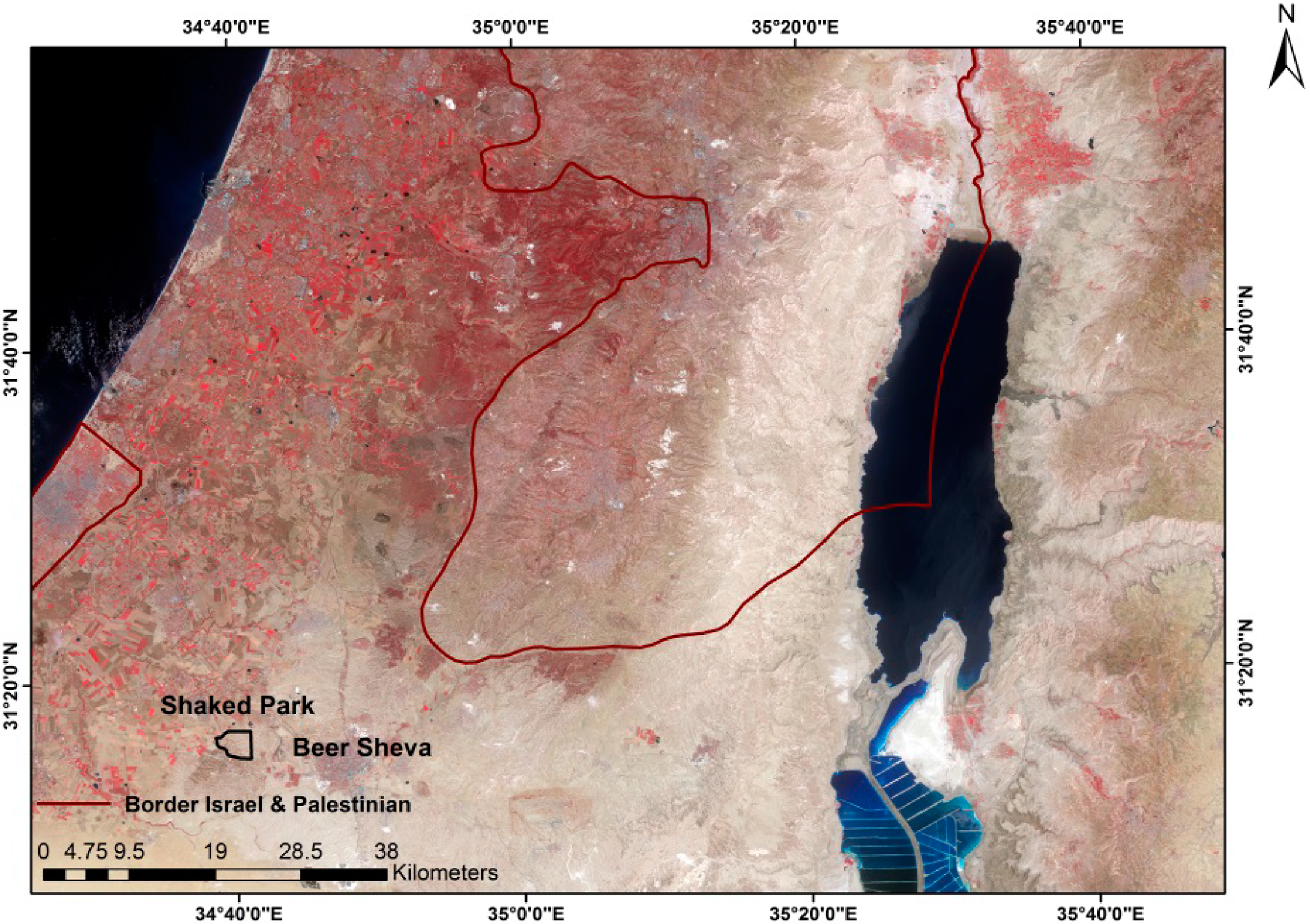
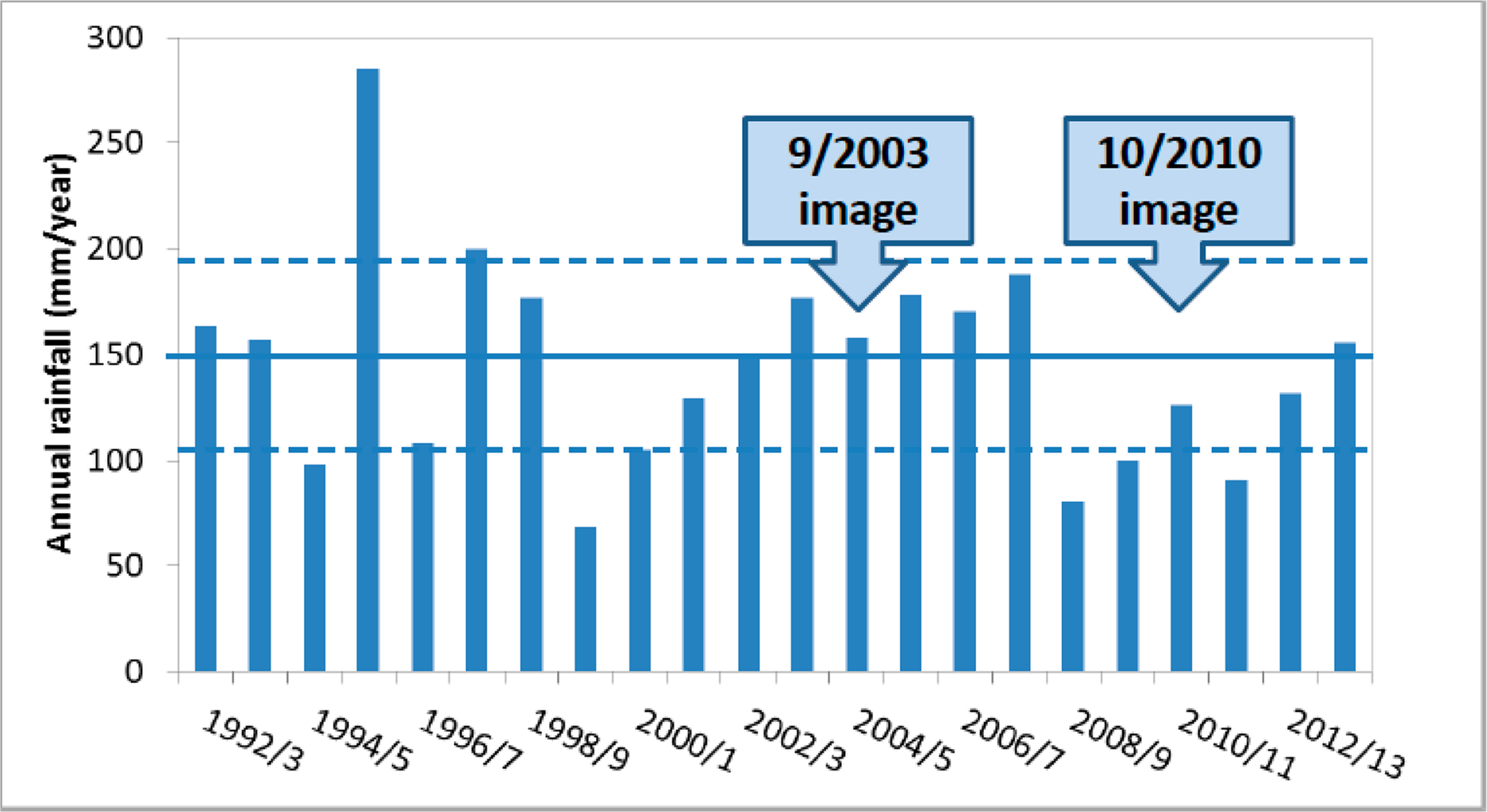
The study site is located within the Shaked Park near Beer-Sheva in the northern Negev Desert of Israel (31°17′N, 34°37′E, 190–200 m a.m.s.l.), which is a long-term ecological research (LTER) site (Figure 1). Climatically, the park lies in a transition zone between an arid climate zone and the Mediterranean climate (Figure 1). Average annual rainfall is approximately 150 mm (±48.8 mm standard deviation) (Figure 2), most of which occurs between November and March. The soil in general is loessial, about 1 m thick, and consists of 14% clay, 27% silt and 59% sand (USA classification: loess soil with sandy loam texture) on an Eocene chalky bedrock. The natural landscape is composed of a series of discontinuous shrub mounds within a matrix of biocrusts. The small patches of shrubs include mainly Noaea mucronata, Atractylis serratuloides and Thymelaea hirsuta. The biocrusts, which cover about 75% of the soil surface, consist of cyanobacteria, bacteria, algae and lichens [4,44]. The surface of the soil crust is flat and solid, because of the soil particle adhesion caused by polysaccharides, excreted mainly by cyanobacteria and soil algae [45]. The total area of the study system is 445 ha and includes different management regimes: (1) desertified shrubland with no grazing in the LTER (30 ha); (2) desertified shrubland with grazing; (3) managed RHS of 150 ha that was developed in 1985–1987 and consists of contour catchments on hill-slope and mini-catchments as management practices to create sink patches; (4) unmanaged RHS; and (5) a managed river stream area. In the Shaked Park, a series of drought events occurred in September 2008, and October 2009, with 80.0 and 100.0 mm of rain, respectively (Figure 2). Note that the rainfall amounts in these years were below 1 standard deviation from the long-term annual mean. These consecutive two drought years caused large shrub mortality, along with severe reduction in the vegetation cover on the hill slopes and along the river streams. This unique phenomenon was the driver for the current research.

2.2. Vegetation Cover

The vegetation cover provides a comprehensive evaluation of the ecosystem state and services, including measures of changes in ecosystem function [46–50]. In the present study, the woody vegetation cover at the end of the dry season (in the years 2003 and 2010) was evaluated, by calculating the commonly used NDVI, using remote sensing data [42,51]:

$$\text{NDVI}=\frac{\left({\rho }_{\mathit{NIR}}-{\rho }_R\right)}{\left({\rho }_{\mathit{NIR}}+{\rho }_R\right)}$$

(1)

where ρ_x is the reflectance at the given wavelength (Equation (1)). The NDVI is based on the contrast between the maximum radiation absorption of red (R, 600–700 nm), due to chlorophyll pigments, and the maximum reflectance in the near infrared (NIR, 700–1200 nm), caused by leaf cellular structure and the fact that soil spectra, lacking these mechanisms, typically do not show such a dramatic spectral difference. The satellite sensor data-based NDVI is often used as an indicator of vegetation activity, as it exhibits a nearly linear relationship with the fraction of photosynthetically-active radiation absorbed by the vegetation canopy [52] and also with net primary production (NPP) [53]. In addition, the NDVI is a powerful monitoring tool for identifying changes of vegetation state in response to drought and climatic change [54]. Using spectral wavebands, this index is quantified by the abovementioned equation (Equation (1)). The NDVI values range between −1 and +1. A value of zero means no vegetation, while values close to +1 (0.8–0.9) indicate the highest vegetation index (green leaves).

2.3. Biocrust Cover

Several indices were used to identify and map cyanobacteria-dominated biocrusts [43] and lichen-dominated biocrusts using multispectral remote sensing [55] and hyperspectral imaging [56]. Other studies use different band combinations in different spectral regions for assessing the development of biocrusts [57,58]. In the current study, the evaluation of the biocrusts was calculated by the CI, using remote sensing data. This index aims to differentiate between crusted and uncrusted areas and to identify areas with different fine and organic matter contents [43]:

$$\text{CI}=1-\frac{\left({\rho }_R-{\rho }_B\right)}{\left({\rho }_R+{\rho }_B\right)}$$

(2)

where ρ_R and ρ_B are the reflectance in the red (R, 600–700 nm) and in the blue (B, 400–500 nm) spectral bands, respectively (Equation (2)). The CI takes advantage of a unique spectral feature of soil biocrusts containing cyanobacteria. It has been shown that the special phycobilin pigment in cyanobacteria contributes in producing a relatively higher reflectance in the blue spectral region than the same type of substrate without a biocrust. As a mapping tool, the CI image was found to be much more sensitive to the ground features than the original images. The absence, existence and distribution of soil crust are important information for desertification and climate change studies. CI values range between 0 and +2, but are typically between 0 and +1 [43,59]. The addition of 1 to the result is for obtaining the normalized difference and is recommended in order to create higher values for soils with high fine and organic matter contents. To avoid vegetation effects (photosynthetically-active radiation), all of the woody vegetation had been masked, based on the landscape cover classification, before processing the CI image.

2.4. Landscape Cover Classification

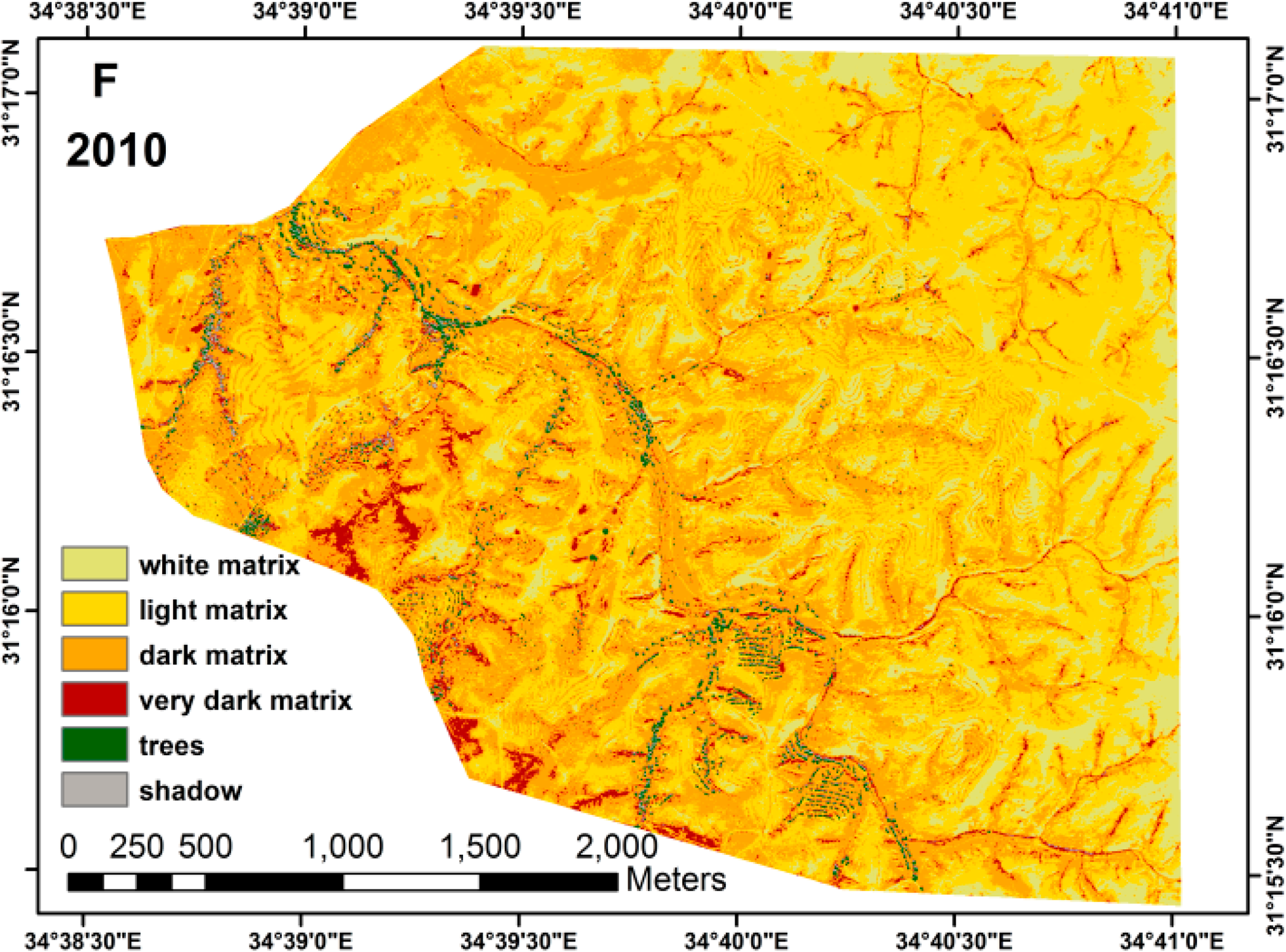
The landscape cover classification was carried out using a support vector machine (SVM) classification [60]. ENVI software was used for creating six classes, namely: trees and woody vegetation, white matrix (representing roads, bare soil and exposed rocks), light matrix (mainly representing light biocrusts), dark matrix (mainly representing pit and sink areas with soil organic matter and plant litter), very dark matrix (mainly representing high soil organic matter, plant litter and depressions) and shadow. The classification model was developed from 1500 calibration points in each class. This technique was followed by an accuracy assessment procedure using a high resolution orthophoto (2-m spatial resolution) with 500 validation points in each class. In addition, field measurements were performed to validate the accuracy assessment. The classification accuracy assessment and evaluation were quantified by the kappa coefficient, and the overall accuracy that was calculated from an error (confusion) matrix [61,62].

2.5. Data Analysis: Input to the Model

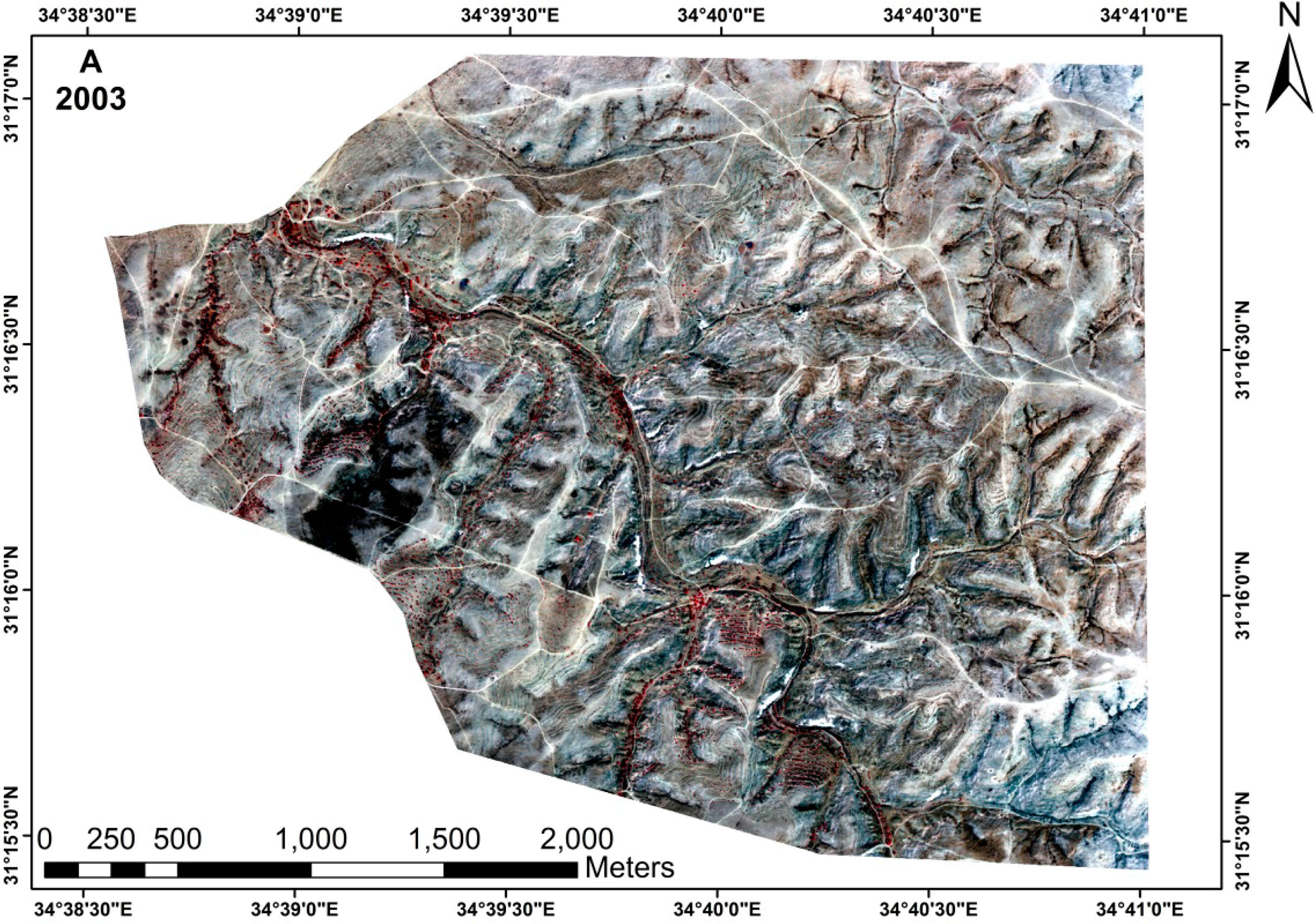
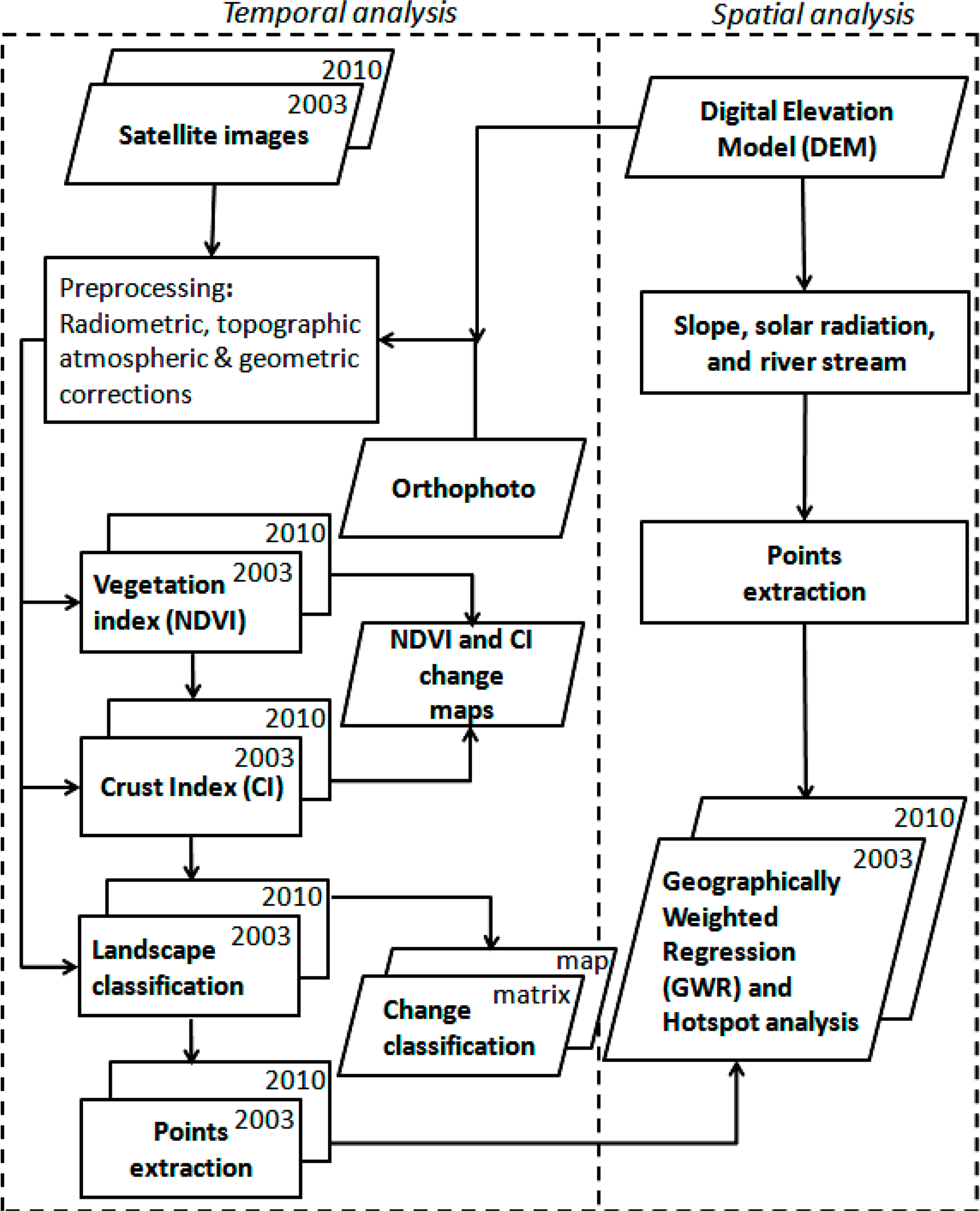
The study evaluated the effect of temporal and spatial changes in the desertified shrublands and in the RHS. The purpose of the temporal analysis process was to gain a better understanding regarding the effect of drought events on vegetation, biocrust and landscape cover changes in these systems. Three main indices were calculated: NDVI for vegetation cover, CI for biocrust cover and landscape cover for landscape classification. The purpose of the spatial analysis process was to gain a better understanding regarding the environmental factors that spatially affect the NDVI and CI after drought events. The temporal analyses included several inputs and preprocessing methods. Two images with a high spatial resolution (2.5 m) and four multispectral bands were selected. The first was a QuickBird image from 17 September 2003, and the second was a WorldView-2 image from 28 October 2010 (Figure 3). The differences between the spectral bands of the two sensors were evaluated, and no significant differences were found. The images were selected from the end of the dry season (after a long dry spell). This enabled the evaluation of the specific effects of the woody vegetation, avoiding the effects of wet soil, annuals and wet biocrusts.

The research flowchart of the preprocessing stages of the temporal and spatial analysis approach is presented in Figure 4. The preprocessing of the images included radiometric, atmospheric, topographic and geometric corrections. The geometric correction was conducted with respect to orthophoto images with a spatial resolution of 2 m. For the topographic correction, a digital elevation model with a spatial resolution of 2 m was used. The root mean square error (RMSE) of the geometric rectification in the 2003 image was 0.98 (with a standard deviation (SD) of 0.46 per pixel), and for the 2010 image, the RMS was 1.75 (with SD 0.75 per pixel). The radiometric correction (including the atmospheric correction) and the topographic correction were performed with ATCOR3 software. We used the NDVI, CI and the landscape classification changes by two change detection models. The spatial analyses (environmental variables) included solar radiation (representing the aspect of the detected area) and slope layers extracted from the digital elevation model (DEM, 2-m resolution). The Archydro tool in ArcGIS was used to create the river stream layer. These inputs were used to identify the spatial and temporal changes in the system, by analyzing the whole study system and polygons with respect to the different management regimes (Figure 3B). All selected polygons were within a similar area of 16 ha. In addition, all selected polygons had the same second river stream order.

2.6. Spatial and Temporal Analyses

2.6.1. Change Detection Model

Change detection is the process of identifying differences in the state of an object or phenomenon by observing it in different periods. It involves the ability to quantify temporal effects using multitemporal datasets. The most commonly used is pixel-by-pixel comparison based on the original spectral information. In this case, the accuracy of the radiometric information between the images, the sensors inputs and the weather conditions between the dates are needed to avoid irrelevant changes [63]. Change detection has become one of the major applications of remote sensing data, because of the repetitive coverage in different time intervals and consistent image quality [64]. There are several methods for detecting land cover changes [65–67]. In the present study, two change detection approaches were used for assessing the main changes in the NDVI, CI and landscape cover, between 2003 and 2010. The first approach was to evaluate the changes within a given land cover type (NDVI and CI). The second approach was to convert between several land cover types (classes) by using a change matrix classification. The first approach was used to evaluate changes in NDVI and CI images (ΔCD) [65]:

$$\Delta \mathit{CD}={\mathit{IMAGE}}_1-{\mathit{IMAGE}}_2$$

(3)

where the subscripts, 1 and 2, represent Dates 1 and 2, respectively, in either the NDVI or the CI images. The results of this operation correspond to an increase or decrease in vegetation or soil cover. A common way to assess changes is based on determining thresholds in terms of standard deviation levels from the mean of ΔCD [68,69]. In this manner, one can distinguish between changed and unchanged pixels, as well as between negative and positive changes [69,70]. In the case of negative changes, the threshold is determined as the maximal value (≈0), and in the case of positive changes, the threshold is determined as the minimal value (≈0), not in adjacency to the mean, in order not to lose meaningful information [66,71]. In the case of the ΔNDVI, changes were analyzed with steps of a half standard deviation, while in the ΔCI case, steps were set to one standard deviation. The selection of the threshold steps in units of standard deviation is based on the dynamic range of the resulting difference data sets.

In order to evaluate the changes in the landscape classification, the second approach of a “change classification matrix” between 2003 and 2010 was used (Figure 4). For each class, the numbers of changed and unchanged pixels were calculated. Furthermore, the total numbers of pixels for each of the six classes were compared between the two images (2003 versus 2010) in order to analyze shifts between classes. Then, the two classification images were overlaid, and a change map was extracted. The output “change classification image” included pixels that were transformed into a different class and unchanged pixels. This was done to evaluate the total change in the classification map. In addition, different changes between classes were converted into a transition matrix and normalized to the total study area. As before, the kappa coefficient and the overall accuracy values were selected for accuracy assessment.

2.6.2. Geostatistics Analysis Models

To evaluate the main environmental effects on NDVI and CI after years of drought, a geostatistics spatial analysis was used. The NDVI and CI prediction values were considered as the dependent variables. Four explanatory variables were examined as predictors in the different years: (1) landscape classification, represented by the landscape cover classification map; (2) aspect [72]; (3) slope; and (4) distances from a river stream. The spatial analysis model requires an input of point features. The images included almost 2 million pixels; therefore, in order to determine the optimal sample size, estimation was applied in which a confidence level of 95% was considered. This resulted in a sample size of about 10,000 points. The 10,000 random points were generated across the different layers, followed by extracting the raster values of each variable layer in associated random points. The two geostatistics analysis models that were used are the geographically weighted regression (GWR) and the hot-spot analysis.

The GWR was designed to consider the location of points, so that spatially varying relationships could be explored [68,73,74]. The model outputs indicate the relations between the NDVI or CI and the four explanatory variables in the different years. The model enables us to understand what effects the explanatory variables have on the variability of NDVI or CI values in the study system. The GWR results include patterns of residuals, residual squares, R² and adjusted and spatial autocorrelation. The model with the highest R² for each explanatory variable or combination of variables has the strongest effect on the NDVI or CI.

The second model, the hot-spot analysis, carried out using the Getis-Ord Gi statistic, was used to define the clustered regions and obtain a z-score output for every point [75]. The z-scores are measures of standard deviation that reflect the significance of the clustering. Extreme z-scores mean maximum clustering. In addition, the hot-spot analysis method indicates whether the cluster has high values (hot spot) or low values (cold spot). The final output displays where high and low values are clustered and whether the clustering is significant.

2.7. Statistical Analysis

Analyses of variances for the change in NDVI and CI between the different polygons were tested using an analysis of variance (ANOVA) for repeated measurement and a one-way ANOVA for the average sample for each polygon. The separation of means was subjected to a Tukey test to detect significant differences. The differences between the change in NDVI and CI values were tested for their level of significance at p = 0.05 between different management regime polygons.

3. Results

3.1. Classification

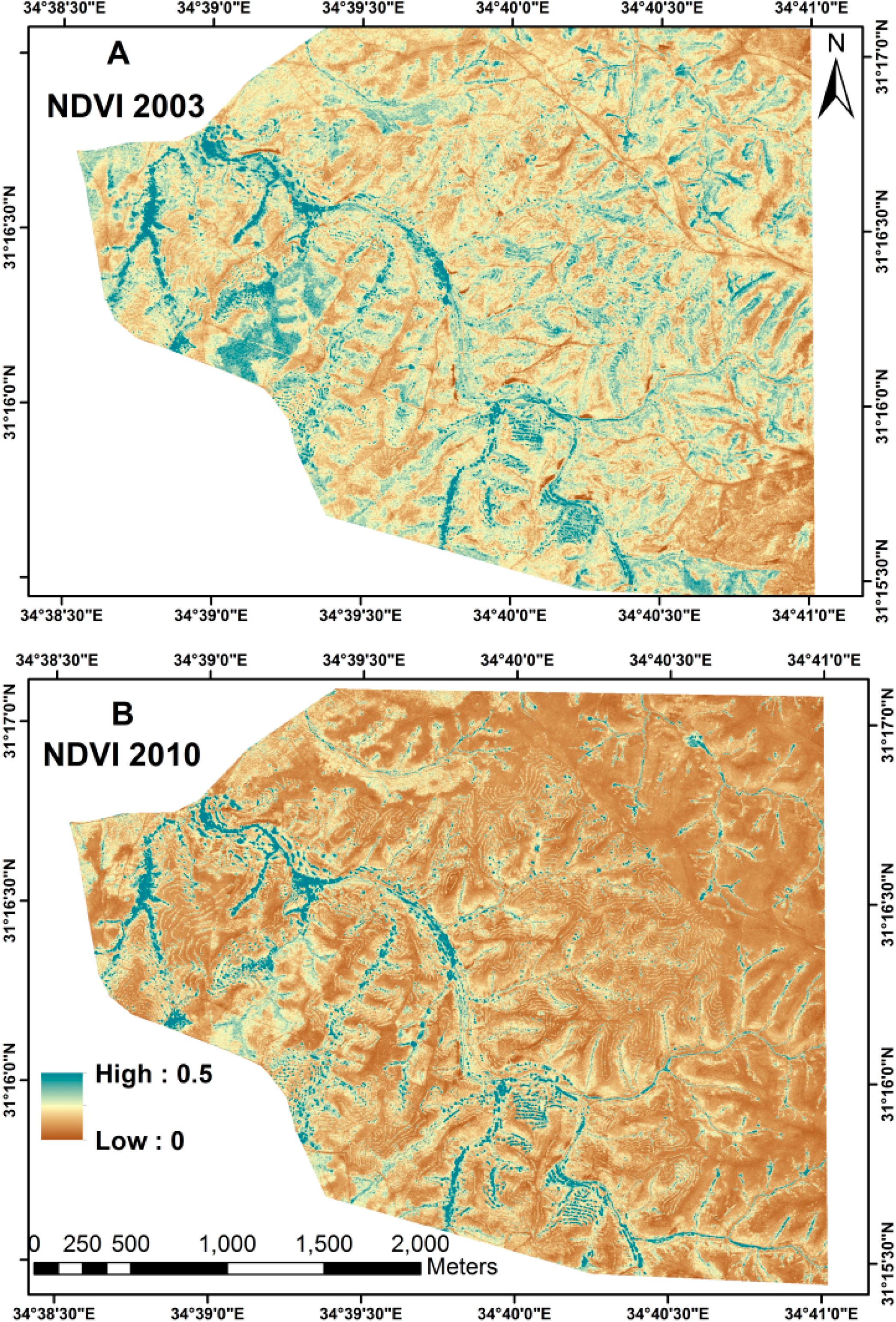
Figure 5A,B presents the vegetation cover, in terms of NDVI, calculated for the years 2003 and 2010. Figure 5C,D presents the biocrust cover, in terms of CI, calculated for the years 2003 and 2010. Figure 5E,F presents the landscape cover classification, classified into six classes, calculated for the years 2003 and 2010. These input results were used to identify the spatial and temporal changes in the system, by analyzing the whole study system and polygons with respect to the different management regimes.

3.2. Identified Changes in Land Cover

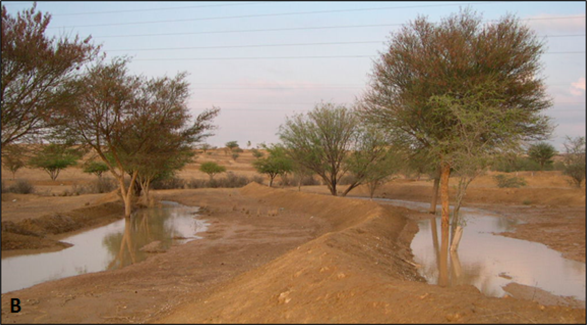
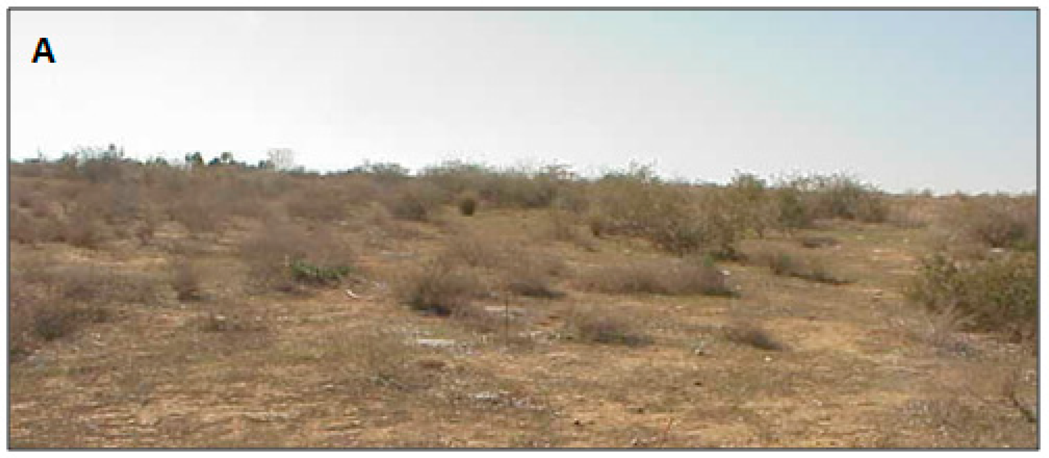
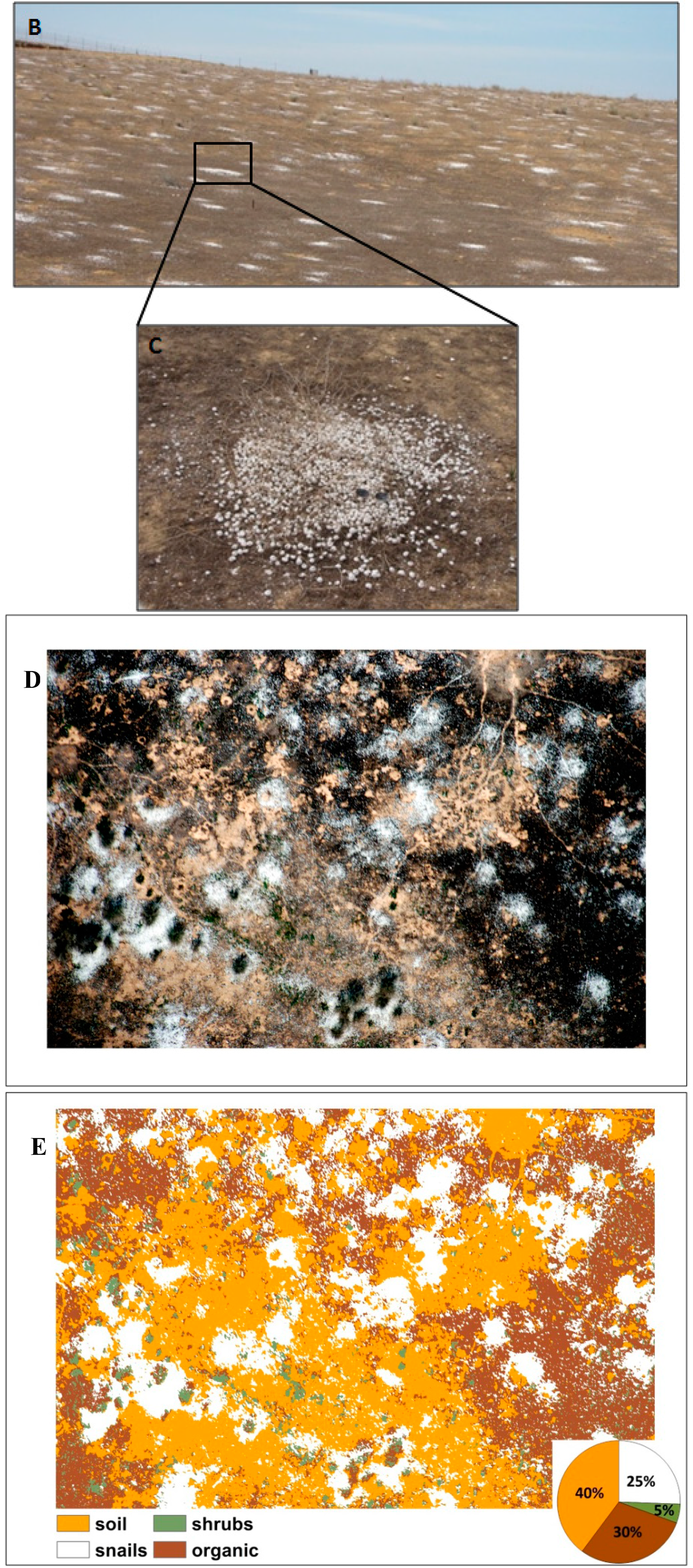
The degradation processes and the mortality of the shrubs in the Shaked Park have been observed as white patches caused by the accumulation of hundreds of shells on the ground. In 2003, before the consecutive drought years, these snails used to feed on and hide in the shrubs (Figure 6A–C). We calculated the land cove features of the desertified shrubland by classifying an airborne image taken in year 2009. The evaluation of the landscape cover included: 39.8% biocrust cover; 29.6% organic matter cover, 25.6% snail shell accumulation; and only 5% woody vegetation cover (shrubs) (Figure 6D–E). This phenomenon of shrub mortality may evidence the degradation processes and the collapse of this shrubland system.

3.3. Change Detection Models

Table 1. . Tables 1.Change detection analysis between images, along with the change statistics, mean and SD, for the NDVI and the CI.

Image 1	Image 2	ΔNDVI		ΔCI
		Mean	SD	Mean	SD
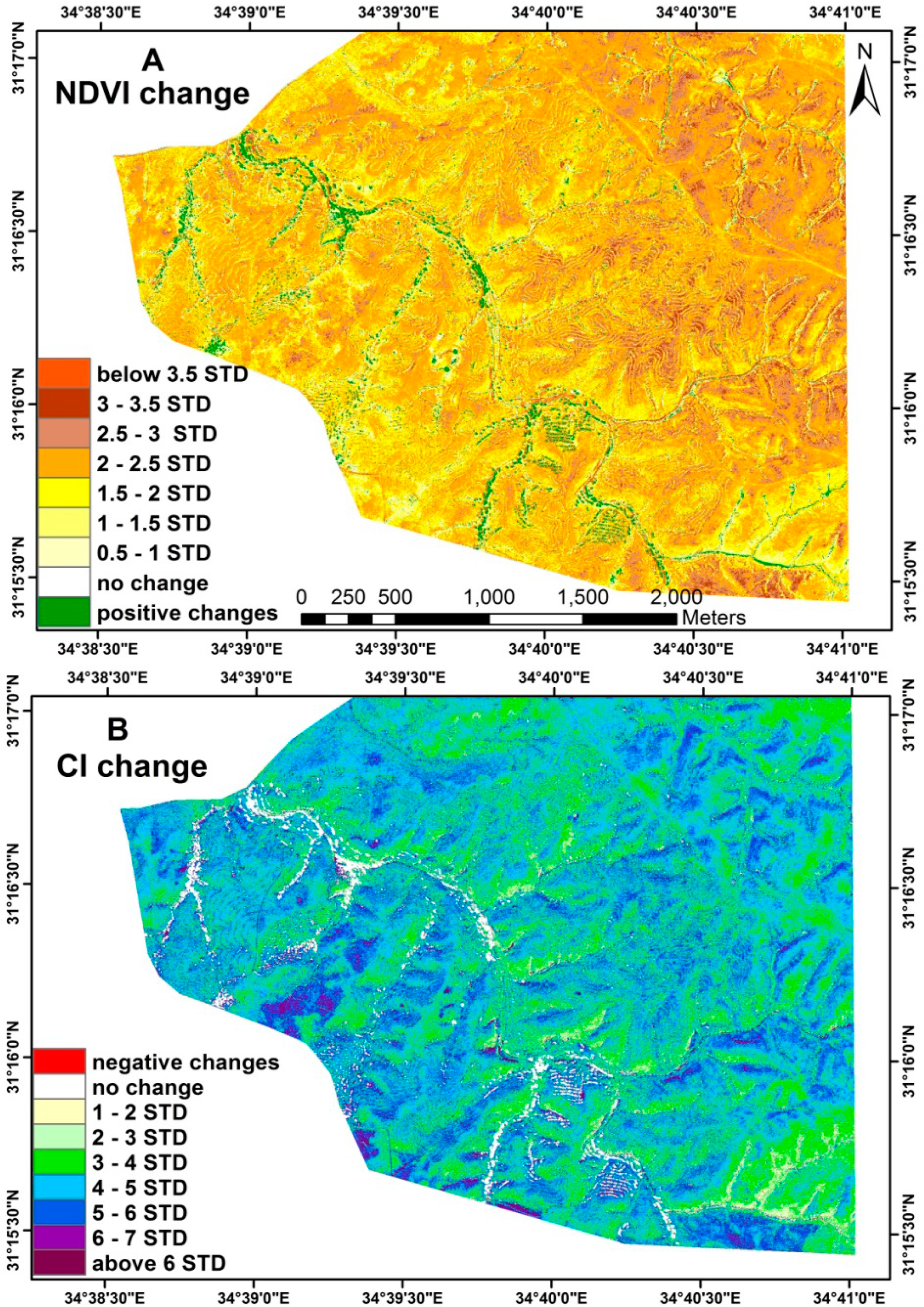
17 September 2003	28 October 2010	−0.83	0.041	0.131	0.03

summarizes the mean and standard deviation (SD) of the two change detection models. Positive means indicate improvement in CI or in NDVI, while negative means indicate degradation. The threshold value was based on SD from the mean change in cases where the mean was between 0.1 and +0.1. When the mean was either smaller than −0.1 or greater than +0.1, the changes were set to zero as the reference point and were not related to the mean. In this study, since NDVI had mainly negative changes, the categories start from zero by adding half an SD towards the negative changes (Figure 7A,C). On the other hand, since CI had mainly positive changes, categories start from zero by adding one SD towards the positive changes (Figure 7B,D).

Table 2. Image differencing results for the NDVI and the CI products for selected images along with the change statistics, mean and SD in different polygons that represent management regimes. The polygons that were significantly different between management regimes are marked in bold.

Polygons for Management Regime	ΔNDVI		ΔCI
	Mean	SD	Mean	SD
Desertified shrubland with no grazing (LTERs)	−0.086 a	0.021	0.149 a	0.031
Desertified shrubland with grazing	−0.098 a	0.025	0.135 a	0.025
Unmanaged RHS	−0.094 a	0.028	0.133 a	0.032
Managed RHS	−0.061 b	0.027	0.137 a	0.034
Managed river stream	−0.061 b	0.025	0.141 a	0.034

Small letters represent significant differences between management regimes.

represents the results of the ΔNDVI and ΔCI for the different polygons. Significant differences were found in the NDVI between the managed RHS and the managed river stream and the other unmanaged regimes, with a considerably higher ΔNDVI. The ΔCI showed positive changes in most of the areas where no significant differences were found between the management regimes.

In addition, change detection products were used in order to analyze category changes in the landscape cover classification. The input to the change classification model included two classification maps. The results of the kappa coefficient and overall accuracy that were calculated from the confusion matrix for the 2003 and 2010 classifications are presented in

Table 3. Kappa coefficient and the overall accuracy for the landscape cover classification input images.

Classification Images	Kappa Coefficient	Overall Accuracy
17 September 2003	93.61%	0.92
28 October 2010	92.26%	0.91

. The change classification matrix is presented in

Table 4. Changes in the landscape cover classification from 2003 to 2010 by class categories. The unchanged pixels are marked in bold along the diagonal.

Classes	Trees and Woody Vegetation	White Matrix	Light Matrix	Dark Matrix	Shadow	Very Dark Matrix
Trees and woody vegetation	10,445	119	459	6741	3497	1836
White matrix	247	140,605	79,989	10,239	67	587
Light matrix	1701	138,631	590,013	221,439	672	6380
Dark matrix	13,835	25,539	259,654	587,707	8155	57,152
Shadow	2741	98	188	3461	2684	1760
Very dark matrix	1342	720	1967	27,961	1773	17,667
Unchanged pixels						1,349,121
Changed pixels						878,950

, showing the shifts between classes. Pixels that have changed from one class to another are presented in Figure 8. This map emphasizes the areas that are undergoing changes in landscape cover. Extensive changes are apparent, mainly in the pit patches of the RHSs that appear as contour lines. Thirty-nine percent of the total study area changed in classification from 2003 to 2010. Among all of the classes, the dark and light matrix classes went through the largest change (16%) of the combined areas of both classes.

Table 5. Number of pixels in each class in the years 2003 and 2010 and the total change in the number of pixels.

Class	Number of Pixels in 2003	Number of Pixels in 2010	Change in the Number of Pixels from 2003 to 2010
Trees and woody vegetation	23,097	30,311	7214
White matrix	231,734	305,712	73,978
Light matrix	958,836	932,270	−26,566
Dark matrix	952,042	857,548	−94,494
Shadow	10,932	16,848	5916
Very dark matrix	51,430	85,382	33,952

presents the changes in the categories of the landscape cover classification from 2003 to 2010. The results show large changes in the number of pixels of the white and dark matrices: an increase in the white matrix, representing an expansion in light biocrusts and bare soil, and a reduction in the dark matrix, representing a decrease in the pit and sink areas and in soil organic matter.

3.4. GWR Statistical Tests

The effect of environmental variables (landscape classification, slope, solar radiation and distance from river stream) on NDVI and CI was studied for each of the two years (2003 and 2010). The spatial analysis results for the GWR statistical tests are shown in

Table 6. GWR results for the NDVI extracted from the images in the years 2003 and 2010, as the dependent variable, versus the explanatory environmental variables. The bold values are the highest R² results for each year.

Dependent Field and Explanatory Field	R2 (2003)	R2Adjusted (2003)	R2 (2010)	R2Adjusted (2010)
NDVI versus landscape classification	0.58	0.52	0.65	0.60
NDVI versus distance from river stream	0.47	0.37	0.69	0.62
NDVI versus slope	0.48	0.35	0.68	0.59
NDVI versus solar radiation	0.44	0.33	0.62	0.52
NDVI versus landscape classification and slope	0.706	0.60	0.76	0.68
NDVI versus landscape classification and solar radiation	0.73	0.64	0.77	0.76
NDVI versus solar radiation and slope	0.49	0.33	0.88	0.82
NDVI versus landscape classification, distance from river stream and solar radiation	0.711	0.604	0.83	0.76
NDVI versus distance from river stream and solar radiation	0.52	0.43	0.95	0.93
NDVI versus landscape classification, solar radiation, slope and distance from river stream	0.82	0.74	0.77	0.71

for the NDVI in both years, with the statistical models that were performed, R² and adjusted R² values. The results indicate that in the year 2003, the landscape classification is the best explanatory variable for the NDVI (R² = 0.58 and R²_adjusted = 0.52). Nevertheless, the group of all explanatory variables that gave the best explanation of NDVI in the year 2003 was the combination of all four environmental variables (R² = 0.82 and R²_adjusted = 0.74). However, the GWR results indicate that in the year 2010, the best explanatory variable for the NDVI was distance from river stream (R² = 0.69 and R²_adjusted = 0.62). In both the 2003 and the 2010 results, joined explanatory environmental variables gave higher correlation results for the NDVI. The combination of the variables of distance from river stream, solar radiation and slope showed a higher spatial correlation to the NDVI (R² = 0.95 and R²_adjusted = 0.93). The changes between the years in the environmental explanatory variables of the NDVI can be explained due to the extreme landscape changes in this system.

The results of the GWR statistical tests for the CI in both years are shown in

Table 7. GWR results for the CI extracted from the images in the years 2003 and 2010, as the dependent variable, versus the explanatory environmental variables. The bold values are the highest R² results for each year.

Dependent Field and Explanatory Field	R2 (2003)	R2Adjusted (2003)	R2 (2010)	R2Adjusted (2010)
CI versus landscape classification	0.46	0.39	0.38	0.27
CI versus distance from river stream	0.47	0.37	0.28	0.17
CI versus slope	0.34	0.28	0.25	0.144
CI versus solar radiation	0.63	0.55	0.47	0.36
CI versus landscape classification and slope	0.61	0.46	0.52	0.35
CI versus landscape classification and solar radiation	0.70	0.60	0.62	0.47
CI versus solar radiation and slop	0.59	0.46	0.49	0.30
CI versus landscape classification, distance from river stream and solar radiation	0.75	0.64	0.76	0.69
CI versus distance from river stream, solar radiation and slope	0.78	0.71	0.77	0.71
CI versus landscape classification, distance from river stream, solar radiation and slope	0.79	0.70	0.81	0.72

, with the statistical models that were performed, R² and adjusted R² values. The results showed a similar pattern in both years. They indicate that the solar radiation was the best explanatory variable for the CI in both years (R² = 0.63 and R²_adjusted = 0.55 in 2003, and R² = 0.47 and R²_adjusted = 0.36 in 2010). Furthermore, as in the NDVI results, joined explanatory environmental variables gave higher spatial correlation results for the CI. The best combination of the explanatory environmental variables was the combination of all four environmental variables, showing a higher spatial correlation to the CI than any sole variable in both years (R² = 0.79 and R²_adjusted = 0.70 in 2003, and R² = 0.81 and R²_adjusted = 0.72 in 2010).

3.5. Hotspot Analysis: Spatial Clustering

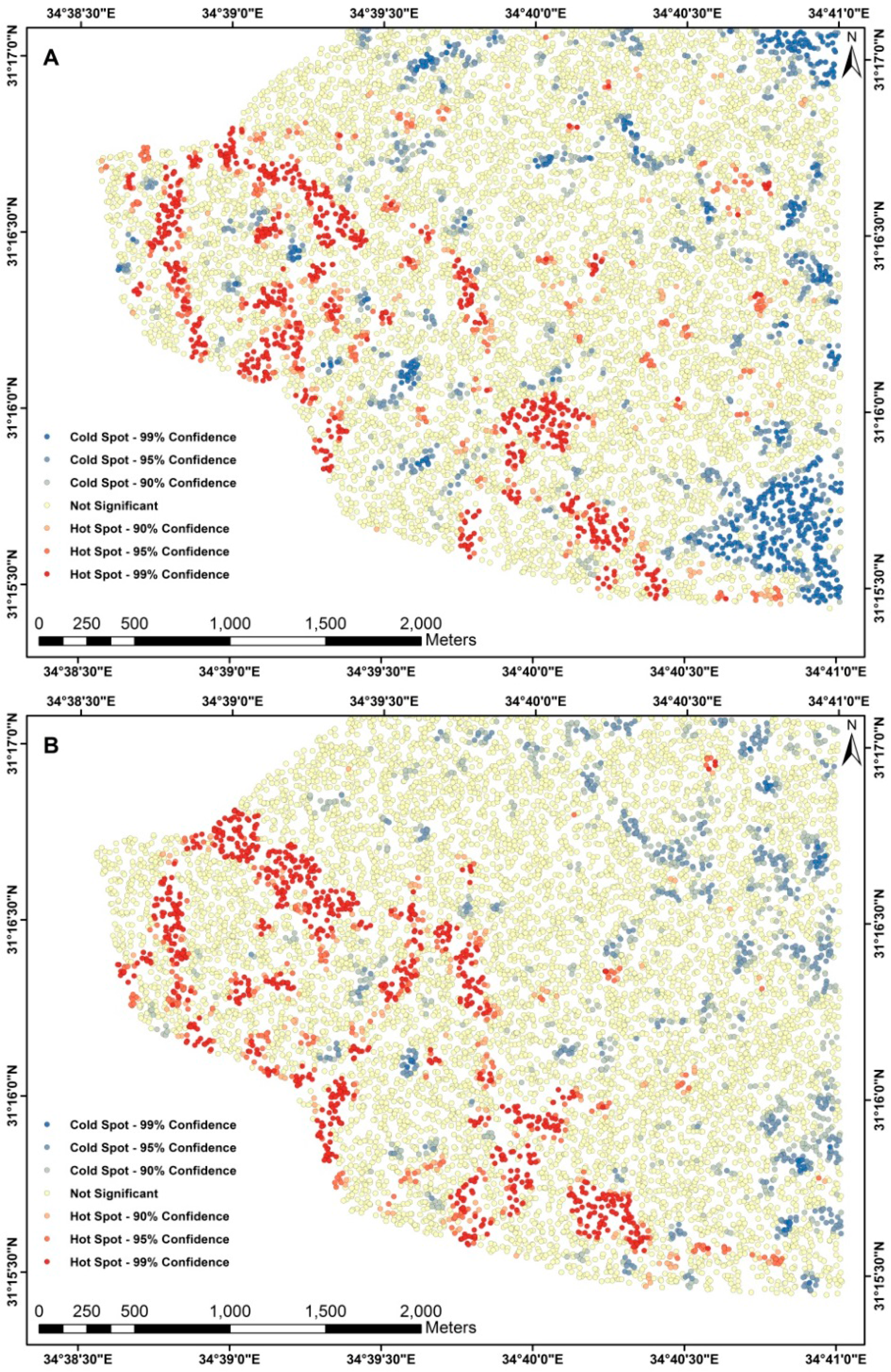
The results of the hotspot analyses for the NDVI with high and low clustering values in 2003 and in 2010 are shown in Figure 9A,B, respectively.

The pattern analysis enables us to observe changes in the spatial cover, created by random processes. Changes in NDVI with significantly high p-values indicate clear clustering, while low p-values mean that the observed spatial pattern is the result of a random process. Statistically, the higher the positive z-score values, the more intense the clustering of high values (hot spot), whereas the more negative the z-score values, the more intense the clustering of low values (cold spot). The results of the hotspot analysis from 2003 show a clear clustering of high values (hot spot) in the large river stream (third stream order) with a high positive z-score. This clustering is intensified in the results from the 2010 hotspot analysis. The results are in accordance with the positive changes in the NDVI, mainly in the large river stream. However, the negative z-scores mainly represent areas with biocrust expansion. In this case, the clustering of cold spots decreased in 2010. These results are also complementary with the CI change model that showed a positive development in the CI, but with no significant differences between the polygons in the different management regimes.

4. Discussion

A drier climate affects ecosystem functions through changes in the landscape structure that, in turn, affect the functional source-sink relations of abiotic and biotic flows through a reduction of the sink patches and an expansion of the source patches [76]. The changes in landscape mosaic determine the spatial distribution of water, transported solutes, sediments, diversity and productivity in dryland systems [5,38,77,78]. In these systems, the eco-hydrological functioning of watersheds on a small scale (within slope flows) and a larger scale (slope-river stream flows) is based on the spatial configuration of runoff-producing source areas (biocrusts) and runoff-absorbing sink areas (shrubs or human-made pits) in the watershed.

Redistribution of water and overland runoff collection by human-made sinks, such as contour catchments, in order to improve productivity, diversity and ecosystem services, are widely used throughout the world (e.g., [33,79–81]). Previous studies have shown that RHSs enhance ecosystem function by increasing soil organic matter accumulation in the pits [4,25,77], increasing active carbon rates and nutrient accumulation, reducing the leakage of resources by accumulating runoff water and nutrients and preventing soil erosion [4,25]. In the current study, we used the knowledge gained about the relationships between the structure and function of natural and human-made, two-phase mosaics on a small scale to interpret them with regard to large-scale changes. We evaluated changes in vegetation, soil and landscape cover on the watershed scale, due to drought events and the effect of human-made RHSs on landscape structure.

4.1. Spatial and Temporal Changes in Vegetation Cover

The negative change in the NDVI shows that the whole system is in a degradation process in relation to energy flow. Drought years seriously affect the amount of water available for the woody vegetation, significantly reducing vegetation production as a result of water shortage. This effect is well demonstrated by the significant decrease in NDVI values in the unmanaged areas between the years 2003 and 2010. However, our results show significantly higher NDVI in the RHS and in the managed river stream. The effect of the RHS redoes the rate of resource leakage on various scales and on energy flow and nutrient fluxes in the ecosystem. However, the reduction in NDVI change values occurs also in the managed RHS and indicates that the whole ecosystem (managed and unmanaged) is under degradation processes. These results can explain the different dynamics of the redistribution of water and nutrients in managed and unmanaged systems on various scales. The significantly higher NDVI values in the managed RHS are due to a reduction in resource leakage through reduced overland runoff-producing, an increase in rainfall absorption and the prevention of soil erosion in the human-made sink patches. The RHS reduces the degradation rate in the system by adding artificial sink patches that overcome the reduction of the natural shrub sink patches as a consequence of drought [4,25,36]. The significantly high NDVI values in the third order river stream can indicate the higher contribution of water, soil, nutrients and organic matter from the crusted slope to the river that has a positive effect on the natural and planted woody vegetation in the river stream. We are, therefore, suggesting that the drought changes the scale of the source-sink relationships; at present, the whole slope, due to a high biocrust cover, is a source of abiotic and biotic flows, and the river is the sink. However, more studies from multiple sites over long-term periods are needed. In addition, additional observation and experimental studies that focus on links and feedbacks between hydrological, pedological and ecological processes at the watershed scale are needed.

The changes that were observed in the GWR model between the years 2003 and 2010 in the environmental variables can explain the spatial variance by the high changes (39%) in the source-sink relationship. These changes are mainly due to the redistribution process of water and sediment. The hotspot analyses showed clear clustering in the third stream order that intensified from 2003 to 2010. The hotspot analysis, showing the processes of resources flowing from the slope into the river streams, suggests that redistribution influences the spatial clustering, not only of soil, vegetation and ecosystem properties [38], but also of hydrological and erosion sedimentation [82], in this degraded ecosystem. However, more hydrological studies are needed.

4.2. Spatial and Temporal Changes of Biocrust Cover

The development of biocrusts in arid lands contributes positively to the soil’s build up, stability, fertility and runoff generation. Additionally, they are of high importance regarding the landscape’s two-phase mosaic structure that drives soil and vegetation patterns and the redistribution of overland runoff in arid areas [4,7,11,83]. However, there is a tipping point where the functioning of the biocrusts changes the state of the system from a resource-conserving ecosystem into a resource-leaking ecosystem. This state change occurs when the crust cover is high in relation to the shrub cover, and this state is a typical desertification state. Therefore, the state of soil crusts within the landscape mosaic is important for desertification determination and for studies of climate change effects on desertification [44,59]. The present study shows the ability to detect and to map biocrust development, in semi-arid areas after drought years and the utility of applying spectral CI as an indicator of desertification processes. The results show positive changes in the CI with the expansion of the biocrusts in the ecosystem. The reduction in the woody vegetation patches and the biocrust expansion increased resource leakage in the ecosystem on the small, as we already indicated [7,11,83], and the large scale. Several studies have shown that on a sandy substrate, biocrusts stabilize shifting dunes [84]. However, on a loess substrate, as in our case, biocrusts increase resource and nutrient loss with runoff [28,44,85] and reduce the ability of plants to germinate [86]. The decreased production resulting from crust patch expansion indicates desertification processes in our study area as a result of high frequency drought events [87]. Therefore, we suggest that CI could be an effective indicator for detecting large-scale desertification processes due to climate change and as a tool for studying biocrust dynamics [84].

CI is an effective indicator due to the signals driven by the external morphology of the biocrusts, whose development and species composition are highly affected by climate (radiation, temperature, soil structure and moisture). Changes in signals are driven by changes in the morphology of the soil crust by biocrust development that is determined by low moisture (drought) and high radiation. This explains why solar radiation was the best explanatory variable for the CI in both years. Other studies have shown that the species composition of biocrusts in the interslope is dependent on radiation [88]. Detecting changes in the morphology of the biocrusts by CI is important for understanding how materials, such as dust, water and seeds, move across the soil surface covering vast regions in drylands worldwide [57]. Therefore, CI could serve as a universal index for determining the function of a two-phase landscape mosaic in relation to its hydro-geological and biological components. CI indicates the potential of the system to retain or lose water, soil and nutrients and to utilize these resources to produce biomass and to conserve biodiversity.

4.3. Spatial Patterns of Landscape Cover’s Structure and Function

This study demonstrates the importance of identifying the combined climate and human-driven landscape cover changes in landscape structure as an indicator for changes in its hydro-ecological functions. In semi-arid areas, the function is dependent on two types of structures: (1) structures that enhance the movement of abiotic and biotic elements across the landscape; and (2) structures that intercept the movement of these elements and conserve them in resource-enriched patches. The first structures are either formed naturally by cyanobacteria, lichens and mosses as ecosystem engineers and are known as biocrusts or by humans using mechanical means and are known as physical crusts (e.g., [4,28,44]). The second structures are either formed naturally by plants and animals or intentionally by humans in the form of pits and mounds. The two types of structures are linked in their functionality; the crust contributes biotic and abiotic elements to the pits and the mounds that make them resource-enriched patches. These processes create a landscape mosaic made of resource-enriched and resource-deprived patches. The number, size and configuration of the two patch types control resource conservation and leakage on the patch, slope, river stream and the watershed scales.

Soil and nutrient conservation and leakage in drylands occur in pulses driven by rainfall duration and intensity [89]. The frequency and magnitude of resource conservation or leakage are controlled by pulse intensity and landscape mosaic, and therefore, they are spatial-scale dependent. Studies have shown that on a slope scale, the magnitude of water leakage increases with the spatial scale [7]. On a watershed scale, studies have found that the frequency of runoff generation in the river streams is negatively related to watershed size [40], whereas the magnitude is positively related to watershed size [40,90]. The scale-dependent principles, in relation to resource conservation and leakage, were demonstrated in this study. Before the drought, due to the high abundance of shrubs on the slope and the river stream, most of the resources were conserved on the slope and in the first order watershed. After the drought, with the increase of CI, water, soil and nutrients leaked from the slope and from the first and second stream order and accumulated in the large river stream (third stream order). The drought-induced changes, on the scale of resource transportation, are the main causes of desertification on the small watershed scales and of the increase of plant productivity in the large river stream.

Our study shows that mapped changes in NDVI and CI across the landscape demonstrate that human intervention, by constructing RHSs, can mitigate the effect of drought and function as a hydro-ecological ecosystem. RHS mimics the function of the shrub patches through the construction of large pits that increase the sink function in the landscape. In addition, the sink function increases by changing the spatial configuration of the pits. While the shrubs form a spot pattern, the contour catchment system creates a bended pattern that prevents resource leakage. In the RHS, water and materials flow from the natural matrix dominated by soil crust to the human-made catchment as an integrated system that forms highly resource-enriched patches.

Our results show that the RHS is an effective system for reducing the rate and counteracting the negative effects of drought. However, more studies from multiple sites over greater time periods are needed. In addition, more observations and experimental studies that are focused on links and feedbacks among hydrological, pedological and ecological processes at the watershed scale are required to validate this conclusion. RHSs prevent leakage, because they are located on the slope where the magnitude of runoff pulses is low [11]. RHS is an adaptive system, functioning as a source-sink system that can be controlled by adjusting: (1) the distances between the banded catchments; (2) the number of banded contour catchments along the slopes; and (3) the proportional size of the contour catchment area in the RHS and the natural source matrix area [4,25]. However, there are constraints on the number of contour catchments, since there is a trade-off between the distribution of runoff to the slope and to the large river stream. Too many contour catchments limit the movement of water to the large river stream and reduce its productivity. This demonstrates the complexity of landscape management through adding sink functions as a means for combating desertification and mitigating climate change.

5. Summary and Conclusions

This study evaluated the changes in soil, vegetation, and landscape cover due to a series of drought years in a managed and unmanaged desertified shrubland in the northern Negev, Israel. This was done using two spectral indices (i.e., NDVI, CI) combined with landscape classification. In addition, the study examined the environmental effects on the indices behavior and their statistical clustering after a drought period. Our main conclusions are as follows:

• Two opposite trends indicate ecosystem degradation (39% of total area). The NDVI shows negative change (mean change = −0.83; SD = 0.041 indicating vegetation reduction) while the CI shows positive change (mean change = 0.131; SD = 0.03 indicating expansion of biocrusts). The measured changes represent redistribution processes of water, sediments, and seeds in a watershed scale.

• The study utilizes a novel combination of a spectral, spatial, and temporal analysis approach based on the use of remote sensing and geographic information systems. With this in mind, short-term landscape changes following a period of successive drought years are identified by the integrated framework.

• More specifically, for the first time spectral CI is applied as a change detection indicator in conjunction with NDVI. This indicator is used to quantify landscape degradation processes in a watershed scale, especially in arid environment where high vegetation is scarce.

• Future studies should test the success of this framework in different sites and different degradation states. In addition, spaceborne remote sensing (multispectral and hyperspectral) can assist in upscaling the hydrological, pedological, and ecological processes to a regional scale.

References

- Valentin, C.; d’Herbès, J.M.; Poesen, J. Soil and water components of banded vegetation patterns. Catena 1999, 37, 1–24. [Google Scholar]
- Mendoza-Aguilar, D.; Cortina, J.; Pando-Moreno, M. Biological soil crust influence on germination and rooting of two key species in a Stipa tenacissima steppe. Plant Soil 2014, 375, 267–274. [Google Scholar]
- Aguiar, M.N.R.; Sala, O.E. Patch structure, dynamics and implications for the functioning of arid ecosystems. Trends Ecol. Evol 1999, 14, 273–277. [Google Scholar]
- Eldridge, D.; Zaady, E.; Shachak, M. Microphytic crusts, shrub patches and water harvesting in the Negev Desert: The shikim system. Landsc. Ecol 2002, 17, 587–597. [Google Scholar]
- Li, X.J.; Li, X.R.; Song, W.M.; Gao, Y.P.; Zheng, J.G.; Jia, R.L. Effects of crust and shrub patches on runoff, sedimentation, and related nutrient (C, N) redistribution in the desertified steppe zone of the Tengger Desert, northern China. Geomorphology 2008, 96, 221–232. [Google Scholar]
- Moreno-de las Heras, M.; Saco, P.M.; Willgoose, G.R.; Tongway, D.J. Assessing landscape structure and pattern fragmentation in semiarid ecosystems using patch-size distributions. Ecol. Appl 2011, 21, 2793–2805. [Google Scholar]
- Shachak, M.; Pickett, S.T.A. Chapter 8. Linking ecological understanding and application: patchiness in a dryland system. In The Ecological Basis for Conservation—Heterogeneity, Ecosystems, and Biodiversity; Pickett, S., Ostfeld, R.S., Shachak, M., Likens, G., Eds.; Springer-Verlag: New York, NY, USA, 1997; Volume 21, pp. 108–119. [Google Scholar]
- Jones, C.G.; Lawton, J.H.; Shachak, M. Positive and negative effects of orfanisms as physical ecosystem engineers. Ecology 1997, 78, 1946–1957. [Google Scholar]
- Segoli, M.; Ungar, D.U.; Shachak, M. Shrube enhance resilience of semi-arid ecosystem by engineering regrowth. Ecohydrology 2008, 1, 330–339. [Google Scholar]
- Segoli, M.; Ungar, E.D.; Shachak, M. Fine-scale spatial heterogeneity of resource modulation in semi-arid “islands of fertility”. Arid Land Res. Manag 2012, 26, 344–354. [Google Scholar]
- Shachak, M.; Sachs, M.; Moshe, I. Ecosystem management of desertified shrublands in Israel. Ecosystems 1998, 1, 475–483. [Google Scholar]
- Easterling, D.R.; Meehl, G.A.; Parmesan, C.; Changnon, S.A.; Karl, T.R.; Mearns, L.O. Climate extremes: Observations, modeling, and impacts. Science 2000, 289, 2068–2074. [Google Scholar]
- De Ridder, K.; Gallée, H. Land surface-induced regional climate change in southern Israel. J. Appl. Meteorol 1998, 37, 1470–1485. [Google Scholar]
- Glantz, M.H.; Orlovsky, N. Desertification: A review of the concept. Desertif. Control Bull 1983, 9, 15–22. [Google Scholar]
- Kefi, S.; Rietkerk, M.; Alados, C.L.; Pueyo, Y.; Papanastasis, V.P.; ElAich, A.; de Ruiter, P.C. Spatial vegetation patterns and imminent desertification in mediterranean arid ecosystems. Nature 2007, 449, 213–217. [Google Scholar]
- Reynolds, J.F.; Smith, D.M.S.; Lambin, E.F.; Turner, B.L.; Mortimore, M.; Batterbury, S.P.J.; Downing, T.E.; Dowlatabadi, H.; Fernández, R.J.; Herrick, J.E.; et al. Global desertification: Building a science for dryland development. Science 2007, 316, 847–851. [Google Scholar]
- Verstraete, M.M.; Schwartz, S.A. Desertification and global change. Vegetation 1991, 91, 3–13. [Google Scholar]
- Ravi, S.; Breshears, D.D.; Huxman, T.E.; D’Odorico, P. Land degradation in drylands: Interactions among hydrologic-aeolian erosion and vegetation dynamics. Geomorphology 2010, 116, 236–245. [Google Scholar]
- Adams, H.D.; Guardiola-Claramonte, M.; Barron-Gafford, G.A.; Villegas, J.C.; Breshears, D.D.; Zou, C.B.; Troch, P.A.; Huxman, T.E. Temperature sensitivity of drought-induced tree mortality portends increased regional die-off under global-change-type drought. Proc. Natl. Acad. Sci. USA 2009, 106, 7063–7066. [Google Scholar]
- Allen, C.D.; Macalady, A.K.; Chenchouni, H.; Bachelet, D.; McDowell, N.; Vennetier, M.; Kitzberger, T.; Rigling, A.; Breshears, D.D.; Hogg, E.H.; et al. A global overview of drought and heat-induced tree mortality reveals emerging climate change risks for forests. For. Ecol. Manag 2010, 259, 660–684. [Google Scholar]
- Dai, A. Drought under global warming: A review. Wiley Interdiscip. Rev.: Clim. Chang 2011, 2, 45–65. [Google Scholar]
- Le Houérou, H.N. Climate change drought and desertification. Arid Environ 1996, 34, 133–185. [Google Scholar]
- Mulligan, M. Modelling the geomorphological impact of climatic variability and extreme events in a semi-arid environment. Geomorphology 1998, 24, 59–78. [Google Scholar]
- Boeken, B.; Orenstein, D. The effect of plant litter on ecosystem properties in a Mediterranean semi-arid shrubland. J. Veg. Sci 2001, 12, 825–832. [Google Scholar]
- Eldridge, D.J.; Zaady, E.; Shachak, M. Infiltration through three contrasting biological soil crusts in patterned landscapes in the Negev, Israel. Catena 2000, 40, 323–336. [Google Scholar]
- West, N.E. Structure and function of microphytic soil crusts in wildland ecosystems of arid to semi-arid regions. In Advances in Ecological Research; Begon, M., Fitter, A.H., Macfadyen, A., Eds.; Academic Press Inc: New York, NY, USA, 1990; Volume 20, pp. 179–223. [Google Scholar]
- KrÖPfl, A.I.; Cecchi, G.A.; Villasuso, N.M.; Distel, R.A. Degradation and recovery processes in semi-arid patchy rangelands of northern Patagonia, Argentina. Land Degrad. Dev 2013, 24, 393–399. [Google Scholar]
- Zaady, E.; Offer, Z.Y.; Shachak, M. The content and contributions of deposited aeolian organic matter in a dry land ecosystem of the Negev Desert, Israel. Atmos. Environ 2001, 35, 769–776. [Google Scholar]
- Bertrand, B.; Shachak, M. Desert plant communities in human-made patches-implications for management. Ecol. Appl 1994, 4, 702–716. [Google Scholar]
- Schlesinger, W.H.; Raikes, J.A.; Hartley, A.E.; Cross, A.F. On the spatial pattern of soil nutrients in desert ecosystems. Ecology 1996, 77, 364–374. [Google Scholar]
- Mussery, A.; Leu, S.; Lensky, I.; Budovsky, A. The effect of planting techniques on arid ecosystems in the northern Negev. Arid Land Res. Manag 2013, 27, 90–100. [Google Scholar]
- Turner, M.G.; O’Neill, R.V.; Gardner, R.H.; Milne, B.T. Effects of changing spatial scale on the analysis of landscape pattern. Landsc. Ecol 1989, 3, 153–162. [Google Scholar]
- Zhang, S.; Carmi, G.; Berliner, P. Efficiency of rainwater harvesting of microcatchments and the role of their design. J. Arid Environ 2013, 95, 22–29. [Google Scholar]
- De Winnaar, G.; Jewitt, G.P.W.; Horan, M. A. GIS-based approach for identifying potential runoff harvesting sites in the Thukela River Basin, South Africa. Phys. Chem. Earth Parts A/B/C 2007, 32, 1058–1067. [Google Scholar]
- Sache, M.; Moshe, I. Savannization: An ecologecal vible menagement approach to desertified regions. In Arid Lands Management: Toward Ecological Sustainability; Hoekstra, T., Moshe, S., Eds.; University of Illinois Press: Champaign, IL, USA, 1999; pp. 248–253. [Google Scholar]
- Zaady, E.; Shachak, M.; Moshe, I. Ecological approach for afforestation in arid regions of the northern Negev Desert, Israel. In Deforestation, Environment, and Sustainable Development: A Comparative Analysis; Vajpeyi, D.K., Ed.; Greenwood Publishing Group, Inc.: Praeger, CT, USA, 2001; pp. 219–238. [Google Scholar]
- Buis, E.; Veldkamp, A. Modelling dynamic water redistribution patterns in arid catchments in the Negev Desert of Israel. Earth Surf. Process. Landf 2008, 33, 107–122. [Google Scholar]
- Imeson, A.C.; Prinsen, H.A.M. Vegetation patterns as biological indicators for identifying runoff and sediment source and sink areas for semi-arid landscapes in Spain. Agric. Ecosyst. Environ 2004, 104, 333–342. [Google Scholar]
- Maestre, F.; Cortina, J. Spatial patterns of surface soil properties and vegetation in a Mediterranean semi-arid steppe. Plant Soil 2002, 241, 279–291. [Google Scholar]
- Karnieli, A.; Ben-Asher, J.; Dodi, A.; Issar, A.; Oron, G. An empirical approach for predicting runoff yield under desert conditions. Agric. Water Manag 1988, 14, 243–252. [Google Scholar]
- Mu, Q.; Zhao, M.; Kimball, J.S.; McDowell, N.G.; Running, S.W. A remotely sensed global terrestrial drought severity index. Bull. Am. Meteorol. Soc 2012, 94, 83–98. [Google Scholar]
- Tucker, C.J.; Slayback, D.A.; Pinzon, J.E.; Los, S.O.; Myneni, R.B.; Taylor, M.G. Higher northern latitude normalized difference vegetation index and growing season trends from 1982 to 1999. Int. J. Biometeorol 2001, 45, 184–190. [Google Scholar]
- Karnieli, A. Development and implementation of spectral crust index over dune sands. Int. J. Remote Sens 1997, 18, 1207–1220. [Google Scholar]
- Grishkan, I.; Zaady, E.; Nevo, E. Soil crust microfungi along a southward rainfall gradient in desert ecosystems. Eur. J. Soil Biol 2006, 42, 33–42. [Google Scholar]
- Zaady, E.; Groffman, P.; Shachak, M. Nitrogen fixation in macro- and micro-phytic patches in the Negev Desert. Soil Biol. Biochem 1998, 30, 449–454. [Google Scholar]
- Carter, M.R. Soil quality for sustainable land management: Organic matter and aggregation interactions that maintain soil functions. Agronomy 2002, 94, 38–47. [Google Scholar]
- Running, S.; Loveland, T.R.; Pierce, L.L.; Nemani, R.R.; Hunt, E.R. A remote sensing based vegetation classification logic for global land cover analysis. Remote Sens. Environ 1995, 51, 39–48. [Google Scholar]
- Running, S.W.; Coughl, J.C. A general model of forest ecosystem processes for regional applications I. Hydrological balance, canopy gas exchange and primary production processes. Ecol. Model 1988, 42, 125–154. [Google Scholar]
- Running, S.W.; Nemani, R.; Heinsch, F.; Zhao, M.; Reeves, M.; Hashimoto, H. A continuous satellite-derived measure of global terrestrial primary production. BioScience 2004, 54, 547–560. [Google Scholar]
- TurHorst, C.P.; Munguia, P. Measuring ecosystem function: Consequences arising from variation in biomass-productivity relationships. Community Ecol 2008, 9, 39–44. [Google Scholar]
- Carlson, T.N.; Ripley, D.A. On the relation between NDVI, fractional vegetation cover, and leaf area index. Remote Sens. Environ 1997, 62, 241–252. [Google Scholar]
- Blackburn, G.A. Spectral indices for estimating photosynthetic pigment concentrations: A test using senescent tree leaves. Int. J. Remote Sens 1998, 19, 657–675. [Google Scholar]
- Goward, S.; Tucker, C.; Dye, D. North American vegetation patterns observed with the NOAA-7 Advanced Very High Resolution Radiometer. Vegetatio 1985, 64, 3–14. [Google Scholar]
- Ichii, K.; Kawabata, A.; Yamaguchi, Y. Global correlation analysis for NDVI and climatic variables and NDVI trends: 1982–1990. Int. J. Remote Sens 2002, 23, 3873–3878. [Google Scholar]
- Chen, J.; Zhang, M.Y.; Wang, L.; Shimazaki, H.; Tamura, M. A new index for mapping lichen-dominated biological soil crusts in desert areas. Remote Sens. Environ 2005, 96, 165–175. [Google Scholar]
- Weber, B.; Olehowski, C.; Knerr, T.; Hill, J.; Deutschewitz, K.; Wessels, D.C.J.; Eitel, B.; Büdel, B. A new approach for mapping of biological soil crusts in semidesert areas with hyperspectral imagery. Remote Sens. Environ 2008, 112, 2187–2201. [Google Scholar]
- Rozenstein, O.; Karnieli, A. Identification and characterization of biological soil crusts in a sand dune desert environment across Israel-Egypt border using LWIR emittance spectroscopy. J. Arid Environ 2014. [Google Scholar] [CrossRef]
- Qin, Z.; Li, W.; Burgheimer, J.; Karnieli, A. Quantitative estimation of land cover structure in an arid region across the Israel-Egypt border using remote sensing data. J. Arid Environ 2006, 66, 336–352. [Google Scholar]
- Karnieli, A.; Kidron, G.J.; Glaesser, C.; Ben-Dor, E. Spectral characteristics of cyanobacteria soil crust in semiarid environments. Remote Sens. Environ 1999, 69, 67–75. [Google Scholar]
- Melgani, F.; Bruzzone, L. Classification of hyperspectral remote sensing images with support vector machines. IEEE Trans. Geosci. Remote Sens 2004, 42, 1778–1790. [Google Scholar]
- Congalton, R.G. A review of assessing the accuracy of classifications of remotely sensed data. Remote Sens. Environ 1991, 37, 35–46. [Google Scholar]
- Foody, G.M. Status of land cover classification accuracy assessment. Remote Sens. Environ 2002, 80, 185–201. [Google Scholar]
- Lu, D.; Mausel, P.; Brondízio, E.; Moran, E. Change detection techniques. Int. J. Remote Sens 2004, 25, 2365–2401. [Google Scholar]
- Tian, J.; Cui, S.; Reinartz, P. Building change detection based on satellite stereo imagery and digital surface models. IEEE Trans. Geosci. Remote Sens 2014, 52, 406–417. [Google Scholar]
- Mas, J.F. Monitoring land-cover changes: A comparison of change detection techniques. Int. J. Remote Sens 1999, 20, 139–152. [Google Scholar]
- Lambin, E.F.; Strahlers, A.H. Change-vector analysis in multitemporal space: A tool to detect and categorize land-cover change processes using high temporal-resolution satellite data. Remote Sens. Environ 1994, 48, 231–244. [Google Scholar]
- Johnson, R.D.; Kasischke, E.S. Change vector analysis: A technique for the multispectral monitoring of land cover and condition. Int. J. Remote Sens 1998, 19, 411–426. [Google Scholar]
- Foody, G.M. Geographical weighting as a further refinement to regression modelling: An example focused on the NDVI–rainfall relationship. Remote Sens. Environ 2003, 88, 283–293. [Google Scholar]
- Volcani, A.; Karnieli, A.; Svoray, T. The use of remote sensing and gis for spatio-temporal analysis of the physiological state of a semi-arid forest with respect to drought years. For. Ecol. Manag 2005, 215, 239–250. [Google Scholar]
- Justice, C.O.; Townshend, J.R.G.; Holben, B.N.; Tucker, C.J. Analysis of the phenology of global vegetation using meteorological satellite data. Int. J. Remote Sens 1985, 6, 1271–1318. [Google Scholar]
- Lambin, E.F.; Strahler, A.H. Indicators of land-cover change for change-vector analysis in multitemporal space at coarse spatial scales. Int. J. Remote Sens 1994, 15, 2099–2119. [Google Scholar]
- Kumar, L.; Skidmore, A.K.; Knowles, E. Modelling topographic variation in solar radiation in a GIS environment. Int. J. Geogr. Inf. Sci 1997, 11, 475–497. [Google Scholar]
- Wang, Q.; Ni, J.; Tenhunen, J. Application of a geographically-weighted regression analysis to estimate net primary production of chinese forest ecosystems. Glob. Ecol. Biogeogr 2005, 14, 379–393. [Google Scholar]
- Brunsdon, C.; Fotheringham, S.; Charlton, M. Geographically weighted regression. J. R. Stat. Soc.: Ser. D (Stat.) 1998, 47, 431–443. [Google Scholar]
- Reese, D.C.; Brodeur, R.D. Identifying and characterizing biological hotspots in the northern California current. Deep Sea Res. Part II: Top. Stud. Oceanogr. 2006, 53, 291–314. [Google Scholar]
- Opdam, P.; Wascher, D. Climate change meets habitat fragmentation: Linking landscape and biogeographical scale levels in research and conservation. Biol. Conserv. 2004, 117, 285–297. [Google Scholar]
- Boeken, B.; Shachak, M. Colonization by annual plants of an experimentally altered desert landscape: Source-sink relationships. J. Ecol 1998, 86, 804–814. [Google Scholar]
- Porporato, A.; D’Odorico, P.; Laio, F.; Ridolfi, L.; Rodriguez-Iturbe, I. Ecohydrology of water-controlled ecosystems. Adv. Water Res 2002, 25, 1335–1348. [Google Scholar]
- Mbilinyi, B.P.; Tumbo, S.D.; Mahoo, H.F.; Senkondo, E.M.; Hatibu, N. Indigenous knowledge as decision support tool in rainwater harvesting. Phys. Chem. Earth Parts A/B/C 2005, 30, 792–798. [Google Scholar]
- Critchley, W.; Siegert, K. A Manual for the Design and Construction of Water Harvesting Schemes for Plant Production; Food and Agriculture Organization of the United Nations: Rome, Italy, 1991. [Google Scholar]
- Falkenmark, M.; Fox, P.; Persson, G.; Rockstroem, J. Water harvesting for upgrading of rainfed agriculture. In Problem Analysis and Research Needs; SIWI Report II; Stockholme International Water Institute: Sveavagen, Sweden, 2001; pp. 76–87. [Google Scholar]
- Pickup, G. The erosion cell—A geomorphic approach to landscape classification in range assessment. Rangel J 1985, 7, 114–121. [Google Scholar]
- Shoshany, M.; Lavee, H.; Kutiel, P. Seasonal vegetation cover changes as indicators of soil types along a climatological gradient: A mutual study of environmental patterns and controls using remote sensing. Int. J. Remote Sens 1995, 16, 2137–2151. [Google Scholar]
- Zaady, E.; Katra, I.; Yizhaq, H.; Kinast, S.; Ashkenazy, Y. Inferring the impact of rainfall gradient on biocrusts’ developmental stage and thus on soil physical structures in sand dunes. Aeolian Res 2014, 13, 81–89. [Google Scholar]
- Maestre, F.T.; Huesca, M.; Zaady, E.; Bautista, S.; Cortina, J. Infiltration, penetration resistance and microphytic crust composition in contrasted microsites within a mediterranean semi-arid steppe. Soil Biol. Biochem 2002, 34, 895–898. [Google Scholar]
- Zaady, E.; Gutterman, Y.; Boeken, B. The germination of mucilaginous seeds of t Plantago coronopus, Reboudia pinnata, and t Carrichtera annua on cyanobacterial soil crust from the Negev Desert. Plant Soil 1997, 190, 247–252. [Google Scholar]
- Shachak, M.; Lovett, G.M. Atmospheric deposition to a desert ecosystem and its implications for management. Ecol. Appl 1998, 8, 455–463. [Google Scholar]
- Nevo, E. “Evolution canyon”: A microcosm of life’s evolution focusing on adaptation and speciation”. Isr. J. Ecol. Evol 2006, 52, 501–506. [Google Scholar]
- Noy-Meir, I. Desert ecosystems: Environment and producers. Annu. Rev. Ecol. Syst 1973, 4, 25–51. [Google Scholar]
- Evenari, M.; Shanan, L.; Tadmor, N. The Negev: The Challenge of a Desert; Oxford University Press: London, UK, 1983. [Google Scholar]