
The Ground-Based Absolute Radiometric Calibration of Landsat 8 OLI

 and
and
Abstract
:
1. Introduction

| OLI | ETM+ | ||
|---|---|---|---|
| Band | Center Wavelength (nm) | Band | Center Wavelength (nm) |
| 1 | 443.0 | -- | -- |
| 2 | 482.6 | 1 | 478.7 |
| 3 | 561.3 | 2 | 561.0 |
| 4 | 654.6 | 3 | 661.4 |
| 5 | 864.6 | 4 | 834.6 |
| 6 | 1609.1 | 5 | 1650.3 |
| 7 | 2201.3 | 7 | 2208.2 |
| 8 (Pan) | 591.7 | 8 (Pan) | 720.1 |
2. Methodology
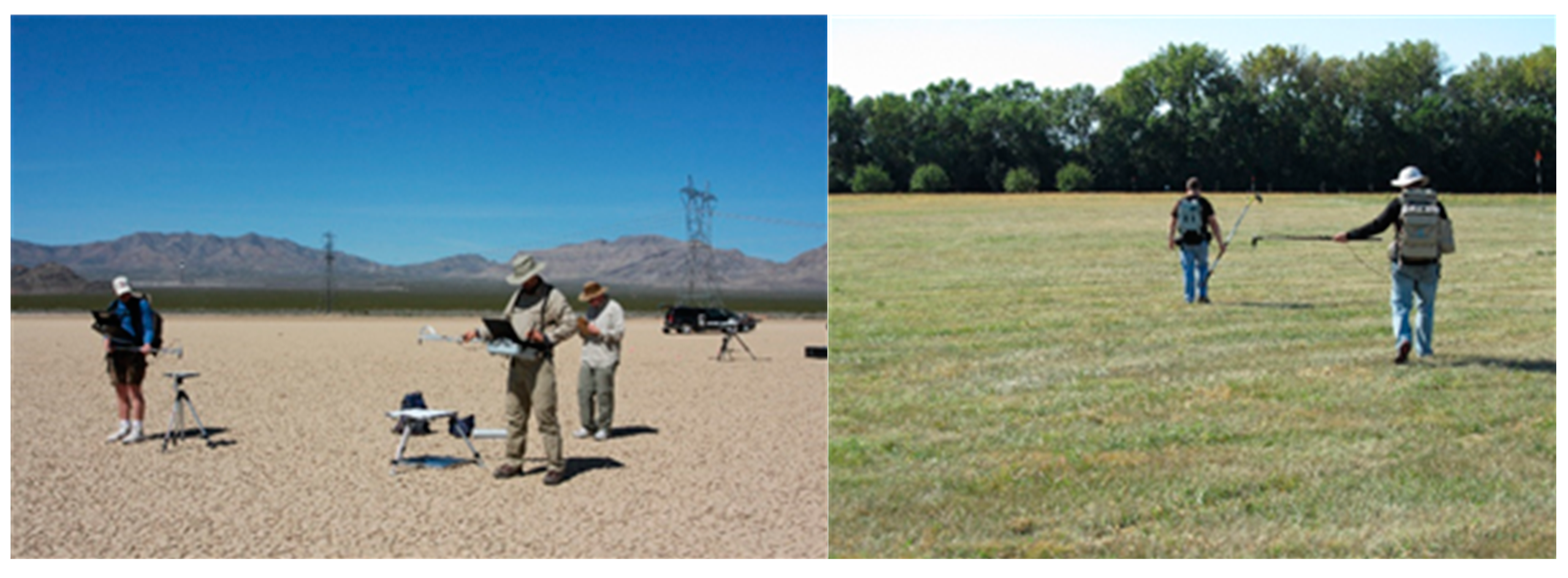
2.1. Reflectance-Based Approach to Vicarious Calibration

2.1.1. Surface Reflectance


2.1.2. Atmospheric Measurements
2.1.3. Top-of-Atmosphere Spectral Radiance and Reflectance
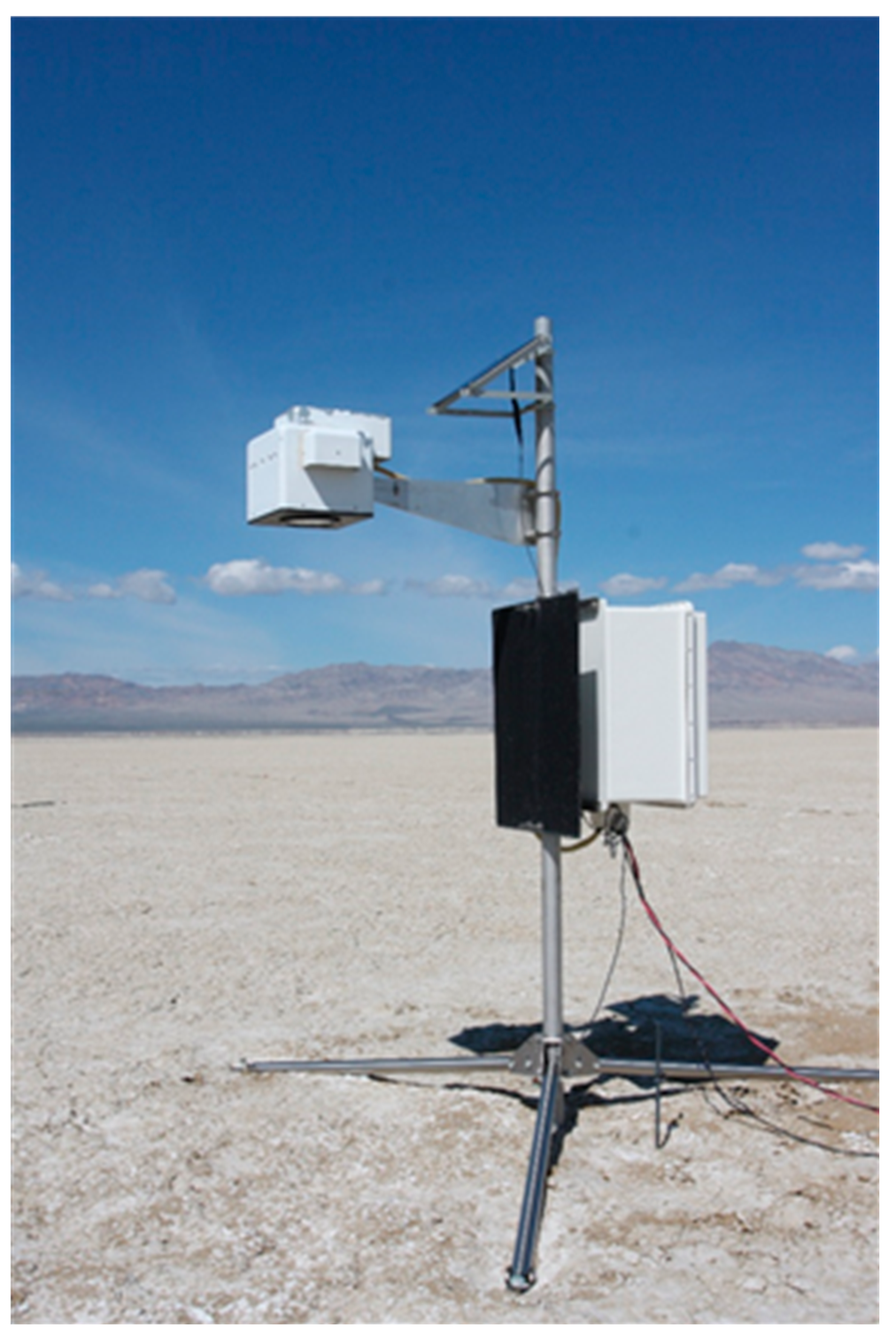
2.2. The Radiometric Calibration Test Site (RadCaTS) at Railroad Valley, Nevada
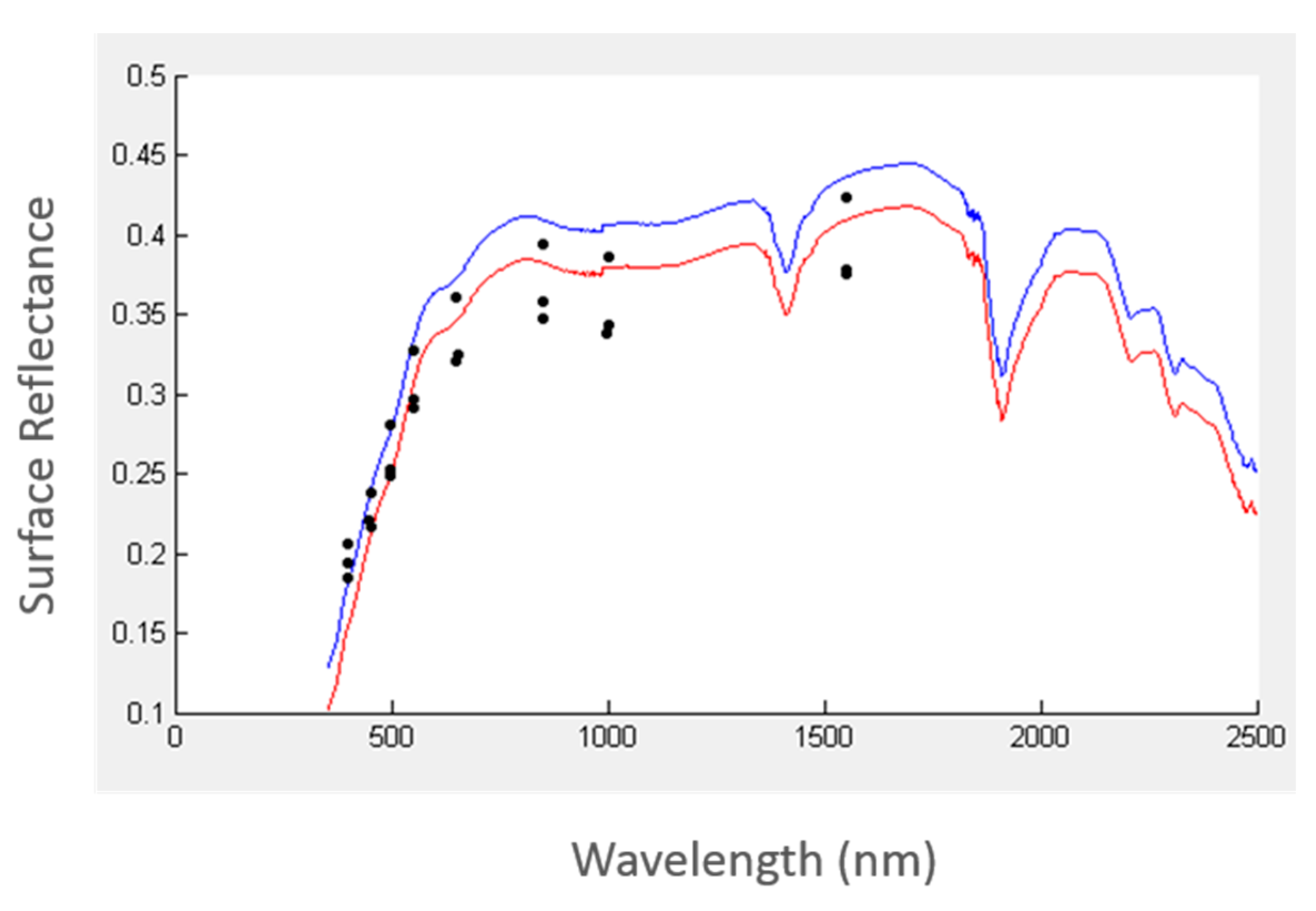
2.2.1. Surface Reflectance

| Band | Center Wavelength (nm) | Bandwidth (nm) |
|---|---|---|
| 1 | 400 | 20 |
| 2 | 450 | |
| 3 | 500 | |
| 4 | 550 | |
| 5 | 650 | |
| 6 | 850 | |
| 7 | 1000 | |
| 8 | 1550 |
- The band-averaged surface BRF is determined for each channel of every GVR using Equation (1).
- The band-averaged BRF of the entire 1-km2 site in each of the eight GVR channels is determined by averaging the individual GVR measurements for each channel.
- A reference spectra of hyperspectral data is chosen from a library of Railroad Valley BRF spectra.
- The chosen reference spectra is fit to the average BRF using a least squares fit, which produces a hyperspectral BRF for the date and time of interest.
2.2.2. Atmospheric Measurements

2.2.3. Top-of-Atmosphere Spectral Radiance and Reflectance
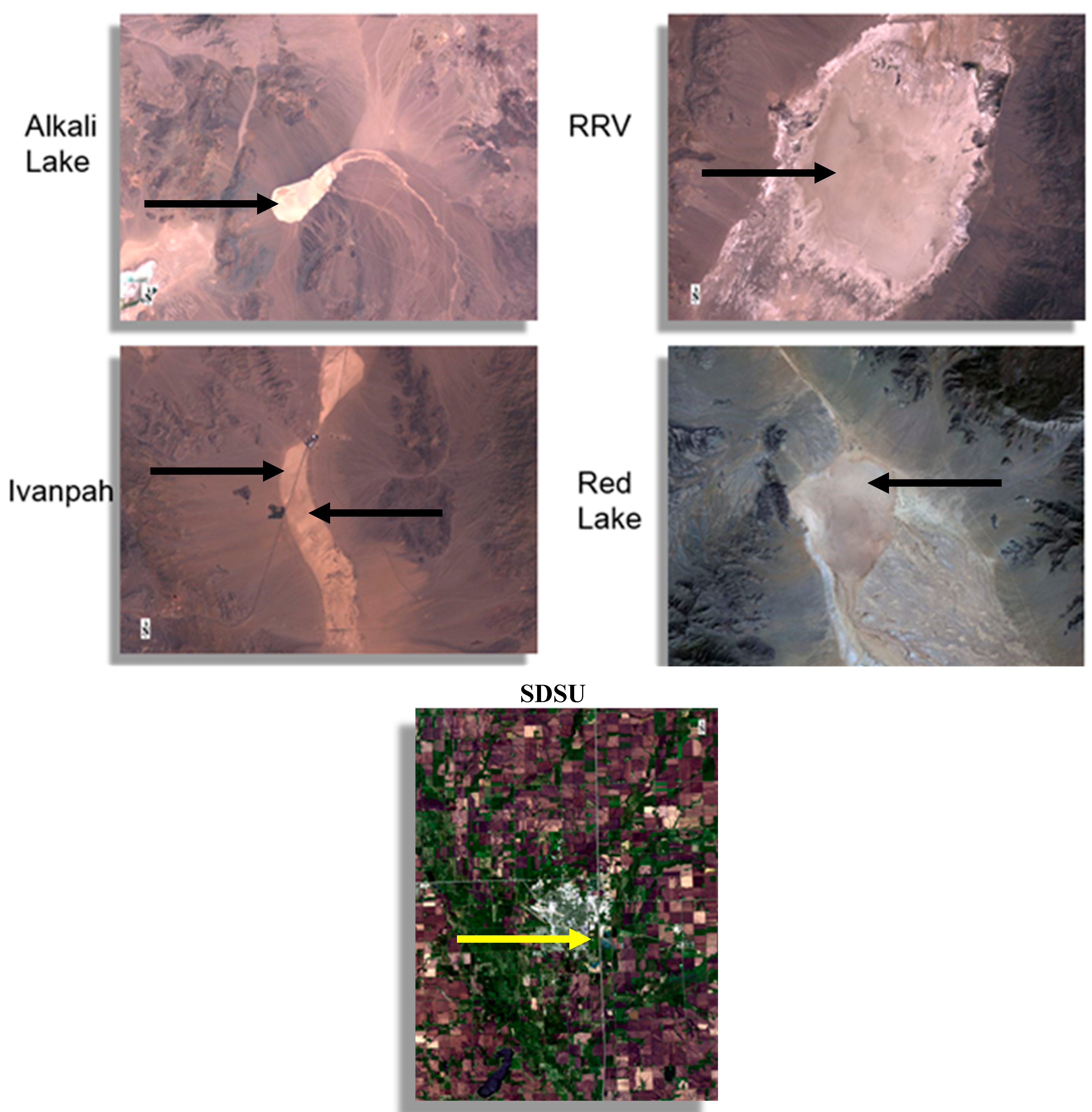
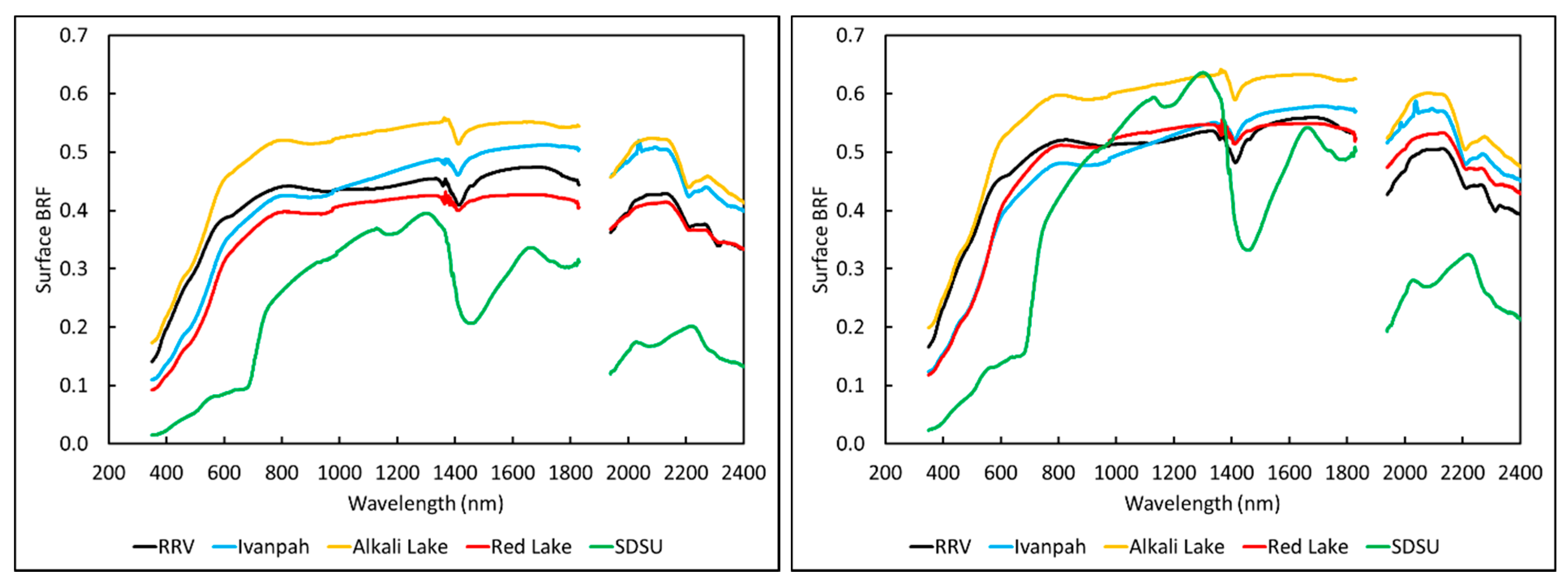
3. Data
3.1. Reflectance-Based Approach and Cross Calibration with ETM+
| Date (yyyy-mm-dd) | 2013-03-19 | 2013-03-24 | 2013-03-29 | 2013-04-20 | 2013-04-29 | 2013-10-15 | 2013-11-14 | 2014-02-04 | 2014-03-08 | 2014-05-09 |
|---|---|---|---|---|---|---|---|---|---|---|
| Site (Team) | Railroad Valley (UA) | Ivanpah Playa (UA, GSFC) | Red Lake (UA, GSFC) | Railroad Valley (UA) | Ivanpah Playa (UA) | Red Lake (UA) | Railroad Valley (UA) | Red Lake (UA) | Red Lake (UA) | Railroad Valley (UA) |
| Collection area (m) | 90 × 500 | 120 × 300 | 120 × 300 | 90 × 500 | 120 × 300 | 120 × 300 | 90 × 500 | 120 × 300 | 120 × 300 | 90 × 500 |
| Time (UTC) | 18:19:54 | 18:16:29 | 18:05:34 (L7) 18:12:12 (L8) | 18:22:47 | 18:17:26 | 18:11:03 | 18:22:47 | 18:10:33 | 18:09:55 | 18:20:38 |
| Solar zenith angle (degrees) | 44.0 | 40.0 | 38.9 (L7) 38.0 (L8) | 32.0 | 27.7 | 46.6 | 58.9 | 56.3 | 46.3 | 27.1 |
| Solar azimuth angle (degrees) | 146.4 | 142.8 | 140.0 (L7) 142.3 (L8) | 141.4 | 133.7 | 159.7 | 162.1 | 151.2 | 145.6 | 135.2 |
| Aerosol Optical Depth (550 nm) | 0.048 | 0.068 | 0.068 | 0.085 | 0.122 | 0.046 | 0.021 | 0.032 | 0.025 | 0.089 |
| Ozone (DU) | 298 | 296 | 306 | 309 | 323 | 286 | 326 | 333 | 311 | 356 |
| Water vapor (cm) | 1.19 | 0.77 | 1.64 | 1.10 | 1.24 | 0.77 | 0.58 | 0.82 | 0.60 | 1.21 |
| Temperature (°C) | 14.1 | 16.4 | 25.1 | 15.5 | 33.9 | 18.8 | 10.3 | 9.0 | 18.4 | 20.5 |
| Pressure (mb) | 859.3 | 926.7 | 922.8 | 859.5 | 919.0 | 919.8 | 859.2 | 920.0 | 925.6 | 853.1 |
| Satellite Information | ||||||||||
| View zenith angle (degrees) | 4.6 | 4.3 | 5.4 (L7) 2.7 (L8) | 0.8 | 3.7 | 5.9 | 0.3 | 5.1 | 5.5 | 0.3 |
| View azimuth angle (degrees) | 102.6 | 103.1 | 101.9 (L7) 100.7 (L8) | 95.0 | 96.9 | 101.7 | 122.6 | 100.5 | 95.1 | 148.9 |
| Date (yyyy-mm-dd) | 2013-03-30 | 2013-06-10 | 2013-07-12 | 2013-08-13 | 2013-08-29 | 2013-09-30 | 2013-10-16 |
|---|---|---|---|---|---|---|---|
| Site (Team) | SDSU Test Site (SDSU) | SDSU Test Site (SDSU) | SDSU Test Site (SDSU) | SDSU Test Site (SDSU) | SDSU Test Site (SDSU) | SDSU Test Site (SDSU) | SDSU Test Site (SDSU) |
| Collection area (m) | 100 × 250 | 100 × 250 | 100 × 250 | 100 × 250 | 100 × 250 | 100 × 250 | 100 × 250 |
| Time (UTC) | 17:07:14 (L7) 17:09:43 (L8) | 17:13:23 | 17:13:22 | 17:13:23 | 17:13:25 | 17:13:15 | 17:13:14 |
| Solar zenith angle (degrees) | 43.9 | 26.0 | 27.8 | 34.2 | 38.8 | 49.5 | 55.2 |
| Solar azimuth angle (degrees) | 151.3 | 139.2 | 137.8 | 145.0 | 150.0 | 159.1 | 162.2 |
| Aerosol Optical Depth (550 nm) | 0.158 | 0.060 | 0.183 | 0.195 | 0.067 | 0.016 | 0.077 |
| Ozone (DU) | 324 | 287 | 290 | 291 | 289 | 284 | 279 |
| Water vapor (cm) | 0.53 | 2.76 | 1.76 | 2.93 | 2.64 | 2.01 | 3.02 |
| Temperature (°C) | 7.2 | 18.9 | 27.8 | 21.7 | 31.0 | 22.5 | 8.9 |
| Pressure (mb) | 951.9 | 947.9 | 948.9 | 956.7 | 945.5 | 936.0 | 954.6 |
| Satellite Information | |||||||
| View zenith angle (degrees) | 0.1 (L7) 5.0 (L8) | 0.1 | 0.3 | 0.3 | 0.2 | 0.3 | 0.2 |
| View azimuth angle (degrees) | 278.9 (L7) 278.9 (L8) | 278.9 | 278.9 | 278.9 | 278.9 | 278.9 | 278.9 |
3.2. RadCaTS
| Date (yyyy-mm-dd) | 2013-05-22 | 2013-06-07 | 2013-06-23 | 2013-08-10 | 2013-11-14 |
|---|---|---|---|---|---|
| Site | Railroad Valley | Railroad Valley | Railroad Valley | Railroad Valley | Railroad Valley |
| Collection area (m) | 1000 × 1000 | 1000 × 1000 | 1000 × 1000 | 1000 × 1000 | 1000 × 1000 |
| Time (UTC) | 18:23:06 | 18:23:03 | 18:22:54 | 18:22:49 | 18:22:47 |
| Solar zenith angle (degrees) | 24.4 | 23.0 | 23.1 | 29.8 | 58.9 |
| Solar azimuth angle (degrees) | 132.1 | 127.4 | 124.8 | 135.1 | 162.1 |
| Aerosol Optical Depth (550 nm) | 0.062 | 0.051 | 0.044 | 0.042 | 0.019 |
| OMI Ozone (DU) | 335 | 300 | 323 | 311 | 286 |
| Water vapor (cm) | 0.75 | 0.84 | 0.87 | 0.83 | 0.41 |
| Temperature (°C) | 25.0 | 32.5 | 27.8 | 27.8 | 8.8 |
| Pressure (mb) | 845 | 857 | 851 | 858 | 860 |
| Satellite Information | |||||
| View zenith angle (degrees) | 0.2 | 0.3 | 0.7 | 0.9 | 0.3 |
| View azimuth angle (degrees) | 85.2 | 76.0 | 100.0 | 91.7 | 122.6 |
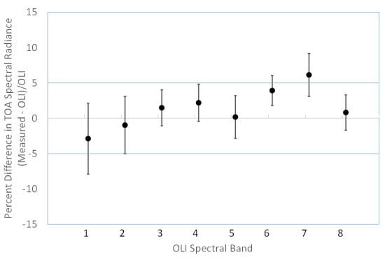
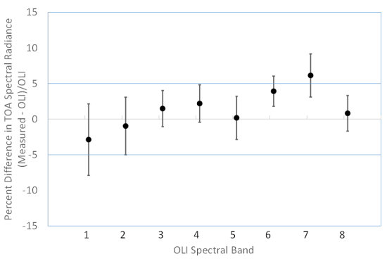
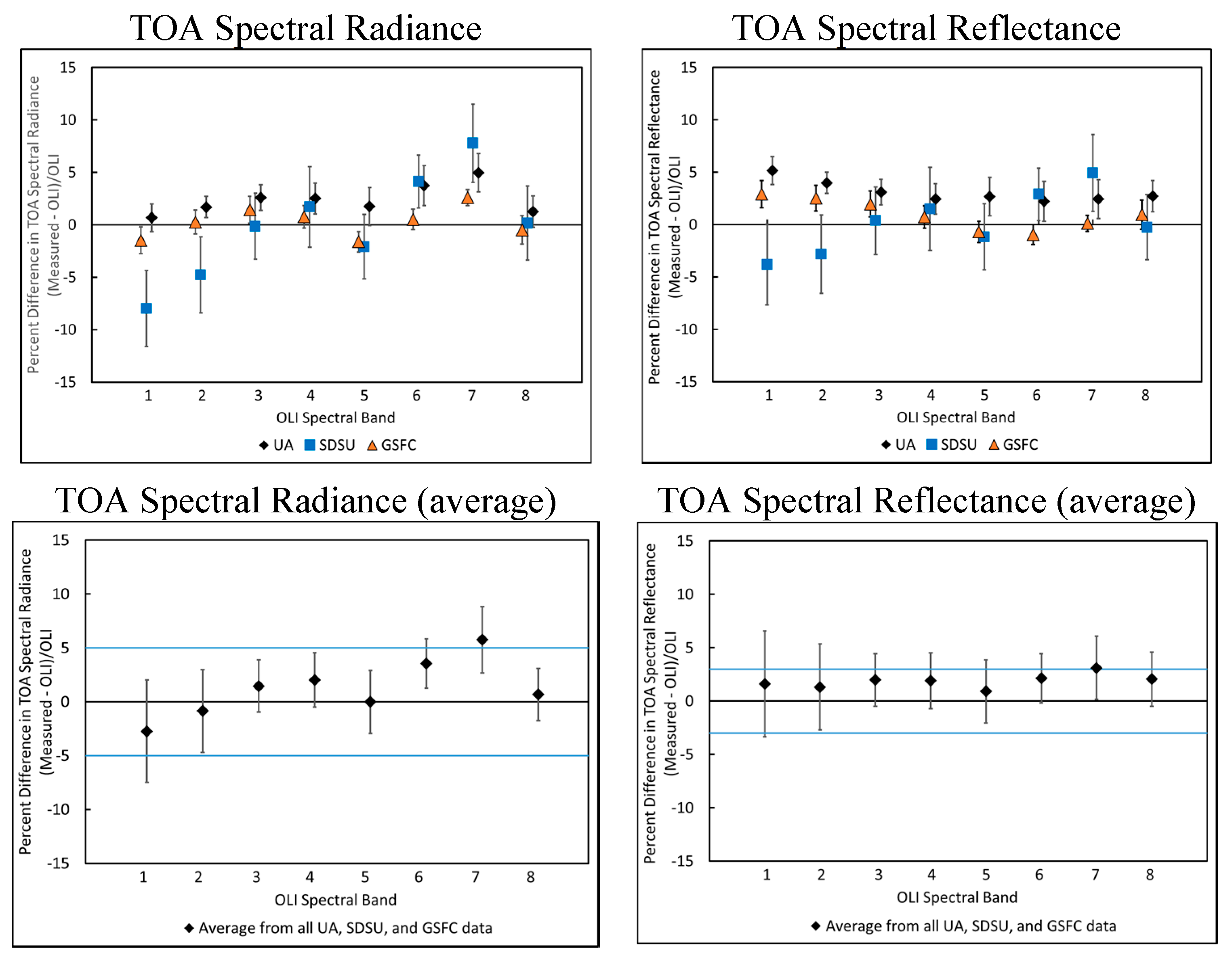
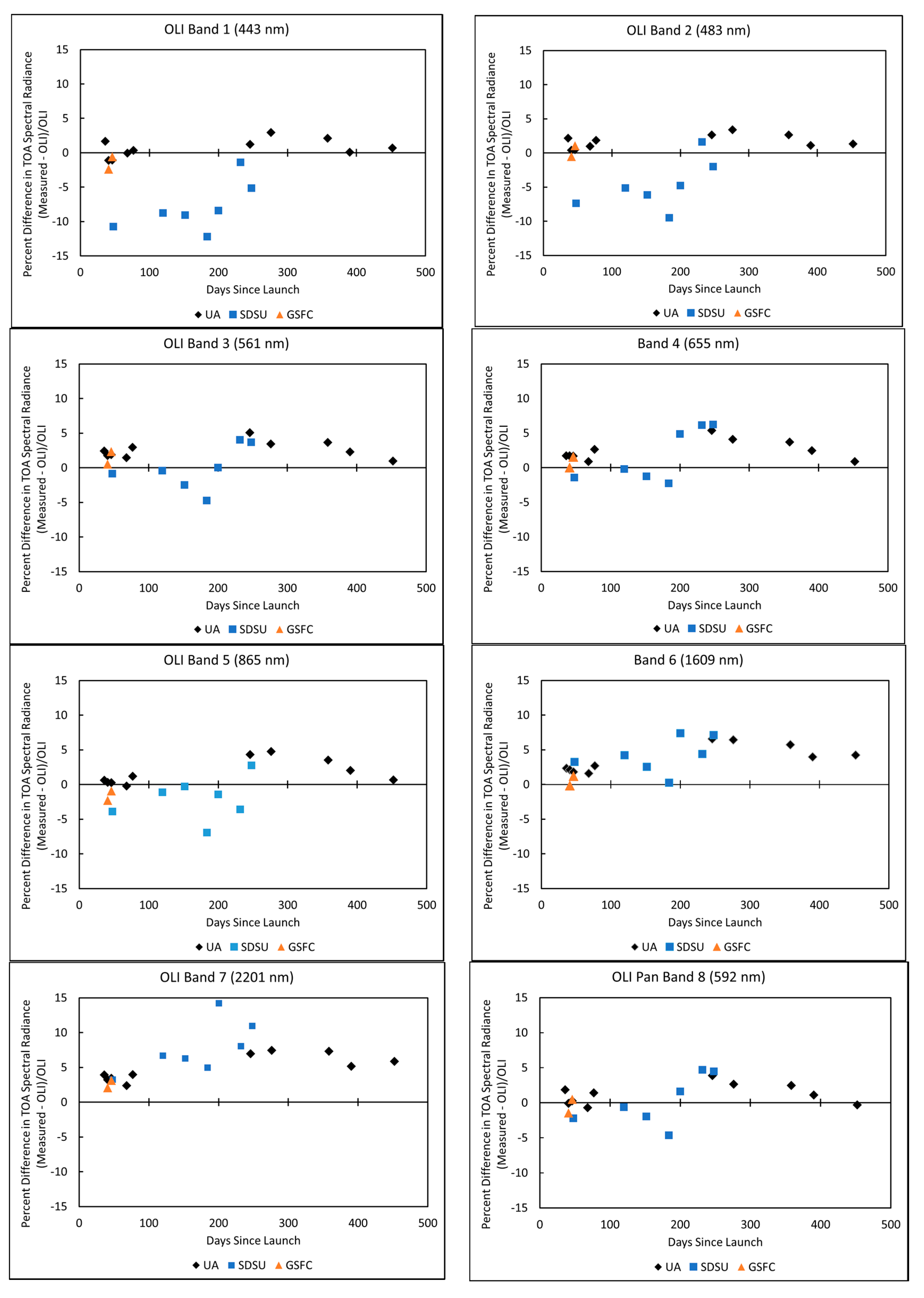
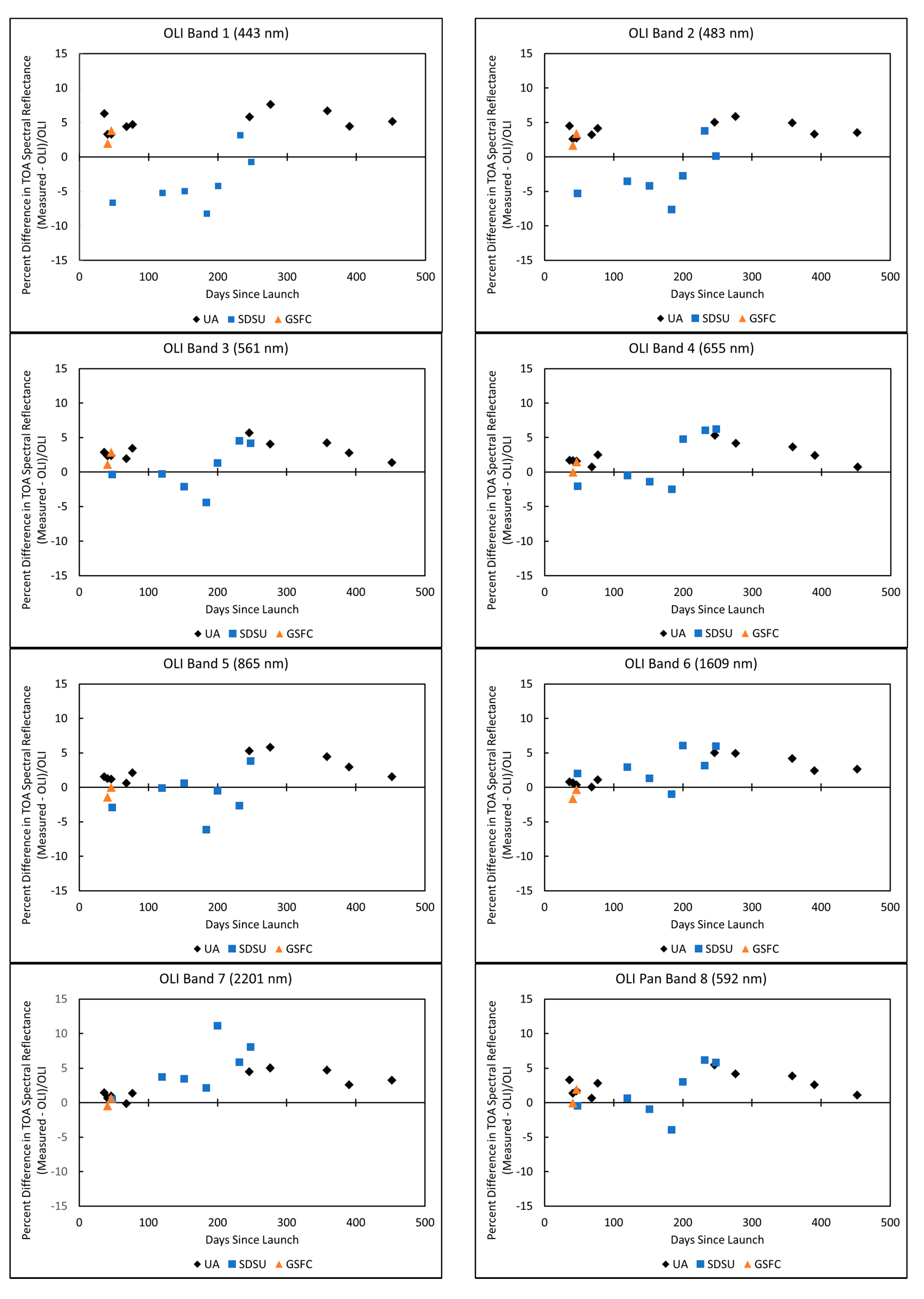
4. Results
4.1. Reflectance-Based Results


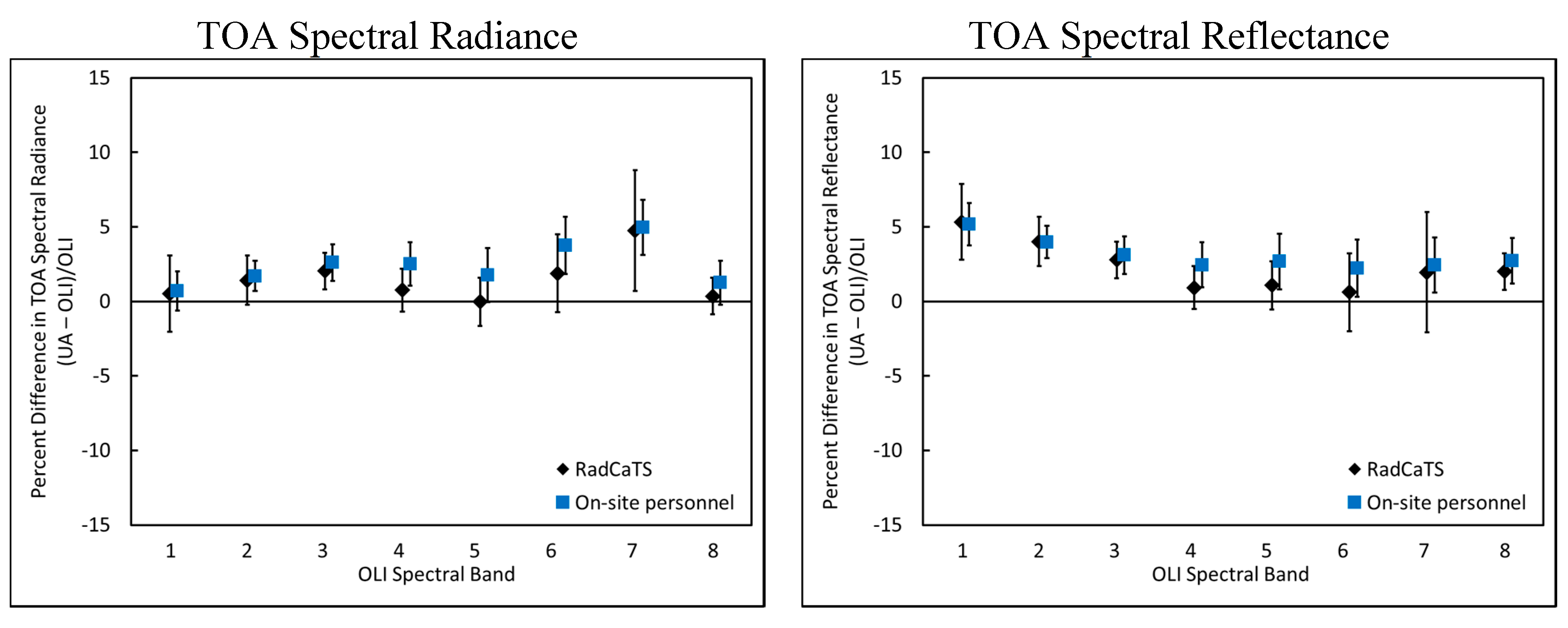
4.2. RadCaTS Results

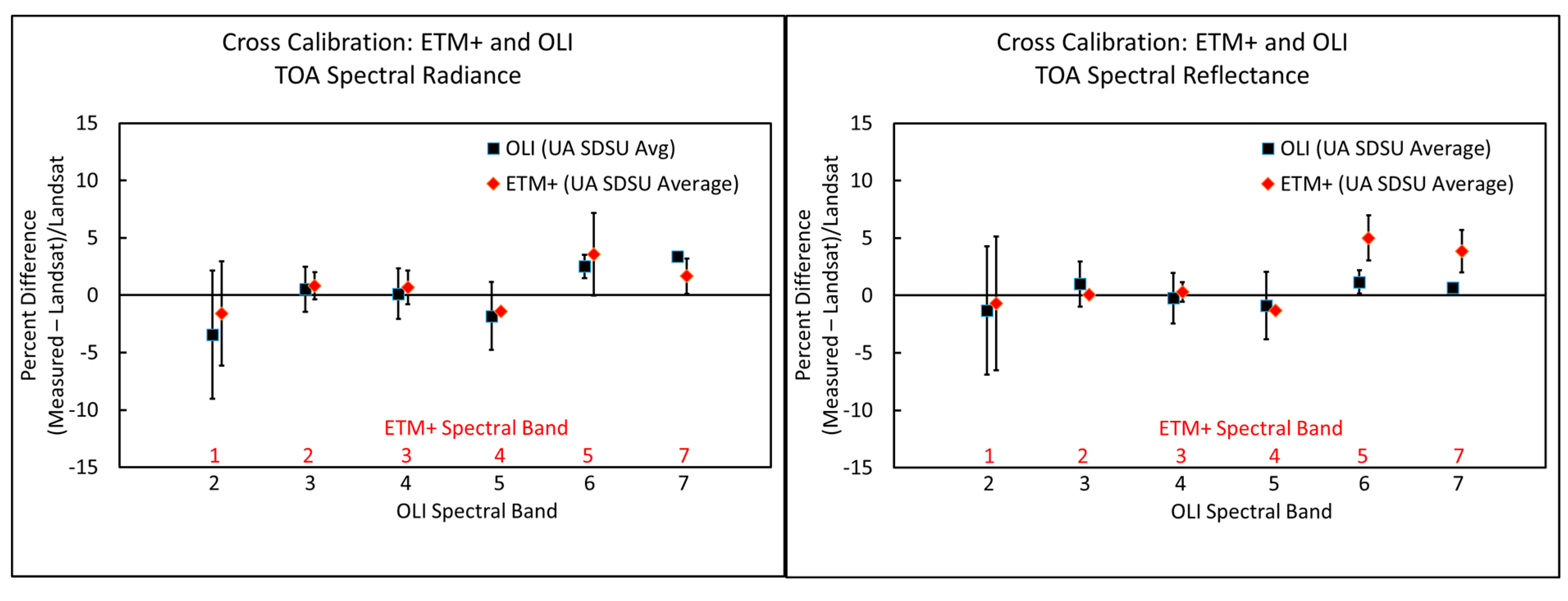
4.3. Landsat 7 ETM+ and Landsat 8 OLI Cross Comparison Results

5. Uncertainty Analysis
5.1. Reflectance-Based Approach
| Source of Uncertainty | Source | TOA Spectral Radiance |
|---|---|---|
| Ground reflectance measurement | 1.6% | |
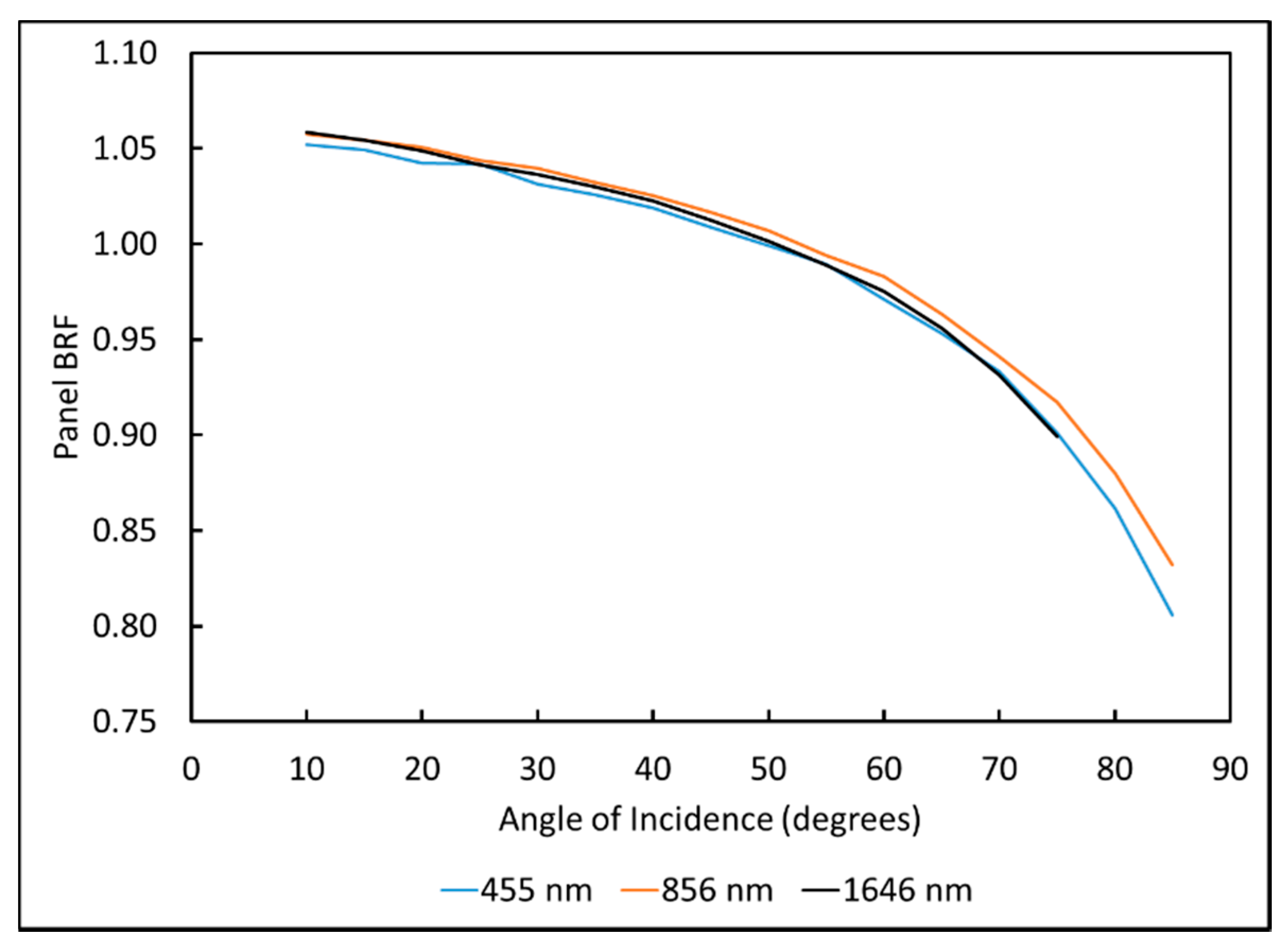
| Reference panel calibration (BRF) | 1.3% | |
| Site measurement errors | 1.0% | |
| Optical depth measurements | 0.5% | <0.1% |
| Extinction optical depth | 0.5% | |
| Absorption computations | --- | |
| Column ozone (OMI) | 3.0% | |
| Column water vapor | 5.0% | |
| Choice of aerosol complex index | 100% | 0.5% |
| Choice of aerosol size distribution | 0.3% | |
| Junge parameter | 0.3% | |
| Non-lambertian surface | 10% | --- |
| Other | ||
| Non-polarization vs. polarization | 0.1% | |
| Inherent accuracy of MODTRAN 5 | 2.0% | |
| Uncertainty in solar zenith angle | 0.2% | |
| Total RSS uncertainty | 2.6% |
5.2. RadCaTS
- (1)
- Radiometric calibration of the GVRs.
- (2)
- The radiative transfer code uncertainty, which includes:
- (a)
- Uncertainty in the solar irradiance model.
- (b)
- Atmospheric transmission.
- (c)
- Determination of the diffuse sky irradiance.
- (3)
- Surface BRF retrieval, which includes uncertainties introduced by scaling the hyperspectral reference BRF data with point measurements from the GVRs.
| Source of Uncertainty | Surface BRF Uncertainty | |||
|---|---|---|---|---|
| GVR Band | ||||
| 450 nm | 650 nm | 850 nm | 1550 nm | |
| Individual GVR measurement | 2.7% | 2.4% | 2.5% | 2.2% |
| Scaling hyperspectral reference data | 2.6% | 1.7% | 2.8% | 3.3% |
| Total BRF uncertainty | 3.7% | 2.9% | 3.8% | 4.0% |
RadCaTS Uncertainty Results
| RadCaTS TOA Spectral Radiance Uncertainty | |||
|---|---|---|---|
| GVR Band | |||
| 450 nm | 650 nm | 850 nm | 1550 nm |
| 4.1% | 3.1% | 4.1% | 4.1% |
6. Conclusions
Acknowledgements
Author Contributions
Conflicts of Interest
References
- Reuter, D.; Richardson, C.; Irons, J.; Allen, R.; Anderson, M.; Budinoff, J.; Casto, G.; Coltharp, C.; Finneran, P.; Forsbacka, B.; et al. The Thermal Infrared Sensor on the Landsat Data Continuity Mission. In Proceedings of 2010 IEEE International Geoscience and Remote Sensing Symposium (IGARSS), Honolulu, HI ,USA, 25–30 July 2010.
- Reuter, D.; Richardson, C.; Pellerano, F.; Irons, J.; Allen, R.; Anderson, M.; Jhabvala, M.; Lunsford, A.; Montanaro, M.; Smith, R.; et al. The Thermal Infrared Sensor (TIRS) on Landsat 8: Design overview and pre-launch characterization. Remote Sens. 2015, 7. in press. [Google Scholar]
- Ungar, S.G.; Pearlman, J.S.; Mendenhall, J.A.; Reuter, D. Overview of the Earth Observing One (EO-1) mission. IEEE Trans. Geosci. Remote Sens. 2003, 41, 1149–1159. [Google Scholar] [CrossRef]
- Irons, J.R.; Dwyer, J.L.; Barsi, J.A. The next Landsat satellite: The Landsat Data Continuity Mission. Remote Sens. Environ. 2012, 122, 11–21. [Google Scholar] [CrossRef]
- Markham, B.; Barsi, J.; Kvaran, G.; Ong, L.; Kaita, E.; Biggar, S.; Czapla-Myers, J.; Mishra, N.; Helder, D. Landsat-8 operational land imager radiometric calibration and stability. Remote Sens. 2014, 6, 12275–12308. [Google Scholar] [CrossRef]
- Kuester, M.A.; Czapla-Myers, J.; Kaptchen, P.; Good, W.; Lin, T.; To, R.; Biggar, S.; Thome, K. Development of a heliostat facility for solar-radiation-based calibration of earth observing sensors. In Proceedings of Earth Observing Systems XIII, San Diego, CA, USA, 28 August 2008.
- Czapla-Myers, J.; Thome, K.; Anderson, N.; McCorkel, J.; Leisso, N.; Good, W.; Collins, S. Transmittance measurement of a heliostat facility used in the preflight radiometric calibration of Earth-observing sensors. In Proceedings of SPIE Optics and Photonics 2009, San Diego, CA, USA, 2–6 August 2009.
- Knight, E.; Kvaran, G. Landsat-8 operation land imager design, characterization and performance. Remote Sens. 2014, 6, 10286–10305. [Google Scholar] [CrossRef]
- Slater, P.N.; Biggar, S.F.; Holm, R.G.; Jackson, R.D.; Mao, Y.; Moran, M.S.; Palmer, J.M.; Yuan, B. Reflectance- and radiance-based methods for the in-flight absolute calibration of multispectral sensors. Remote Sens. Environ. 1987, 22, 11–37. [Google Scholar] [CrossRef]
- Teillet, P.M.; Slater, P.N.; Ding, Y.; Santer, R.P.; Jackson, R.D.; Moran, M.S. Three methods for the absolute calibration of the NOAA AVHRR sensors in-flight. Remote Sens. Environ. 1990, 31, 105–120. [Google Scholar] [CrossRef]
- Thome, K.J.; Crowther, B.G.; Biggar, S.F. Reflectance- and irradiance-based calibration of Landsat 5 thematic mapper. Can. J. Remote Sens. 1997, 23, 309–317. [Google Scholar] [CrossRef]
- Thome, K.J. Absolute radiometric calibration of Landsat 7 ETM+ using the reflectance-based method. Remote Sens. Environ. 2001, 78, 27–38. [Google Scholar] [CrossRef]
- Thome, K.J.; Biggar, S.F.; Choi, H.J. Vicarious calibration of Terra ASTER, MISR, and MODIS. In Proceedings of Earth Observing Systems IX, Denver, CO, USA, 26 October 2004.
- Thome, K.J.; Arai, K.; Tsuchida, S.; Biggar, S.F. Vicarious calibration of ASTER via the reflectance-based approach. IEEE Trans. Geosci. Remote Sens. 2008, 46, 3285–3295. [Google Scholar] [CrossRef]
- Naughton, D.; Brunn, A.; Czapla-Myers, J.; Douglass, S.; Thiele, M.; Weichelt, H.; Oxfort, M. Absolute radiometric calibration of the RapidEye Multi-Spectral Imager using the reflectance based vicarious calibration method. J. Appl. Remote Sens. 2011, 5. [Google Scholar] [CrossRef]
- Jackson, R.D.; Moran, M.S.; Slater, P.N.; Biggar, S.F. Field calibration of reference reflectance panels. Remote Sens. Environ. 1987, 22, 145–158. [Google Scholar] [CrossRef]
- Biggar, S.F.; Labed, J.F.; Santer, R.P.; Slater, P.N.; Jackson, R.D.; Moran, M.S. Laboratory calibration of field reflectance panels. In Proceedings of Recent Advances in Sensors, Radiometry, and Data Processing for Remote Sensing, Orlando, FL, USA, 6–8 April 1988.
- Anderson, N.J.; Biggar, S.F.; Burkhart, C.; Thome, K.J.; Mavko, M.E. Bi-directional calibration results for the cleaning of spectralon reference panels. In Proceedings of Earth Observing Systems VII, Seattle, WA, USA, 24 September 2002.
- Helder, D.; Thome, K.; Aaron, D.; Leigh, L.; Czapla-Myers, J.; Leisso, N.; Biggar, S.; Anderson, N. Recent surface reflectance measurement campaigns with emphasis on best practices, SI traceability and uncertainty estimation. Metrologia 2012, 49. [Google Scholar] [CrossRef]
- Ehsani, A.R.; Reagan, J.A.; Erxleben, W.H. Design and performance analysis of an automated 10-channel solar radiometer instrument. J. Atmos. Oceanic Technol. 1998, 15, 697–707. [Google Scholar] [CrossRef]
- Biggar, S.F.; Gellman, D.I.; Slater, P.N. Improved evaluation of optical depth components from langley plot data. Remote Sens. Environ. 1990, 32, 91–101. [Google Scholar] [CrossRef]
- Biggar, S.F.; Slater, P.N.; Gellman, D.I. Uncertainties in the in-flight calibration of sensors with reference to measured ground sites in the 0.4–1.1 μm range. Remote Sens. Environ. 1994, 48, 245–252. [Google Scholar] [CrossRef]
- Reagan, J.A.; Thome, K.J.; Herman, B.M. A Simple Instrument and Technique for Measuring Columnar Water Vapor via Near-IR Differential Solar Transmission Measurments. In Proceedings of Geoscience and Remote Sensing Symposium, 1991, IGARSS’91. Espo, Finland, 3–6 Jun 1991; Remote Sensing: Global Monitoring for Earth Management, International.
- Thome, K.J.; Smith, M.W.; Palmer, J.M.; Reagan, J.A. Three-channel solar radiometer for the determination of atmospheric columnar water vapor. Appl. Opt. 1994, 33, 5811–5819. [Google Scholar] [CrossRef] [PubMed]
- Thome, K.J.; Helder, D.L.; Aaron, D.; Dewald, J.D. Landsat-5 TM and Landsat-7 ETM+ absolute radiometric calibration using the reflectance-based method. IEEE Trans. Geosci. Remote Sens. 2004, 42, 2777–2785. [Google Scholar] [CrossRef]
- Berk, A.; Anderson, G.P.; Acharya, P.K.; Shettle, E.P. MODTRAN 5.2.1 User’s Manual; Spectral Sciences Inc.,Air Force Research Laboratory: Burlington, MA, USA and Hanscom AFB, MA, USA, 2011. [Google Scholar]
- Holben, B.N.; Eck, T.F.; Slutsker, I.; Tanré, D.; Buis, J.P.; Setzer, A.; Vermote, E.; Reagan, J.A.; Kaufman, Y.J.; Nakajima, T.; Lavenu, F.; Janjowiak, I.; Smirnov, A. AERONET—A federated instrument network and data archive for aerosol characterization. Remote Sens. Environ. 1998, 66, 1–16. [Google Scholar] [CrossRef]
- Anderson, N.J.; Czapla-Myers, J.S. Ground viewing radiometer characterization, implementation and calibration applications: A summary after two years of field deployment. In Proceedings of Earth Observing Systems XVIII, San Diego, CA, USA, 23 September 2013.
- Anderson, N.; Czapla-Myers, J.; Leisso, N.; Biggar, S.; Burkhart, C.; Kingston, R.; Thome, K. Design and calibration of field deployable ground-viewing radiometers. Appl. Opt. 2013, 52, 231–240. [Google Scholar] [CrossRef] [PubMed]
- Thome, K.; Smith, N.; Scott, K. Vicarious calibration of MODIS using Railroad Valley Playa. In Proceedings of International Geoscience and Remote Sensing Symposium 2001 (IGARSS), Sydney, Australia, 9–13 July 2001.
- Thome, K.; D’Amico, J.; Hugon, C. Intercomparison of Terra ASTER, MISR, and MODIS, and Landsat-7 ETM+. In Proceedings of IEEE International Conference on Geoscience and Remote Sensing Symposium, IGARSS 2006, Denver, CO, USA, 31 July–4 August 2006.
- Czapla-Myers, J.S.; Thome, K.J.; Leisso, N.P. Calibration of AVHRR sensors using the reflectance-based method. In Proceedings of Atmospheric and Environmental Remote Sensing Data Processing and Utilization III: Readiness for GEOSS, San Diego, CA, USA, 24 September 2007.
- Leisso, N.; Czapla-Myers, J. Comparison of diffuse sky irradiance calculation methods and effect on surface reflectance retrieval from an automated radiometric calibration test site. In Proceedings of Earth Observing Systems XVI, San Diego, CA, USA, 14 September 2011.
- Cook, B.D.; Corp, L.A.; Nelson, R.F.; Middleton, E.M.; Morton, D.C.; McCorkel, J.T.; Masek, J.G.; Ranson, K.J.; Vuong, L.; Montesano, P.M. NASA Goddard’s LiDAR, Hyperspectral and Thermal (G-LiHT) airborne imager. Remote Sens. 2013, 5, 4045–4066. [Google Scholar] [CrossRef]
- Slater, P.N.; Biggar, S.F.; Thome, K.J.; Gellman, D.I.; Spyak, P.R. Vicarious radiometric calibrations of EOS sensors. J. Atmos. Oceanic Technol. 1996, 13, 349–359. [Google Scholar] [CrossRef]
- Thome, K.; Cattrall, C.; D’Amico, J.; Geis, J. Ground-reference calibration results for Landsat-7 ETM+. In Proceedings of Earth Observing Systems X, San Diego, CA, USA, 7 September 2005.
- Thuillier, G.; Hersé, M.; Simon, P.; Labs, D.; Mandel, H.; Gillotay, D.; Foujols, T. The visible solar spectral irradiance from 350 to 850 nm as measured by the solspec spectrometer during the Atlas I Mission. In Solar Electromagnetic Radiation Study for Solar Cycle 22; Pap, J.M., Fröhlich, C., Ulrich, R.K., Eds.; Springer: Berlin, Germany, 1998; pp. 41–61. [Google Scholar]
- Thuillier, G.; Hersé, M.; Labs, D.; Foujols, T.; Peetermans, W.; Gillotay, D.; Simon, P.C.; Mandel, H. The solar spectral irradiance from 200 to 2400 nm as measured by the SOLSPEC spectrometer from the Atlas and Eureca Missions. Sol. Phys. 2003, 214, 1–22. [Google Scholar] [CrossRef]
- Bhartia, P.K. OMI algorithm theoretical basis document. Volume II. OMI Ozone Products. Available online: eospso.gsfc.nasa.gov/sites/default/files/atbd/ATBD-OMI-02.pdf (accessed on 1 August 2014).
- Czapla-Myers, J.S.; Thome, K.J.; Buchanan, J.H. Implication of spatial uniformity on vicarious calibration using automated test sites. In Proceedings of Earth Observing Systems XII, San Diego, CA, USA, 27 September 2007.
- Czapla-Myers, J.S.; Thome, K.J.; Cocilovo, B.R.; McCorkel, J.T.; Buchanan, J.H. Temporal, spectral, and spatial study of the automated vicarious calibration test site at Railroad Valley, Nevada. In Proceedings of Earth Observing Systems XIII, San Diego, CA, USA, 20 August 2008.
© 2015 by the authors; licensee MDPI, Basel, Switzerland. This article is an open access article distributed under the terms and conditions of the Creative Commons Attribution license (http://creativecommons.org/licenses/by/4.0/).
Share and Cite
Czapla-Myers, J.; McCorkel, J.; Anderson, N.; Thome, K.; Biggar, S.; Helder, D.; Aaron, D.; Leigh, L.; Mishra, N. The Ground-Based Absolute Radiometric Calibration of Landsat 8 OLI. Remote Sens. 2015, 7, 600-626. https://doi.org/10.3390/rs70100600
Czapla-Myers J, McCorkel J, Anderson N, Thome K, Biggar S, Helder D, Aaron D, Leigh L, Mishra N. The Ground-Based Absolute Radiometric Calibration of Landsat 8 OLI. Remote Sensing. 2015; 7(1):600-626. https://doi.org/10.3390/rs70100600
Chicago/Turabian StyleCzapla-Myers, Jeffrey, Joel McCorkel, Nikolaus Anderson, Kurtis Thome, Stuart Biggar, Dennis Helder, David Aaron, Larry Leigh, and Nischal Mishra. 2015. "The Ground-Based Absolute Radiometric Calibration of Landsat 8 OLI" Remote Sensing 7, no. 1: 600-626. https://doi.org/10.3390/rs70100600