Article

Adjusting Lidar-Derived Digital Terrain Models in Coastal Marshes Based on Estimated Aboveground Biomass Density

1
Department of Civil, Environmental and Construction Engineering, University of Central Florida, 12800 Pegasus Drive, Suite 211., Orlando, FL 32816, USA
2
Department of Civil & Environmental Engineering, Center for Computation and Technology, Louisiana State University, 3418 Patrick F. Taylor, Baton Rouge, LA 70803, USA
3
Department of Biology, University of Central Florida, 4110 Libra Drive, Orlando, FL 32816, USA
4
Sandia National Laboratories, P.O. Box 5800, MS 1163, Albuquerque, NM 87185, USA
*
Author to whom correspondence should be addressed.
Remote Sens. 2015, 7(4), 3507-3525; https://doi.org/10.3390/rs70403507
Submission received: 5 December 2014 / Revised: 10 March 2015 / Accepted: 17 March 2015 / Published: 25 March 2015
(This article belongs to the Special Issue Towards Remote Long-Term Monitoring of Wetland Landscapes)

Abstract

:
Digital elevation models (DEMs) derived from airborne lidar are traditionally unreliable in coastal salt marshes due to the inability of the laser to penetrate the dense grasses and reach the underlying soil. To that end, we present a novel processing methodology that uses ASTER Band 2 (visible red), an interferometric SAR (IfSAR) digital surface model, and lidar-derived canopy height to classify biomass density using both a three- class scheme (high, medium and low) and a two-class scheme (high and low). Elevation adjustments associated with these classes using both median and quartile approaches were applied to adjust lidar-derived elevation values closer to true bare earth elevation. The performance of the method was tested on 229 elevation points in the lower Apalachicola River Marsh. The two-class quartile-based adjusted DEM produced the best results, reducing the RMS error in elevation from 0.65 m to 0.40 m, a 38% improvement. The raw mean errors for the lidar DEM and the adjusted DEM were 0.61 ± 0.24 m and 0.32 ± 0.24 m, respectively, thereby reducing the high bias by approximately 49%.

Graphical Abstract

1. Introduction

Tidal salt marshes are among the most complex and productive ecosystems in the world [1,2]. Occurring at the interface between terrestrial and aquatic ecosystems and often between saline and non-saline water bodies, they provide valuable ecological services such as nutrient cycling, pollutant filtration, floodwater absorption, storm surge dissipation, and shoreline stabilization [2,3]. Salt marshes have some of the highest levels of net primary production, with aboveground biomass production from marsh grasses of up to 4000 g∙m−2∙yr−1 and below-ground production estimated at over 6000 g∙m−2∙yr−1 in inland areas [4]. These high rates of primary production, in turn, support a diverse meso- and macrofauna including large populations of migratory waterfowl and wading birds and economically important species of fish and shellfish [2]. In addition to the tangible economic benefits from commercial fisheries, salt marshes provide a variety of other ecosystem services such as birdwatching, fishing, and other forms of recreation and tourism [3].
Despite their enormous value, salt marshes worldwide have been degraded or destroyed by a variety of anthropogenic threats including eutrophication due to agricultural and industrial runoff, drainage and reclamation for residential and commercial development, modification of hydrological flow regimes, relative sea level rise, increased air and water surface temperatures, and higher acidification associated with elevated atmospheric CO2 [1,5,6]. In the northern Gulf of Mexico, coastal marshes are threatened by accelerating submergence due to the loss of upstream sediments combined with rising sea levels [4]. In addition to rapid shoreline retreat from long-term coastal erosion, subsidence has led to the loss of thousands of square kilometers of salt marsh in the northern Gulf of Mexico through conversion to open water [1]. Even more troubling, estimates for global sea level rise based on the most recently available data suggest that an increase of 1 m or more by the year 2100 is a strong possibility given the accelerating loss of the polar ice sheets [7,8,9,10]. If realized, these projected rates of sea level rise in excess of 10 mm∙yr−1 would cause substantial losses of coastal marsh areas in the northern Gulf of Mexico [11].
To monitor the status of salt marshes on global to regional scales, it is vital to develop accurate quantitative relationships between metrics derived from remotely sensed data and indicators of salt marsh productivity such as aboveground biomass. Previous studies established strong correlations between live biomass of the salt marsh grass Spartina alterniflora (smooth cordgrass) and the canopy radiance corresponding to the red and near-infrared (NIR) spectral bands captured by Landsat Thematic Mapper (TM) sensors, as well as vegetation indices derived from those spectral bands [12]. Zhang et al. [13] reported statistically significant relationships between spectral vegetation indices derived from Landsat TM imagery and various measures of salt marsh biomass collected in San Pablo Bay, California. Among the models considered, the simple vegetation index (i.e., the near-infrared band divided by the red band) explained the most variation in green fresh biomass, with an R2 value of 0.58 [13]. Jensen et al. [3] used sub-meter resolution color-infrared (CIR) aerial photography in conjunction with field samples of biomass collected from salt marsh areas in coastal South Carolina to develop linear regression models relating the CIR spectral data to aboveground biomass of S. alterniflora. They found the strongest relationship between biomass and the NIR band, with an R2 value of 0.70 for the model containing this variable.
One of the major limitations of using satellite or CIR imagery to estimate aboveground biomass is the so-called “saturation problem,” wherein optical/infrared sensors are unable to distinguish variations in green biomass in areas of dense vegetation canopies. This saturation occurs when the canopy closure and leaf area density reach a threshold (varies by vegetation type) beyond which the optical/infrared sensor cannot detect increasing levels of green biomass response [14,15]. To address this problem, it has been proposed that biomass estimation could be improved by combining imagery from optical/infrared sensors with data acquired from active remote sensors, such as radar and airborne laser scanning (ALS, commonly referred to as “lidar” (light detection and ranging)) [14,16]. These active sensors provide additional information about topography and/or vegetation height that could potentially improve the quantitative models developed to predict aboveground biomass and other vegetation characteristics. Waring et al. [14] argued that Landsat imagery could be combined with synthetic aperture radar (SAR) data to improve biomass estimation in areas of dense vegetation, and Moghaddam et al. [17] reported significant improvements in regression models relating foliage biomass to Landsat TM data when combined with airborne SAR data collected over old-growth coniferous forests in the Pacific Northwest. In their study of woodland, shrub, grass, and mixed vegetation ecosystems in the Canadian arctic, Chen et al. [18] found that, in all cases, regression models combining Landsat TM and JERS-1 SAR data explained more of the variation in aboveground biomass than models containing either data source alone. Another type of active remote sensing technology, interferometric synthetic aperture radar (InSAR or IfSAR), requires that two SAR images be acquired over the same geographic area from a pair of close-range antennas. Because IfSAR can correct for terrain effects on radar backscatter intensity, it can potentially improve biomass estimation [19].
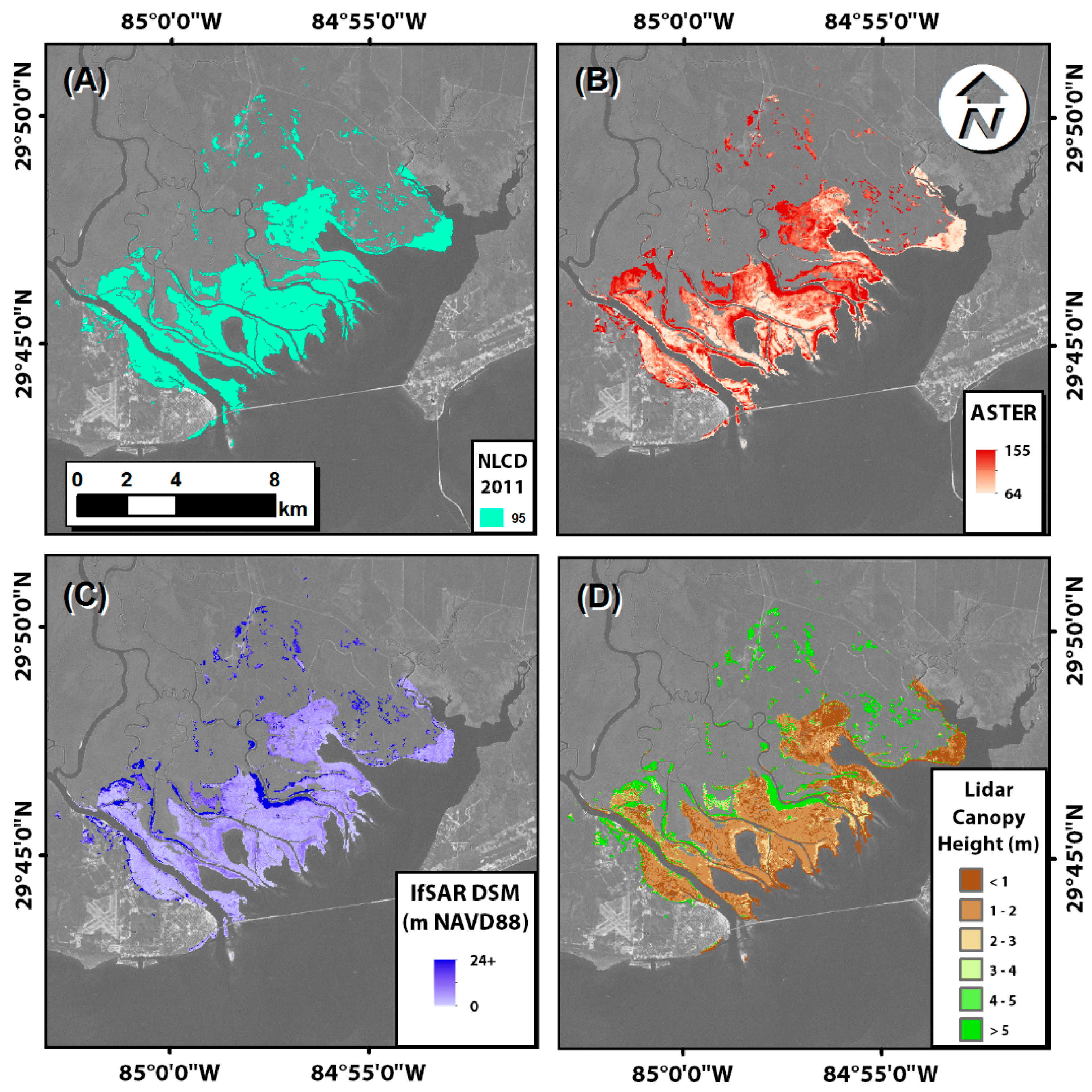
In recent years, lidar data have been used to estimate aboveground biomass and other biophysical parameters for a variety of forest, shrub, and grassland ecosystems [15,20]. More commonly, they have been used to develop digital terrain models for a variety of applications including coastal modeling [21]. However, it has been shown that the accuracy of lidar DEMs is reduced by vegetation, especially the tall, dense grasses typical of coastal salt marsh such as S. alterniflora and Juncus roemerianus (black rush) [22]. The term “lidar error” used herein is defined as the difference between the lidar DEM elevation and the true elevation at a specific location. This error has a significant impact on coastal modeling results in areas where dense vegetation degrades the accuracy of lidar-derived DEMs. In these areas the DEM estimates the elevation of the marsh platform (also known as the marsh table) on the order of 0.20 to 0.80 m above its true bare earth elevation. In terms of coastal modeling, this can prevent flooding of the marsh surface in a simulation under both normal tide and storm surge conditions. This has ramifications in engineering [23], ecological [24], and integrated models assessing major processes such as sea level rise and climate change [25,26,27].
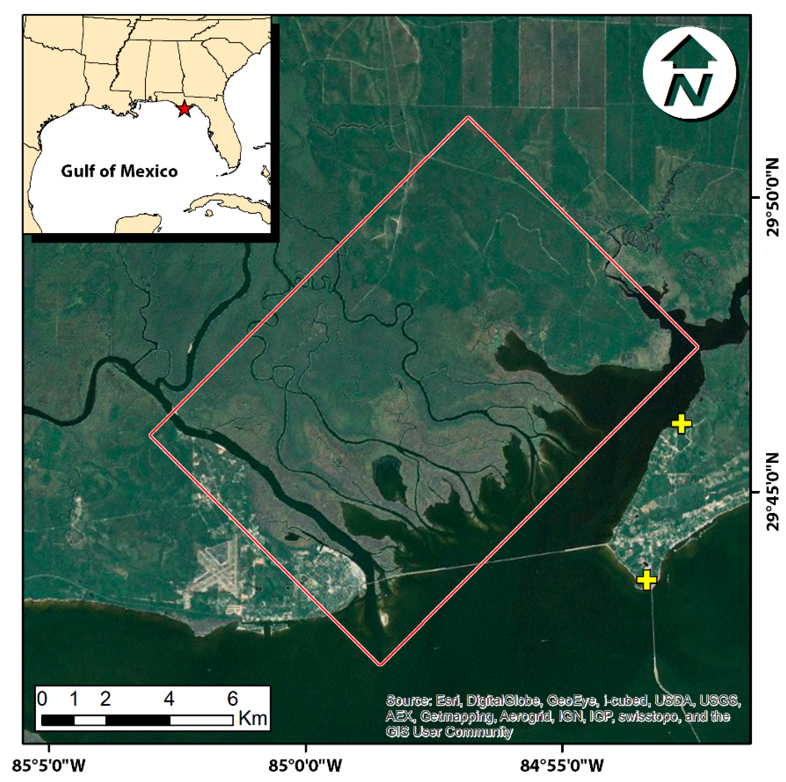
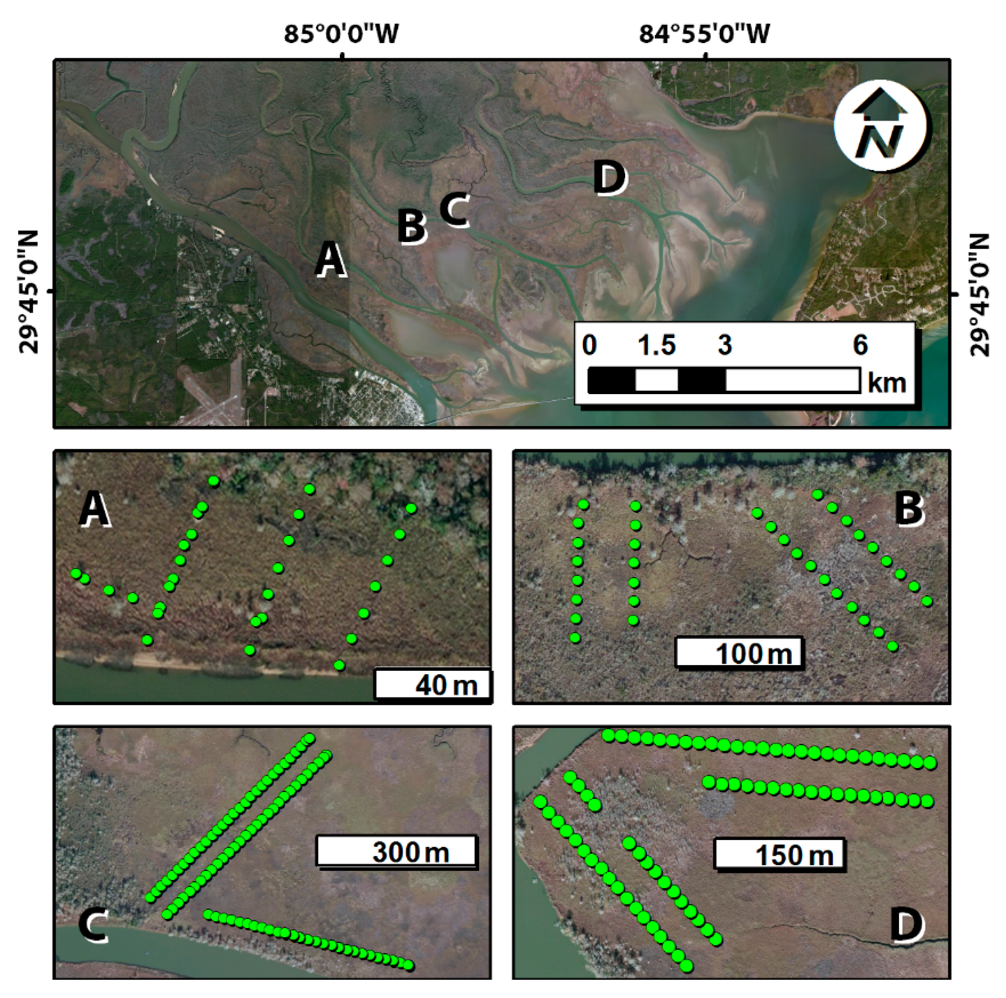
In this study, a combination of field sampling and remote sensing was used to develop linear regression models relating the aboveground biomass density of salt marsh vegetation to variables derived from the remotely sensed data. This study differs from similar work in the past [22] because it is species independent. This paper demonstrates that a combination of optical satellite imagery and data obtained from active remote sensing sources, such as SAR and/or lidar sensors, will explain more of the variation in aboveground biomass than would either data source alone. These species-independent biomass estimates can then be used to classify the aboveground biomass density and develop corresponding lidar DEM correction values.

2. Study Area

This study was conducted at the Apalachicola National Estuarine Research Reserve (ANERR) in the panhandle of northwestern Florida (Figure 1). The ANERR encompasses almost 100,000 ha, including the lower 84 km of the Apalachicola River and its floodplain as well as the entire Apalachicola Bay estuary. The Apalachicola Bay, shielded from the currents of the Gulf of Mexico by a chain of barrier islands, is one of the most productive estuaries in North America. The bay supports a major nursery for commercial fishing and shellfish industries that are worth an estimated $14–16 million in annual revenue; it is also an important foraging area for trans-gulf migratory birds. The ANERR contains an estimated 7864 ha of salt and freshwater marshes [28]. As with other portions of the northwest coast of Florida, ANERR salt marshes are characterized as “low marsh,” consisting of tall seaward fringes of Spartina spp. (cordgrass) and J. roemerianus, and “high marsh,” composed of shorter J. roemerianus, Spartina spp., and salt-tolerant halophytes such as Salicornia spp. (saltwort) [4]. Somewhat unique for Gulf Coast salt marshes, however, is that the dominant cordgrass species is Spartina cynosuroides (big cordgrass), rather than S. alterniflora or Spartina patens (saltmeadow cordgrass).
Figure 1. Study area (box) and biomass sampling locations (crosses). A total of 16 biomass samples were taken at the two sites.
Remotesensing 07 03507 g001

3. Data Collection

3.1. Field Sampling

In June and September of 2011, field samples of salt marsh vegetation were collected to calculate the density of aboveground biomass. Two areas of salt marsh on the east side of Apalachicola Bay were selected and are shown in Figure 1. A set of random points was generated within these salt marsh areas, with the sample points spaced a minimum of 15 m apart to provide spatial independence and ensure that they were located in separate ASTER pixels. A 0.25 m × 0.25 m square constructed of PVC pipe was cast near each sampling point. In harvesting the aboveground biomass, we included all vegetation with roots inside the PVC square. Additional samples were obtained by navigating 4.57 m (15 ft) north and east of each sampling point and repeating the harvesting procedure, resulting in three sub-samples per random point. The sampling locations were located outside the study area, but in settings with similar vegetation characteristics, including species and density (Figure 1). This was done to maintain independence between the data used to train and test the biomass density and lidar error regression models.
In the laboratory, all biomass sub-samples were washed, air dried, and separated by species. The sub-samples were then oven dried at 105 °C until constant mass was achieved. The dry biomass density (in g∙m−2) was then calculated for each sub-sample. Finally, the biomass densities of the three sub-samples were averaged to obtain the mean total aboveground biomass density for each sampling point. The standard deviations for the three biomass density subsamples for each site were aggregated to produce an average standard deviation for the entire data set (Table 1).
In January of 2013, the research team collected GPS survey elevations using Real Time Kinematic (RTK) corrections on a 20 m grid covering the above-referenced salt marsh sampling locations. The topographic elevations were checked at six steel rod benchmarks set by the National Atmospheric and Oceanographic Administration (NOAA), National Geodetic Survey (NGS). The accuracies of these survey points are approximately 2 cm and 4 cm for the horizontal position and the vertical elevation, respectively. These elevations were used to develop a spatially variable lidar error prediction model based on biomass density.

3.2. Remote Sensing Data

For the optical remote sensing data used in this project, Advanced Spaceborne Thermal Emission and Reflection Radiometer (ASTER) Level 1B satellite imagery was acquired from the United States Geological Survey (USGS) EarthExplorer website. The imagery is delivered as “radiance at the sensor” (W∙m−2∙sr−1∙μm−1) converted to digital number (DN) [29]. The ASTER scene used to develop the biomass regression model and apply it to the study area was acquired on 6 May 2011. This scene was chosen because it was relatively cloud free (<10% cloud cover, with no clouds over study area) and close to the time frame of the field biomass sampling.
Raster datasets of Band 2 (visible red) and Band 3 (near-infrared, NIR) of the ASTER imagery were produced at 15 m spatial resolution. Landsat 5 Enhanced Thematic Mapper imagery was also considered for this analysis; however, it was significantly outperformed by ASTER data in our preliminary analyses for this application and is not discussed further. See Abrams et al. [29] for a comparison of ASTER vs. Landsat TM red and NIR bands. The vegetation index (VI = NIR/red) and the normalized difference vegetation index (NDVI = (NIR – Red)/(NIR + Red)) were calculated to derive two new raster images. The VI and NDVI pixel values closest to each biomass sampling point were extracted from each raster.
IfSAR and lidar were the active remote sensors used to acquire data for our analysis. The IfSAR data were acquired through a license with the Digital Coast program of the NOAA Coastal Services Center. NOAA provided these data as a floating-point digital surface model (DSM) raster with an approximate cell size of just over 4 m. The radar pulse of the IfSAR sensor penetrates vegetation to a level dense enough to cause a reflection. Even for dense vegetation such as marsh grasses, this value is below the actual canopy; however, it is near enough to the top of the vegetation to be interpreted as a measure of relative vegetation canopy elevation [30]. To investigate the effect of varying resolution on overall biomass estimation model performance, the IfSAR data were resampled to generate a series of raster surfaces with coarser resolutions of 10, 15, 20, 25, 30, and 35 m via bilinear interpolation.
The lidar data were acquired for Franklin County, Florida, in the summer of 2007 by contractors to the Florida Division of Emergency Management (FDEM) and are available to the public. These are classified, discrete return lidar data with a required nominal pulse spacing of 1.25 m (4 ft), calculated point cloud density of 4.26 pts∙m−2, and a reported consolidated vertical accuracy (CVA, 95th percentile) of 18.6 cm (0.61 ft) across all terrain types. For the purposes of this study, points in classes 7 (Noise) and 9 (Open Water) were omitted, retaining classes 1 (Unclassified) and 2 (Ground) for analysis [31]. From these data we created two raster surfaces with a cell size of 5 m for ground elevation and canopy elevation. To create the ground elevation raster, we selected only those lidar returns representing the minimum height value in each 5 m × 5 m cell. This method is known as “minimum bin-gridding” and has been used to reduce the vertical errors in digital elevation model (DEM) rasters created from lidar data acquired over areas of dense vegetation, such as salt marshes [32]. For the canopy elevation raster, we selected the returns representing the maximum elevation in each 5 m × 5 m cell. Finally, we generated a canopy height raster surface by subtracting the ground elevation raster surface from the canopy elevation raster surface. As with the vegetation raster surfaces derived from the satellite imagery, we extracted the pixel value closest to each biomass sampling location for the IfSAR- and lidar-derived raster surfaces.
To limit the analysis to emergent wetlands, including the salt marshes, a mask consisting of National Land Cover Database (NLCD) class number 95, Emergent Herbaceous Wetland, was generated (Figure 2). This mask was applied to all subsequent spatial data analyses and regression model development. The NLCD 2011 data development was based largely on analysis of Landsat satellite imagery from 2011 [33].
A summary of all remote sensing and field data is shown in Table 1.
Table 1. Summary of data used in analysis.
Data SetResolutionReported Accuracy *Acquisition DateUse in Study
ASTER Radiance (converted to DN)15 m±4%6 May 2011Biomass regression
IfSAR DSM4 m1 m (vertical)2004Biomass regression
Lidar Point Cloud4 pts/m218.6 cm (vertical)2007Biomass regression (canopy height)
Field Biomass Density (Mean = 1738 g/m2)n/a±691 g/m2 (std dev)Jun, Sep 2011Biomass regression
GPS–RTK Elevationn/a4 cm (vertical)Jan 2013Lidar error regression
Lidar DEM1.52 mTested hereinSummer 2007Basis for adjustment
GPS–RTK Elevationn/a4 cm (vertical)Jan, Apr, Jul 2013Biomass-adjusted DEM testing
* For field biomass density we report variation rather than accuracy.
Figure 2. Remote sensing data within the study area. (A) 2011 National Land Cover Dataset class 95, Emergent Herbaceous Wetland; (B) ASTER Band 2 (red) at 15 m spatial resolution (DN); (C) NOAA Coastal IfSAR DSM (meters) resampled to 15 m spatial resolution; (D) 2007 lidar canopy height (meters) derived from minimum/maximum bin gridding of point files.
Remotesensing 07 03507 g002

4. Analysis and Model Development

4.1. Regression Analysis for Biomass Density

A series of ordinary least squares (OLS) linear regression models was created using the statistical software R version 3.0.2 [34]. The laboratory measured aboveground biomass density of the field samples ranged from 730 to 2934 g∙m−2, with a mean value of 1472 g∙m−2 and a standard deviation of 652 g∙m−2. Please note that these values are different from the values reported in Table 1; Table 1 refers to the mean and standard deviations of the sub-samples at each sampling location.
The histogram of the biomass density values was somewhat right-skewed, suggesting a lognormal distribution (Figure 3, left). Transforming the biomass density values by calculating their natural logarithms improved the normality of the distribution (Figure 3, right). The normality of the natural log-transformed data was confirmed by constructing a normal probability plot (Figure 4) and computing the interquartile range over standard deviation ratio, IQR/s. As shown in Figure 4, the normal probability plot produced a straight line and the computed IQR/s was 1.4, both of which indicated sufficient normality.
Consequently, the natural log-transformed biomass density values were used as the dependent variable in all of the linear regressions. Various combinations of data derived from the remote sensing datasets described in the previous section were the independent variables. To select the best model among the numerous models fitted, the Akaike information criterion (AIC) was used, wherein lower AIC values were indicative of better-fitting, more parsimonious models [35]. The adjusted R2 value for each model was also calculated to indicate the amount of variation in log-transformed biomass density explained by the model while taking into account the number of independent variables. To avoid collinearity in models containing multiple independent variables, Pearson’s correlation coefficients between all of the pairwise combinations of variables were calculated. For models containing independent variables with strong correlations, the variance inflation factor (VIF) scores were calculated using the car package in R [36] to explicitly check for collinearity.
Figure 3. Biomass density distributions. (Left) the untransformed and right-skewed distribution; (Right) natural log-transformed and more normal distribution.
Remotesensing 07 03507 g003
Figure 4. Normal probability plot for natural log of biomass density.
Remotesensing 07 03507 g004
All of the linear regressions of the log-transformed biomass density vs. the independent variables derived from the ASTER imagery were statistically significant (Table 2). The ASTER-derived NDVI and VI (not shown) explained less than 40% of the total variation in biomass density. The red band (ASTER band 2) explained the most variation among the single-variable regressions, with an adjusted R2 value of just over 0.52; on the other hand, combining the red and near-infrared (ASTER band 3) bands in a multiple regression model led to a slightly lower adjusted R2 value of 0.51. Including the IfSAR elevation data as an independent variable produced significantly better models for all of the ASTER band combinations. Overall, the best satellite-only model included the red band and IfSAR data and explained almost 72% of the variation in biomass density. Given that the Pearson’s correlation coefficient between the red band and IfSAR height variables was extremely low (r = 0.08), this model was not likely to be affected by multicollinearity [35].
Resampling the IfSAR elevation data to coarser spatial resolution had a positive impact on the biomass regression results. As shown in Table 2, resampling the IfSAR data to a resolution of 15 m improved the fit of the model, as indicated by the adjusted R2 value of almost 0.74. During the model selection process it was discovered that none of the models based on coarser resolutions of the resampled IfSAR data (20 m, 25 m, 30 m, 35 m) explained as much variation as the model based on the 15 m IfSAR data, although the 30 m model came close with an adjusted R2 value of just under 0.73. This was expected, as it was a multiple of the high performing 15 m resolution. The Pearson’s correlation coefficient between the 15 m resampled IfSAR data and the ASTER band 2 data was slightly higher than the correlation with the original-resolution IfSAR data (r = 0.09 vs. r = 0.08), but still far too low for concern about multicollinearity in the regression model. This lack of collinearity was further confirmed by the fact that both variables in this model have variance inflation factor (VIF) scores that are very close to one, well below the threshold value of 10 [36].
The results of the linear regressions involving the lidar-derived independent variables showed further improvement to the regression model. Neither the single-variable model including ground elevation nor the one including canopy elevation was statistically significant, but the one including canopy height was significant and had an adjusted R2 value of 0.18 (Table 2, first row). The multiple regression model including both canopy height and the ASTER band 2 data was also significant and increased the amount of variation explained by the model to almost 50%. As the final two rows of Table 2 indicate, adding the IfSAR elevation data as an independent variable to the model containing canopy height and ASTER band 2 increased the adjusted R2 value to 0.77 and 0.82 for the original-resolution and 15 m-resampled IfSAR data, respectively. While the correlation between the lidar-derived canopy height and ASTER band 2 variables was fairly strong (r = 0.67), the VIF scores do not indicate any strong collinearity in the model, since the highest score was VIF = 2.41 for canopy height.
Table 2. Biomass density vs. ASTER and IfSAR.
Independent Variable(s)P-ValueAdjusted R2AIC
Canopy Height0.03780.184627.9963
Canopy Height + Aster_Band20.00170.492719.8279
Aster_Band2 (red)0.00030.521917.8547
Aster_Band2 + IfSAR<0.00010.71608.8048
Aster_Band2 + IfSAR_15m<0.00010.73917.1929
Canopy Height + Aster_Band2 + IfSAR<0.00010.76955.6162
Canopy Height + Aster_Band2 + IfSAR_15m<0.00010.82470.4117
This regression model was accepted for the computation of log-transformed biomass density. The regression model coefficients are shown in Table 3.
Table 3. Biomass density estimation regression model coefficients.
Independent VariableCoefficient
Intercept6.5430
Canopy Height−1.6838
Aster_Band20.0196
IfSAR_15m0.8703

4.2. Regression Analysis for Lidar Error

The log-transformed biomass was used as the lone independent variable in the regression to calculate lidar error. Recall that lidar error is defined as the difference between the “true” elevation as determined by GPS-RTK surveying and the lidar DEM. To more accurately model the physical relation between biomass and lidar error, it is assumed that an area with zero biomass density represents a perfectly flat and unobstructed surface. In turn, it is assumed that an area with zero biomass will not contribute any obstruction error, i.e., false ground classifications due to laser returns from vegetation. Therefore, the regression between lidar error and log-transformed biomass will be forced through the origin (having an intercept value of zero). The regression achieved an adjusted R2 of 0.829 and was statistically significant with a p value less than 0.001. Note that since this was a linear regression with only one independent variable, the AIC and VIF measures were unnecessary. This regression model was accepted for the computation of log-transformed biomass density. The regression model coefficients are shown in Table 4.
To test the accuracy of the adjusted lidar DEM, 229 spot elevations within the Emergent Herbacaeous Wetland landcover class were obtained during a transect-based GPS-RTK survey in the lower Apalachicola River marsh (Figure 5). Transects were deliberately oriented on varying directional headings and the sites were selected to span the fluvial distributary network within the study area.
Figure 5. Spot elevations for testing accuracy of biomass-adjusted DEM.
Remotesensing 07 03507 g005
Table 4. Regression coefficients for estimation of lidar error.
Independent VariableCoefficient
Intercept0.0000
LN_BiomassDensity0.0323

4.3. Categorization of Biomass Estimates

Although the data shown in Section 4.1 and Section 4.2 seem to support the estimation of numerical values for the biomass density and lidar error, the sample size was small and, as a result, we cannot state with certainty that a value of biomass density represented the true conditions on the ground. However, using the field samples, we could classify the biomass density values as high, medium, or low. This enables relative comparisons of biomass distribution over time in studies focusing on the effects of sea level rise, for example. Table 5 shows the field samples along with their respective lidar DEM errors.
Table 5. Classification of biomass (BM) density relative to lidar error.
BM (g/m2)Ln(BM)RankPercentileLidar DEM Error (m)
29347.98421100.00%0.30
26417.8790293.30%0.18
18857.5417386.60%0.35
18077.4994480.00%0.21
18027.4968573.30%0.27
17627.4739666.60%0.09
16997.4377760.00%0.26
15447.3423853.30%0.10
15327.3343946.60%0.35
9496.85501040.00%0.34
9166.82051133.30%0.15
8926.79391226.60%0.29
8256.71521313.30%0.17
8256.71521313.30%0.26
8046.6899156.60%0.20
7306.5931160.00%0.22
We pursued two scenarios for adjusting the lidar DEM based on estimated biomass density: a division into three classes (High, Medium, and Low), where the thresholds were at the approximate 66th and 33rd percentile values of biomass density (1800 g∙m−2 and 950 g∙m−2, respectively), and a division into two classes (High and Low), with a single threshold value at the natural break occurring at the approximate 45th percentile (1500 g∙m−2). These adjustment scenarios were compared against the overall median value lidar DEM error for the entire set of samples. Refer to Table 6 below for adjustment values.
These classifications of the field samples formed the basis of the lidar DEM error adjustment values. The adjustments were used to modify (lower) the lidar DEM to more accurately reflect the true in situ conditions. To capture some of the non-linearity in the lidar error as a function of biomass density, a quartile-based approach was used within each class. We selected the upper quartile (75th percentile) lidar DEM error as the adjustment value for lidar DEM errors associated with the High biomass density class, the median (50th percentile) value for the Medium class, and the lower quartile (25th percentile) for the Low class. This approach was pursued to investigate whether lidar DEM error due to vegetation was disproportionately greater in areas of high density and effectively non-existent in areas with sparse vegetation. The presence of biomass always results in a lidar DEM elevation that is too high; therefore, all adjustments we made were applied to lower the lidar DEM elevation (Table 6).
The three- and two-class estimation schemes of biomass density we used to adjust the lidar DEM with the quartile and median selection methods resulted in four adjustment scenarios. A single biomass density class with a median adjustment value (termed the “control” scenario) is presented for comparison. For all scenarios, the adjustment value was subtracted from the lidar DEM elevation value in each pixel based on the biomass density class. Two z-tests (α = 0.05) were performed: first, the mean error of the adjustment scenarios was compared with the mean error of the lidar DEM; second, the mean error of the adjustment scenarios was compared with the mean error of the control scenario.
Table 6. Lidar corrections based on biomass density class.
Biomass Density3-Class, Quartile Adjustment (m)3-Class, Median Adjustment (m)2-Class, Quartile Adjustment (m)2-Class, Median Adjustment (m)1-Class, Median Adjustment (m)
High0.320.270.300.26
Medium0.230.26 0.24
Low0.160.210.180.22

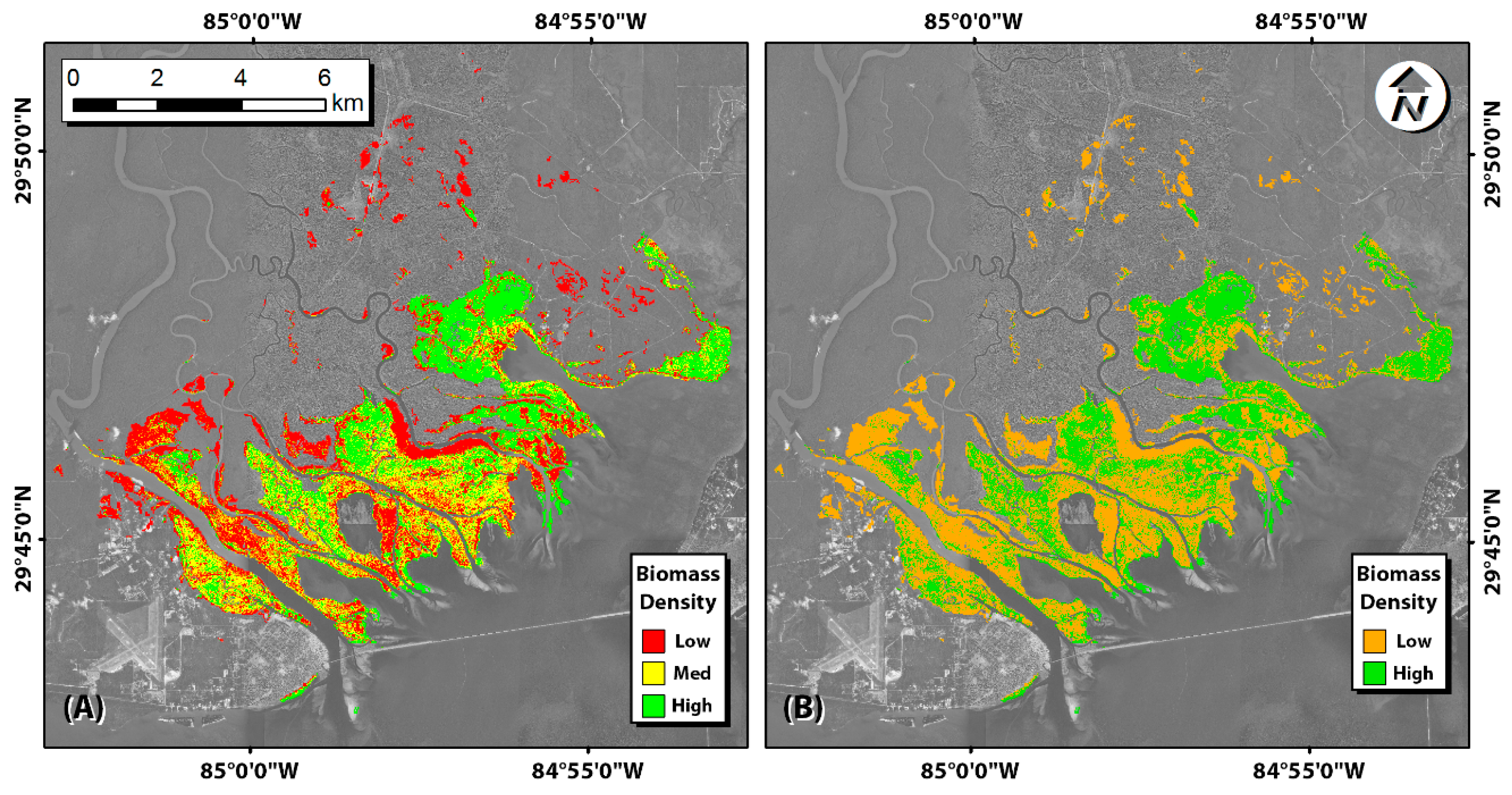
5. Results and Discussion

Using this newly developed regression model, spatially variable biomass densities were estimated for the study area (Figure 6).
Figure 6. Biomass density classifications for study area. (A) Three-class scheme: High, Medium, and Low; (B) Two-class scheme: High and Low.
Remotesensing 07 03507 g006
The results of the first comparison overwhelmingly showed that the mean errors for all adjustment scenarios, including the control, were significantly less than the lidar DEM (therefore, we do not show those results here in detail). The errors between the DEM for each scenario and the GPS-RTK measured elevation at the 229 testing points, including the p value for the second z-test, are shown in Table 7.
Table 7. Errors in the lidar and biomass-adjusted DEMs. The p value represents the probability that the mean error of the control (single-class median) scenario is greater than the mean error for a particular adjustment scenario.
MeasureLidar DEM (m)3-Class, Quartile Adjustment (m)3-Class, Median Adjustment (m)2-Class, Quartile Adjustment (m)2-Class, Median Adjustment (m)1-Class, Median Adjustment (m)
RMSE0.650.420.420.400.420.44
Mean Error0.610.340.340.320.350.37
Std. Dev. Error0.240.250.240.240.240.24
p value1.0000.0500.0600.0010.134n/a
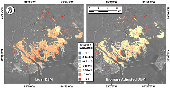
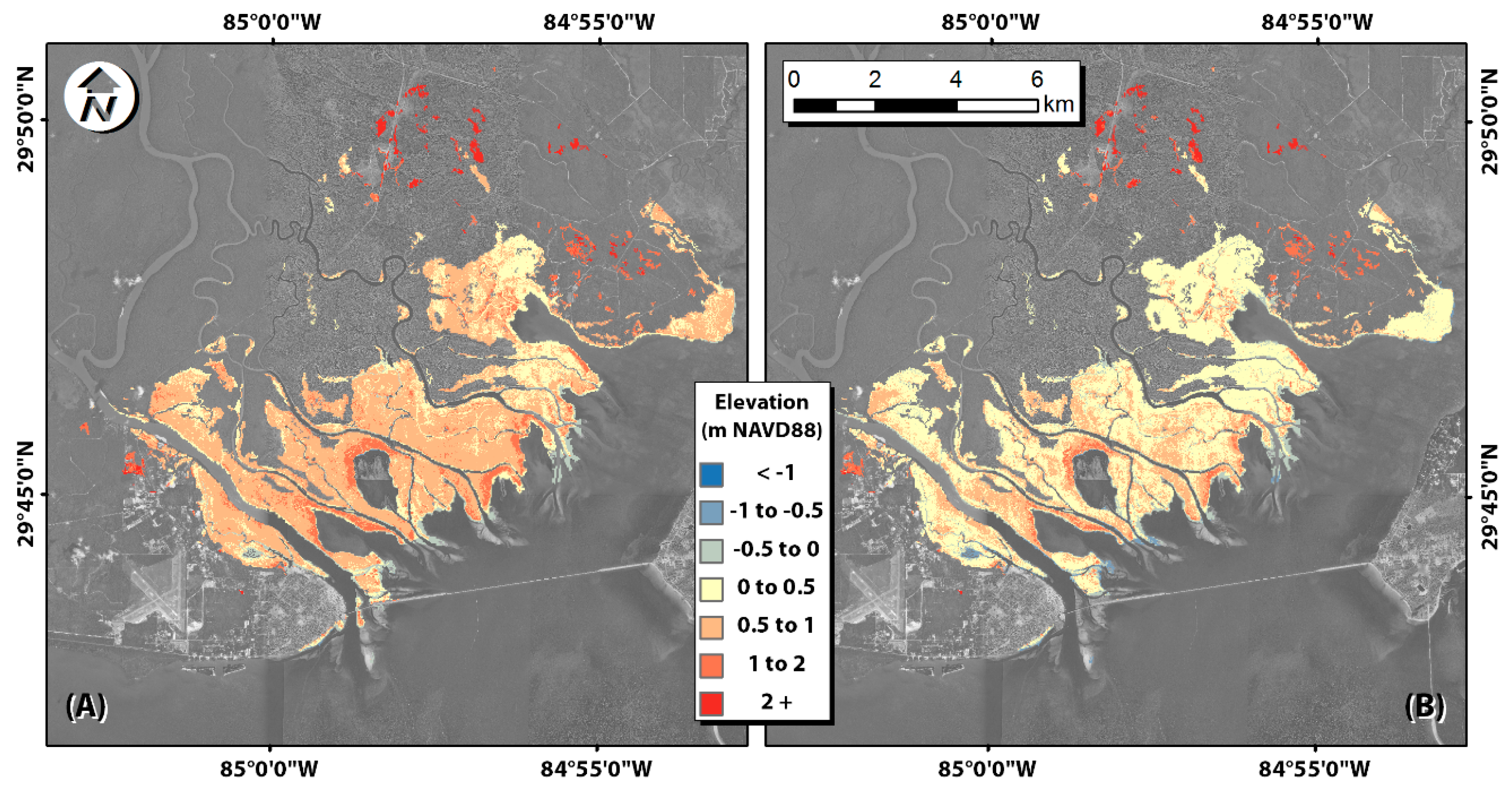
As shown, the biomass-adjusted DEMs resulted in an average reduction in the Root Mean Square (RMS) error from 0.65 m to 0.42 m, representing a 35% decrease. All adjustment scenarios performed better than simply using the overall median adjustment across the entire DEM; however, only the quartile-based adjustments were statistically significant. Also, the two-class scheme performed slightly better than the three-class scheme, indicating that detecting natural breaks in the biomass density sample population was a better approach than arbitrarily splitting it into three classes with an approximately equal number of samples. The best performing adjustment scenario was the two-class quartile scenario. This was likely due to the better performance of the two-class scheme and the better capture of the non-linear nature of the lidar error/biomass density relationship. For comparison, the lidar DEM and the two-class, quartile-adjusted DEM are shown in Figure 7.
Figure 7. (A) Lidar DEM and (B) two-class, quartile-adjusted DEM.
Remotesensing 07 03507 g007
The adjusted DEM contained many more pixels in the 0–0.5 m range than did the original lidar DEM (Figure 7), which is the expected range for the marsh platform. The marsh platform typically is slightly higher than mean sea level, and the marsh is the most productive when an optimal periodic inundation occurs. In this region, mean sea level and mean high water are approximately 4.5 and 22.8 cm above NAVD88, respectively.
These findings must be tempered by the fact that even with the technique proposed here, the error is still more than we would like, especially in microtidal systems such as the northern Gulf of Mexico. In contrast, results achieved by Hladik and Alber [22] showed a reduction in mean DEM error from 0.10 m to −0.01 m using a species and vegetation-height specific adjustment methodology. Notably, that study site (Sapelo Island, Georgia) had substantially less error between the lidar DEM and GPS-RTK elevations than did Apalachicola (0.10 vs. 0.61 m), so a direct comparison with the results presented here is difficult. However, if one is able to generate or obtain spatially distributed species classification along with vegetation height classes, the method of Hladik and Alber is likely superior. If these data are not available, we recommend the method proposed here. In any case, we would caution against blindly using this or any other method without first verifying that it is applicable in the tidal, vegetation type and density conditions of a particular study site. This can be accomplished by conducting an exploratory field data acquisition and remote sensing analysis campaign, using the method presented here as guidance.
To view these findings in their proper context, assessments of the processing sequence and potential sources of error are required. First, the lidar elevation accuracy standard set by the US Federal Emergency Management Agency is 36.6 cm (1.19 ft) at the 95% confidence level, so most lidar surveys in coastal areas are designed to meet this standard. Oftentimes the vertical elevation accuracy in open terrain is closer to 15 cm [37]. The lidar data used in this study met that standard, but for microtidal systems, even acceptable lidar accuracy may not be enough for some coastal modeling applications (one of the primary uses of lidar DEMs).
Another potential source of error is the acquisition time of the remote sensing data, especially with respect to the seasonality of the marsh vegetation growth cycle. Depending on the time of year, the marsh grasses may be at their peak or dormant heights. For this study, the field biomass density samples and the ASTER imagery were collected in comparable years (June/September 2011 and May 2011), but there was a seasonal discrepancy. With optical-IR sensors, such as ASTER, it is more difficult to obtain cloud-free imagery in Florida during the summer growing season due to the general storminess of that time period.
The acquisition times of the elevation data (IfSAR DSM, lidar, and GPS-RTK) were substantially disparate (2004, 2007, and 2013, respectively). This is not unusual, as IfSAR and lidar data are expensive and are not collected on a regular basis in most areas. With respect to the difference between the lidar elevations and the GPS-RTK elevations, their separation in time could have been influenced by accretion or erosion in the marsh. Although it is true that there is likely to have been accretion on the marsh surface, it has been estimated to be about 0.8 mm∙yr-1 in Apalachicola [38]. This would have resulted in an accretion of approximately 5 mm, well within the accuracy bounds of the lidar, so is unlikely to have contributed significantly to the error in the regression model. However, the IfSAR data were much older and the month of acquisition could not be determined from the metadata. As the IfSAR provided a measure of canopy elevation, rather than a relative measure such as canopy height, this may have impacted the results significantly.
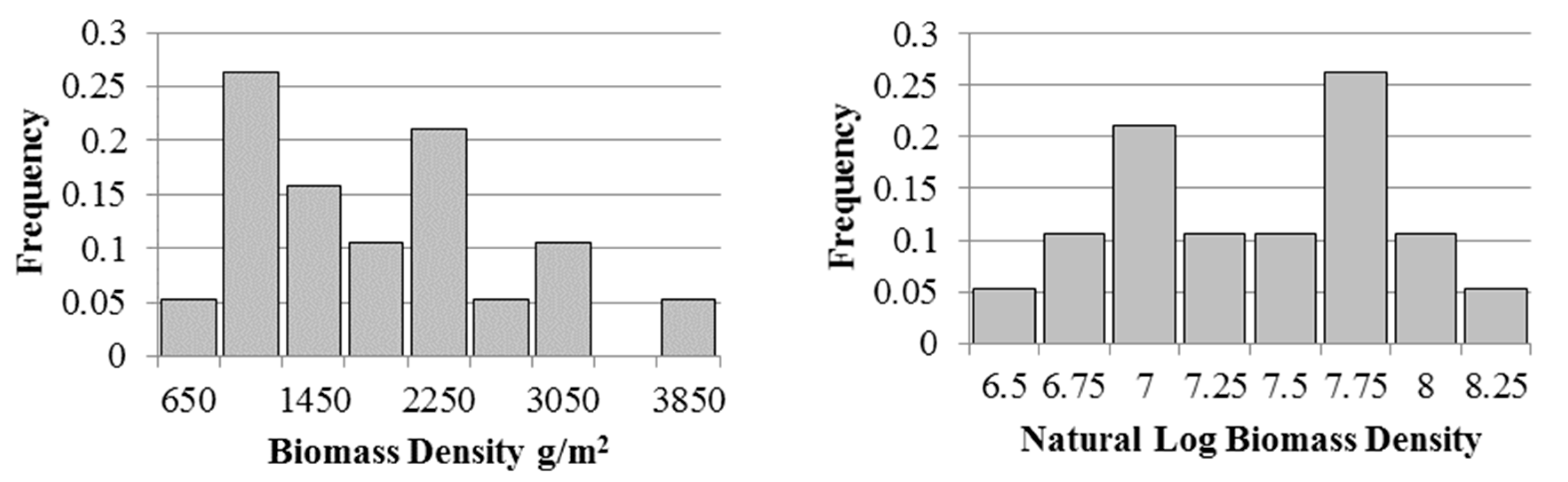
Lastly, the relatively small sample size for field-harvested biomass density (n = 16) requires further caution when applying the technique proposed herein. When using this technique in areas containing comparatively more or less dense marsh vegetation, additional samples should be acquired to adapt the technique for those areas.
Future studies are advised to obtain larger biomass density sample sizes and synchronize the field data collection with the remote sensing and lidar acquisition times to the maximum extent possible. At a minimum, data should be synchronized on a seasonal basis. Furthermore, biomass growth rates can vary year to year due to climatic, weather, and environmental factors such as drought, severe storms, or a pollution event. Any evidence of abnormal growth patterns should be addressed.
Despite the uncertainty in the method proposed herein, it is still a substantial step in the right direction and a necessary attempt to address a problem with widespread implications. The elevation of the marsh platform is a key parameter in nearly every model set in coastal ecosystems. For example, the Marsh Equilibrium Model [24] relies heavily on the initial estimation of the marsh platform elevation to project future accretion in response to sea level rise. The model is based on local bioassay field experiments that estimate above- and below-ground biomass production rates that also serve as inputs into the model.
The Sea Level Affecting Marshes Model (SLAMM) [39] is another widely used tool that relies heavily on marsh platform elevation as an input. The technical documentation for this model specifically states that bare earth lidar should be used as the elevation dataset when available [40]. If the mean elevation error in a bare earth lidar DEM is nearly 50 cm above its true elevation, regions with small tide ranges such as the northern Gulf of Mexico will not see any modeled inundation, as the erroneously high marsh platform often will exceed the elevation of high tide. With a tool as widely used as SLAMM, this could lead to the propagation of misinformation, with communities basing their future land planning decisions on highly inaccurate results. In fact, Freeman et al. [38] applied the SLAMM model to Apalachicola Bay in 2012 and used the same lidar DEM that served as the basis for adjustment in this paper (1.524 m (5 ft) resolution resampled to 30 m). Their results serve as guidance for adapting to projected impacts to coastal wetlands, infrastructure, and vulnerable species, thereby demonstrating the importance of addressing the issue of inaccuracies in lidar DEMs of coastal salt marshes.

6. Summary and Conclusions

A novel processing sequence that uses ASTER, IfSAR, and lidar data to estimate spatially variable biomass density classes is presented. Two biomass density classification schemes were tested: a three-class scheme (high, medium, and low) based on the 66th and 33rd percentiles, and a two-class scheme (high and low) based on a natural break at the 45th percentile in the field biomass density data. These biomass density classes were used to estimate the error in the lidar DEM of the marsh platform. To compute the lidar DEM adjustment value, the field biomass samples (n = 16) and their corresponding lidar DEM errors were analyzed. Within each classification scheme, two methods for computing the recommended adjustment values were investigated: a median approach, where the 50th percentile lidar DEM error within each class was selected, and a quartile approach, where the 75th percentile lidar DEM error within the high class, the 50th percentile within the medium class, and the 25th percentile with the low class were selected. All combinations of biomass density classification scheme and adjustment value were tested. All adjustment schemes were superior to the unadjusted lidar DEM by wide statistical margins. The schemes were also compared to a simple median adjustment based on the entire population of samples. Only the scenarios using the quartile adjustment selection were significantly better than simply using the overall median lidar DEM error. The two-class quartile adjustment method was most effective. The recommended adjustments associated with each of these classes are 0.30 m for high and 0.18 m for low. The performance of the method was tested on 229 spot elevation points in the lower Apalachicola River Marsh. The two-class quartile-adjusted DEM reduced the RMS error in elevation from 0.65 m to 0.40 m, a 38% improvement. The raw mean errors for the lidar DEM and the adjusted DEM were 0.61 ± 0.24 m and 0.32 ± 0.24 m, respectively, thereby reducing the high bias by approximately 49%.
Based on the findings of this study and the work by others cited herein, coastal researchers should avoid using unadjusted lidar DEMs in coastal marshes and wetlands dominated by emergent vegetation. Instead, they are advised to apply a spatially variable correction technique such as the one presented here. Future work in developing these techniques should address the major sources of uncertainty identified in this paper, namely the discrepancy in acquisition time between field and remote sensing datasets.

Acknowledgments

This study is funded in part under U.S. National Oceanic and Atmospheric Administration (NOAA) Grant NA10NOS4780146 and the Louisiana Sea Grant Laborde Chair endowment. The statements, findings, conclusions, and recommendations expressed herein are those of the authors and do not necessarily reflect the views of NOAA. The authors would also like to acknowledge the guest editor of this special issue as well as the reviewers for their suggestions to improve this paper.

Author Contributions

All authors contributed to the scientific content and authorship of this paper.

Conflicts of Interest

The authors declare no conflict of interest.

References

  1. Kennish, M.J. Coastal salt marsh systems in the US: A review of anthropogenic impacts. J. Coast. Res. 2001, 17, 731–748. [Google Scholar]
  2. Barbier, E.B.; Hacker, S.D.; Kennedy, C.; Koch, E.W.; Stier, A.C.; Silliman, B.R. The value of estuarine and coastal ecosystem services. Ecol. Monogr. 2011, 81, 169–193. [Google Scholar] [CrossRef]
  3. Jensen, J.R.; Olson, S.R.; Schill, S.R.; Porter, D.E.; Morris, J.T. Remote sensing of biomass, leaf-area-index, and chlorophyll a and b content in the ACE Basin National Estuarine Research Reserve using sub-meter digital camera imagery. Geocarto Int. 2002, 17, 27–36. [Google Scholar] [CrossRef]
  4. Mitsch, W.J.; Gosselink, J.G. Wetlands; John Wiley & Sons, Inc.: New York, NY, USA, 2000. [Google Scholar]
  5. Gedan, K.B.; Silliman, B.R.; Bertness, M.D. Centuries of human-driven change in salt marsh ecosystems. Annu. Rev. Mar. Sci. 2009, 1, 117–141. [Google Scholar] [CrossRef]
  6. Silliman, B.R.; Grosholz, T.; Bertness, M.D. Salt marshes under global siege. In Human Impacts on Salt Marshes: A Global Perspective; Silliman, B.R., Grosholz, T., Bertness, M.D., Eds.; University of California Press: Berkeley, CA, USA, 2009; pp. 391–398. [Google Scholar]
  7. Vermeer, M.; Rahmstorf, S. Global sea level linked to global temperature. Proc. Natl. Acad. Sci. USA 2009, 106, 21527–21532. [Google Scholar] [CrossRef] [PubMed]
  8. Nicholls, R.J.; Cazenave, A. Sea-level rise and its impact on coastal zones. Science 2010, 328, 1517–1520. [Google Scholar] [CrossRef] [PubMed]
  9. Intergovernmental Panel on Climate Change. Climate Change 2014: Impacts, Adaptation, and Vulnerability. Part A: Global and Sectoral Aspects. Contribution of Working Group II to the Fifth Assessment Report of the Intergovernmental Panel on Climate Change; Field, C.B., Barros, V.R., Dokken, D.J., Mach, K.J., Mastrandrea, M.D., Bilir, T.E., Chatterjee, M., Ebi, K.L., Estrada, Y.O., Genova, R.C., et al., Eds.; Cambridge University Press: Cambridge, UK and New York, NY, USA, 2014; p. 1132. [Google Scholar]
  10. Parris, A.; Bromirski, P.; Burkett, V.; Cayan, D.; Culver, M.; Hall, J.; Horton, R.; Knuuti, K.; Moss, R.; Obeysekera, J.; et al. Global Sea Level Rise Scenarios for the US National Climate Assessment; NOAA Tech Memo OAR CPO-1: Washington, DC, USA, 2012; p. 37. [Google Scholar]
  11. Orson, R.; Panageotou, W.; Leatherman, S.P. Response of tidal salt marshes of the US Atlantic and Gulf coasts to rising sea levels. J. Coast. Res. 1985, 1, 29–37. [Google Scholar]
  12. Hardisky, M.A.; Gross, M.A.; Klemas, V. Remote sensing of coastal wetlands. BioScience 1986, 36, 453–460. [Google Scholar] [CrossRef]
  13. Zhang, M.; Ustin, S.L.; Rejmankova, E.; Sanderson, E.W. Monitoring Pacific coast salt marshes using remote sensing. Ecol. Appl. 1997, 7, 1039–1053. [Google Scholar] [CrossRef]
  14. Waring, R.H.; Way, J.; Hunt, E.R.; Morrissey, L.; Ranson, K.J.; Weishampel, J.F.; Oren, R.; Franklin, S.E. Imaging radar for ecosystem studies. BioScience 1995, 45, 715–723. [Google Scholar] [CrossRef]
  15. Lu, D. The potential and challenge of remote sensing-based biomass estimation. Int. J. Remote Sens. 2006, 27, 1297–1328. [Google Scholar] [CrossRef]
  16. Andersen, H.E.; Reutebuch, S.E.; McGaughey, R.J. Active remote sensing. In Computer Applications in Sustainable Forest Management: Including Perspectives on Collaboration and Integration; Shao, G., Reynolds, K.M., Eds.; Springer: Dordrecht, The Netherlands, 2006; pp. 43–66. [Google Scholar]
  17. Moghaddam, M.; Dungan, J.L.; Acker, S. Forest variable estimation from fusion of SAR and multispectral optical data. IEEE Trans. Geosci. Remote Sens. 2002, 40, 2176–2187. [Google Scholar] [CrossRef]
  18. Chen, W.; Blain, D.; Li, J.; Keohler, K.; Fraser, R.; Zhang, Y.; Leblanc, S.; Olthof, I.; Wang, J.; McGovern, M. Biomass measurements and relationships with Landsat 7 ETM+ and JERS 1 SAR data over Canada’s western sub-arctic and low arctic. Int. J. Remote Sens. 2009, 30, 2355–2376. [Google Scholar] [CrossRef]
  19. Balzter, H. Forest mapping and monitoring with interferometric synthetic aperture radar (InSAR). Prog. Phys. Geogr. 2001, 25, 159–177. [Google Scholar] [CrossRef]
  20. Chen, Q.; Laurin, G.V.; Battles, J.J.; Saah, D. Integration of airborne lidar and vegetation types derived from aerial photography for mapping aboveground live biomass. Remote Sens. Environ. 2012, 121, 108–117. [Google Scholar] [CrossRef]
  21. Bilskie, M.V.; Hagen, S.C. Topographic Accuracy Assessment of Bare Earth lidar-derived Unstructured Meshes. Adv. Water Resour. 2013, 52, 165–177. [Google Scholar] [CrossRef]
  22. Hladik, C.; Alber, M. Accuracy assessment and correction of a LIDAR-derived salt marsh digital elevation model. Remote Sens. Environ. 2012, 121, 224–235. [Google Scholar] [CrossRef]
  23. Chen, C.; Qi, J.; Li, C.; Beardsley, R.C.; Lin, H.; Walker, R.; Gates, K. Complexity of the flooding/drying process in an estuarine tidal-creek salt-marsh system: An application of FVCOM. J. Geophys. Res. 2008, 113, 1–21. [Google Scholar]
  24. Morris, J.T.; Sundareshwar, P.V.; Nietch, C.T.; Kjerfve, B.; Cahoon, D.R. Responses of coastal wetlands to rising sea level. Ecology 2002, 83, 2869–2877. [Google Scholar] [CrossRef]
  25. Hagen, S.C.; Morris, J.T.; Bacopoulos, P.; Weishampel, J.F. Sea-level rise impact on a salt marsh system of the lower St. Johns River. J. Waterw. Harb. Coast. Eng. Div. 2013, 139, 118–125. [Google Scholar] [CrossRef]
  26. Passeri, D.L.; Hagen, S.C.; Bilskie, M.V.; Medeiros, S.C. On the significance of incorporating shoreline changes for evaluating coastal hydrodynamics under sea level rise scenarios. Nat. Hazards 2015, 75, 1599–1617. [Google Scholar] [CrossRef]
  27. Bilskie, M.V.; Hagen, S.C.; Medeiros, S.C.; Passeri, D.L. Dynamics of sea level rise and coastal flooding on a changing landscape. Geophys. Res. Lett. 2014, 41, 927–934. [Google Scholar] [CrossRef]
  28. Edmiston, H.L. A River Meets the Bay: the Apalachicola Estuarine System; Apalachicola National Estuarine Research Reserve, Florida Department of Environmental Protection: Apalachicola, FL, USA, 2008. [Google Scholar]
  29. Abrams, M.; Hook, S.; Ramachandran, B. ASTER User Handbook, v2: Advanced Spaceborne Thermal Emission and Reflection Radiometer; National Aeronautics and Space Administration Jet Propulsion Laboratory: Pasadena, CA, USA, 2002. [Google Scholar]
  30. Schmid, K.B.; Hadley, B.; Carter, J. Evaluation of ADS40 and IfSAR Derived High-Spatial Resolution Topographic Data Products for Coastal Resource Management Applications; National Oceanic and Atmospheric Administration: Washington, DC, USA, 2007. [Google Scholar]
  31. Dewberry. Final Report of Specific Purpose Lidar Survey—Lidar, Breaklines and Contours for Franklin County Florida; Florida Division of Emergency Management: Tallahassee, FL, USA, 2009; p. 248. [Google Scholar]
  32. Schmid, K.B.; Hadley, B.; Wijekoon, N. Vertical accuracy and use of topographic LIDAR data in coastal marshes. J. Coast. Res. 2011, 27, 116–132. [Google Scholar] [CrossRef]
  33. Jin, S.; Yang, L.; Danielson, P.; Homer, C.; Fry, J.; Xian, G. A comprehensive change detection method for updating the National Land Cover Database to 2011. Remote Sen. Environ. 2013, 132, 159–175. [Google Scholar] [CrossRef]
  34. R Development Core Team. R: A Language and Environment for Statistical Computing; R Development Core Team: Vienna, Austria, 2011. [Google Scholar]
  35. Quinn, G.P.; Keough, M.J. Experimental Design and Data Analysis for Biologists; Cambridge University Press: Cambridge, UK, 2002. [Google Scholar]
  36. Fox, J.; Weisberg, S. An R companion to applied regression, 2nd ed.; SAGE Publications, Inc.: Thousand Oaks, CA, USA, 2010. [Google Scholar]
  37. Maune, D.F. Digital Elevation Model Technologies and Applications: The DEM Users Manual, 2nd ed.; American Society for Photogrammetry and Remote Sensing: Bethesda, MD, USA, 2007. [Google Scholar]
  38. Freeman, K.; Geselbracht, L.; Gordon, D.; Kelly, E.; Racevskis, L. Understanding Future Sea Level Rise Impacts on Coastal Wetlands in the Apalachicola Bay Region of Florida’s Gulf Coast; Florida Department of Environmental Protection: Tallahassee, FL, USA, 2012; p. 60. [Google Scholar]
  39. Park, R.A.; Trehan, M.S.; Mausel, P.W.; Howe, R.C. The effects of sea level rise on US coastal wetlands. The Potential Effects of Global Climate Change in the United States; Smith, J.B., Tirpak, D.A., Eds.; US Environmental Protection Agency: Washington, DC, USA, 1989. Available online: http://research.fit.edu/sealevelriselibrary/documents/doc_mgr/452/US_Effects_of_SLR_on_Coastal_Wetlands_-_Park_et_al._1989.pdf (accessed on 25 March 2015).
  40. SLAMM 6.2 Technical Documentation; Warren Pinnacle Consulting, Inc.: Waitsfield, VT, USA, 2012.

