Self-Adaptive Gradient-Based Thresholding Method for Coal Fire Detection Using ASTER Thermal Infrared Data, Part I: Methodology and Decadal Change Detection

Du, Xiaomin; Cao, Daiyong; Mishra, Deepak; Bernardes, Sergio; Jordan, Thomas R.; Madden, Marguerite

doi:10.3390/rs70606576

Open AccessArticle

Self-Adaptive Gradient-Based Thresholding Method for Coal Fire Detection Using ASTER Thermal Infrared Data, Part I: Methodology and Decadal Change Detection

¹

School of Geosciences and Surveying Engineering, China University of Mining & Technology, Beijing 100083, China

²

Center for Geospatial Research, Department of Geography, The University of Georgia, Athens, GA 30602, USA

³

Biospheric Sciences Laboratory, The National Aeronautics and Space Administration (NASA) Goddard Space Flight Center, Greenbelt, MD 20771, USA

^*

Author to whom correspondence should be addressed.

Remote Sens. 2015, 7(6), 6576-6610; https://doi.org/10.3390/rs70606576

Submission received: 8 October 2014 / Revised: 22 April 2015 / Accepted: 18 May 2015 / Published: 26 May 2015

(This article belongs to the Special Issue Recent Advances in Thermal Infrared Remote Sensing)

Download

Browse Figures

Versions Notes

Abstract

:

Coal fires that are induced by natural spontaneous combustion or result from human activities occurring on the surface and in underground coal seams destroy coal resources and cause serious environmental degradation. Thermal infrared image data, which directly measure surface temperature, can be an important tool to map coal fires over large areas. As the first of two parts introducing our coal fire detection method, this paper proposes a self-adaptive threshold-based approach for coal fire detection using ASTER thermal infrared data: the self-adaptive gradient-based thresholding method (SAGBT). This method is based on an assumption that the attenuation of temperature along the coal fire’s boundaries generates considerable numbers of spots with extremely high gradient values. The SAGBT method applied mathematical morphology thinning to skeletonize the potential high gradient buffers into the extremely high gradient lines, which provides a self-adaptive mechanism to generate thresholds according to the thermal spatial patterns of the images. The final threshold was defined as an average temperature value reading from the high temperature buffers (segmented by 1.0 σ from the mean) and along a sequence of extremely high gradient lines (thinned from the potential high gradient buffers and segmented within the lower bounds, ranging from 0.5 σ to 1.5 σ and with an upper bound of 3.2 σ, where σ is the standard deviation), marking the coal fire areas. The SAGBT method used the basic outer boundary of the coal-bearing strata to simply exclude false alarms. The intermediate thresholds reduced the coupling with the temperature and converged by changing the potential high gradient buffers. This simple approach can be economical and accurate in identifying coal fire areas. In addition, it allows for the identification of thresholds using multiple ASTER TIR scenes in a consistent and uniform manner, and supports long-term coal fire change analyses using historical images in local areas. This paper focuses on the introduction of the methodology. Furthermore, an improvement to SAGBT is proposed. In a subsequent paper, subtitled “Part 2, Validation and Sensitivity Analysis,” we address satellite-field simultaneous observations and report comparisons between the retrieved thermal anomalies and field measurements in different aspects to prove that the coal fires are separable by the SAGBT method. These comparisons allowed us to estimate the accuracy and biases of the SAGBT method. As an application of the SAGBT, a relationship between coal fires’ decadal variation and coal production was also examined. Our work documented a total area increase in the beginning of 2003, which correlates with increased mining activities and the rapid increase of energy consumption in China during the decade (2001–2011). Additionally, a decrease in the total coal fire area is consistent with the nationally sponsored fire suppression efforts during 2007–2008. It demonstrated the applicability of SAGBT method for long-term change detection with multi-temporal images.

Keywords:

spontaneous coal combustion; gradient convolution; mathematical morphology thinning; gradient thresholding method; temperature and emissivity separated (TES) algorithm; long-term monitoring

Graphical Abstract

1. Introduction

Coal fires, which occur on the surface (primarily in coal waste piles) and in underground coal seams and are caused by spontaneous combustion, natural events (lightning, forest fires, and peat fires), and human activities (mining and domestic fires), cause severe environmental effects. These effects include noxious gas emissions (e.g., SO₂, NO, CO, and CH₄), an increased concentration of heavy metals in the soil (e.g., mercury, zinc, copper, lead, iron, and germanium), and land surface effects associated with fissures, cracks, land subsidence, and collapse [1,2,3,4,5,6]. Coal fires can also be responsible for the total or partial loss of the coal resource. According to the literature [7], the annual CO₂ emission of the Wuda syncline amounts to 90,000 to 360,000 tons.

The methods involved in the detection of coal fires typically incorporate the identification of changes in the land surface temperature, electrical conductivity, magnetic field, heavy metal concentration, and gas emissions, whereas remote sensing-based coal fire research mainly focuses on coal fire-related thermal anomaly detection [8]. The first reported study on the detection of spontaneous coal seam combustion and used infrared photography in coal waste pile fires [9]. Through developments in airborne thermal infrared sensors, coal fires and the depth of burning were detected in Pennsylvania [10]. Airborne thermal infrared data acquired during the daytime and nighttime have been used to identify high-temperature targets against low-temperature backgrounds [11]. Then, the use of orbital images (Landsat-5 Thematic Mapper (TM) and NOAA-9 AVHRR) in the isolation of high-temperature areas from cold backgrounds during the night was evaluated [12]. It has been reported that the Landsat TM bands 4, 5, and 7 performed well when estimating areas affected by fires [11]. The Landsat TM bands 6 and 7 were then used in the same region [13]. A dual infrared band algorithm based on the Landsat TM data has been used to delineate areas affected by underground fires [14]. After the launch of the Advanced Spaceborne Thermal Emission and Reflection Radiometer (ASTER) sensor in 1999, ASTER data with five thermal infrared (TIR) bands and a 90 m spatial resolution became a highly respected moderate resolution data source for coal fire research. ASTER has been considered the primary data source for coal fire detection in related studies [15,16] and has been used in combination with other data sources as reference data for cross-validation in the literature [8,17,18].

Multiple coal fire anomaly detection methods have been applied using LANDSAT-5 TM, LANDSAT-7 ETM+, and ASTER by many authors [8]. The density slicing method using a temperature threshold was previously applied [19,20,21]. These thresholds are economical and effective for a regional study site, specific sensor, or certain weather condition. Methods based on sub-pixel analysis have also been used in fire detection. As initially proposed [22] and recently employed [2], sub-pixel approaches estimate the temperature of each pixel, considering two pure pixels representing areas with different temperatures. This method is effective to estimate the pixel’s sensitivity to coal fires. However, due to the high variability in a coal fire’s distribution (e.g., spots, lines, and regions), it is difficult to locate uniform proportions to match the fire’s area inside of a pixel. In addition, the sub-pixel algorithm relies on high-resolution images or survey data for sub-pixel modeling, which may not be promptly available. In addition, the contextual or moving window method for thermal anomaly detection has been used by multiple authors [23,24,25]. The moving window method is exquisitely designed and applied to a series of spatial filters, which are square windows in dimensions of continuous odd numbers. A statistical threshold was used to tag the potential coal fire-induced anomaly pixels. Then, the pixels identified as fires were counted, and a cut-off percentage was given to separate the anomaly pixels that were then aggregated to clusters. For fine-tuning, a false alarm removal criterion was applied. Therefore, non-fire patches were excluded by their dimension, standard deviation, and contrast to neighboring background pixels. Through this process, large thermal anomalies, flat temperature areas, and small hot spots (corresponding to water bodies, illuminated slopes, and industrial plants, respectively) were removed. This method is non-interactive and depends on a statistical threshold (the mean value plus the standard deviation) to determine potential fire-related anomaly pixels in the window and a cut-off percentage (70%) to segment the potential fire pixels into the final coal fire pixels from a counting number matrix. The window size depends on the rate of correctly detected pixels. The determination of these thresholds and the window size is statistically based and depends on the known coal fires [26]. Moreover, a comprehensive or multiple field fusion method has been proposed in the literature [27,28,29], which identifies anomaly pixels by combining the related environmental or geological fields (vegetation coverage, pyro-metamorphic rocks, fumarolic minerals, burn pits, trenches, subsidence, and cracks, along with surface thermal anomalies) and the knowledge of many local experts. This in situ-based approach has a sound physical basis and considers the direct and indirect factors induced by coal fires but can be costly due to its dependency on field measurements. This approach partly depends on “indigenous” knowledge, which is not accessible for non-local researchers and is not easily reproduced, as mentioned in the literature [27].

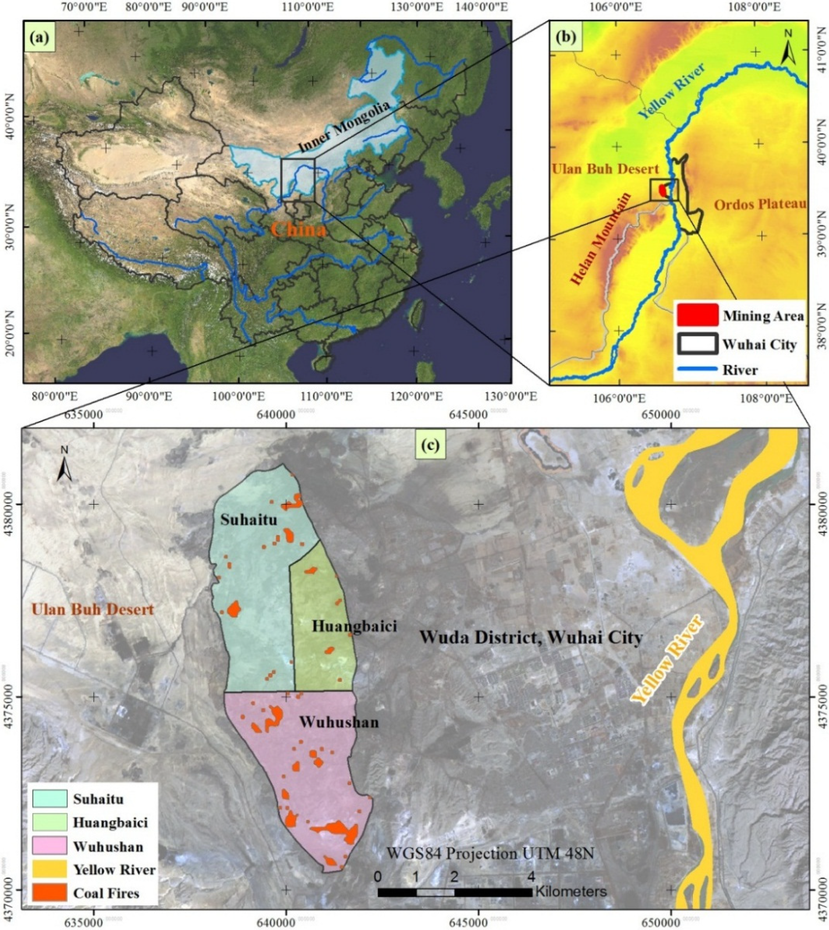
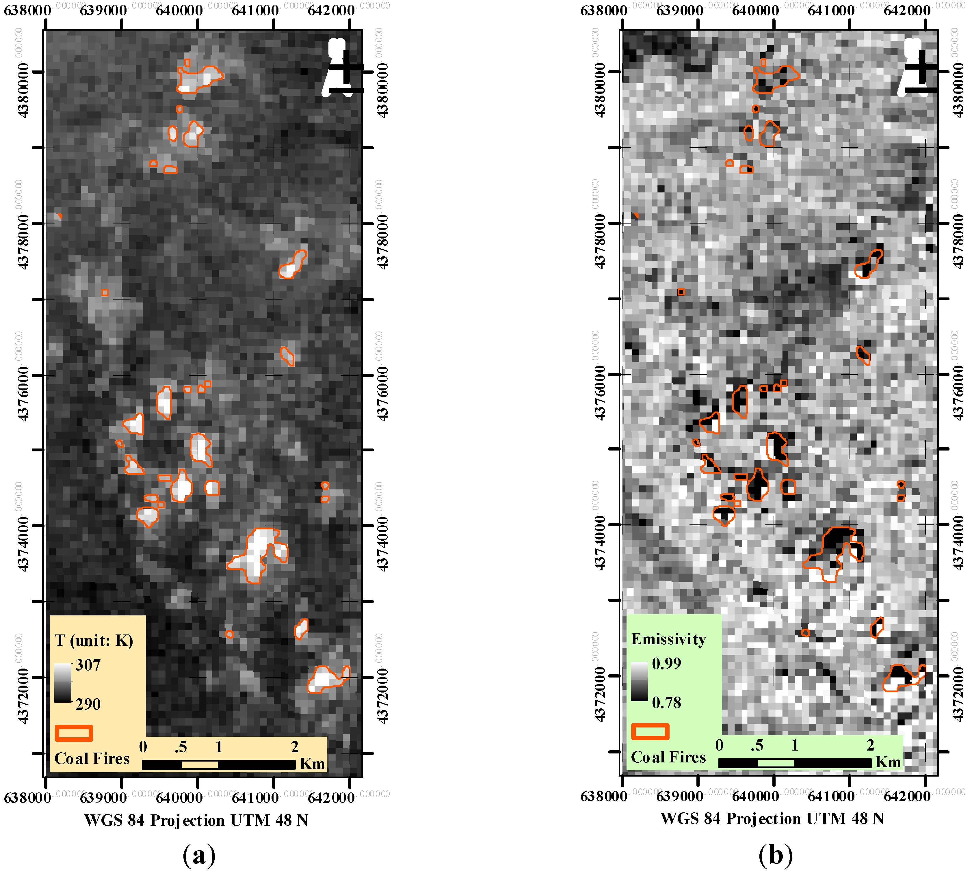
In the Wuda Coalfield, the fire areas with consistently burning fire spots have exhaust gas vents/cracks exposed on the surface that are detectable by remote-based methods and would not be masked by the background temperatures of approximately 300 K. On 27 March 2013 we measured an average temperature of 770 K (497 °C) for the burning fire spots in the field survey, which was conducted to obtain the peak temperatures on the surface. In an experiment of a simulated coal fire [25], it has been reported that the surface radiant temperatures of the coal fire range from 300 °C to 900 °C (573 K–1173 K).

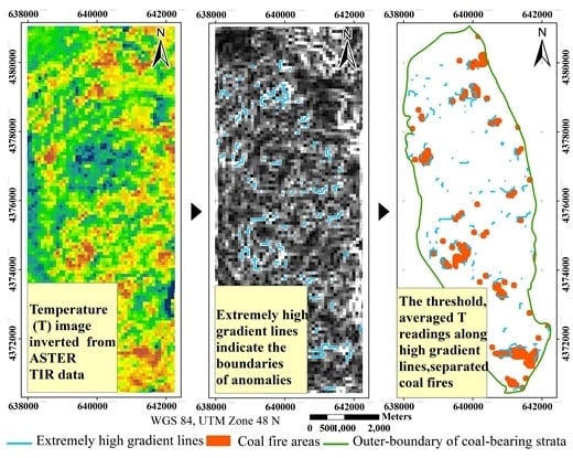
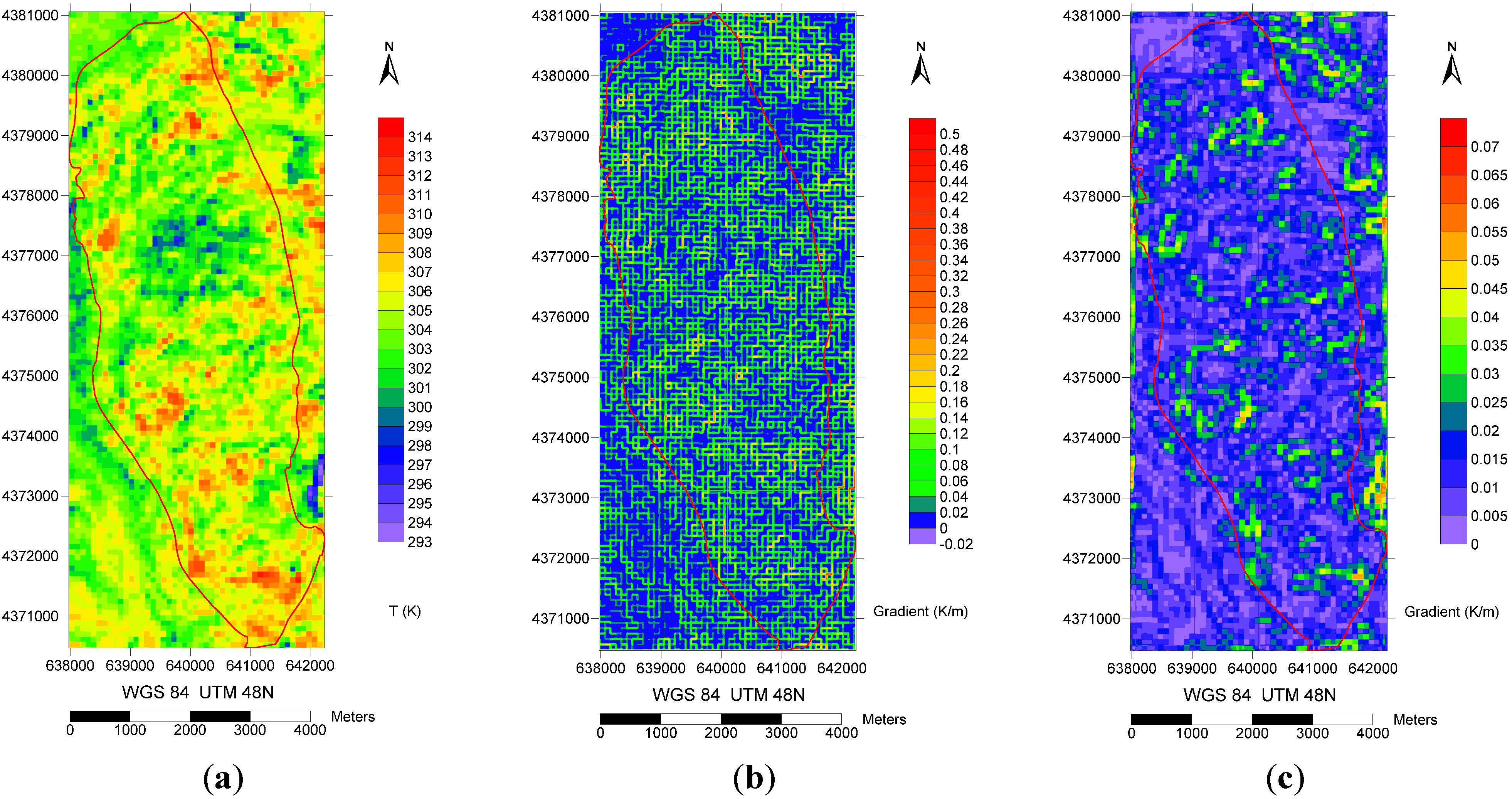
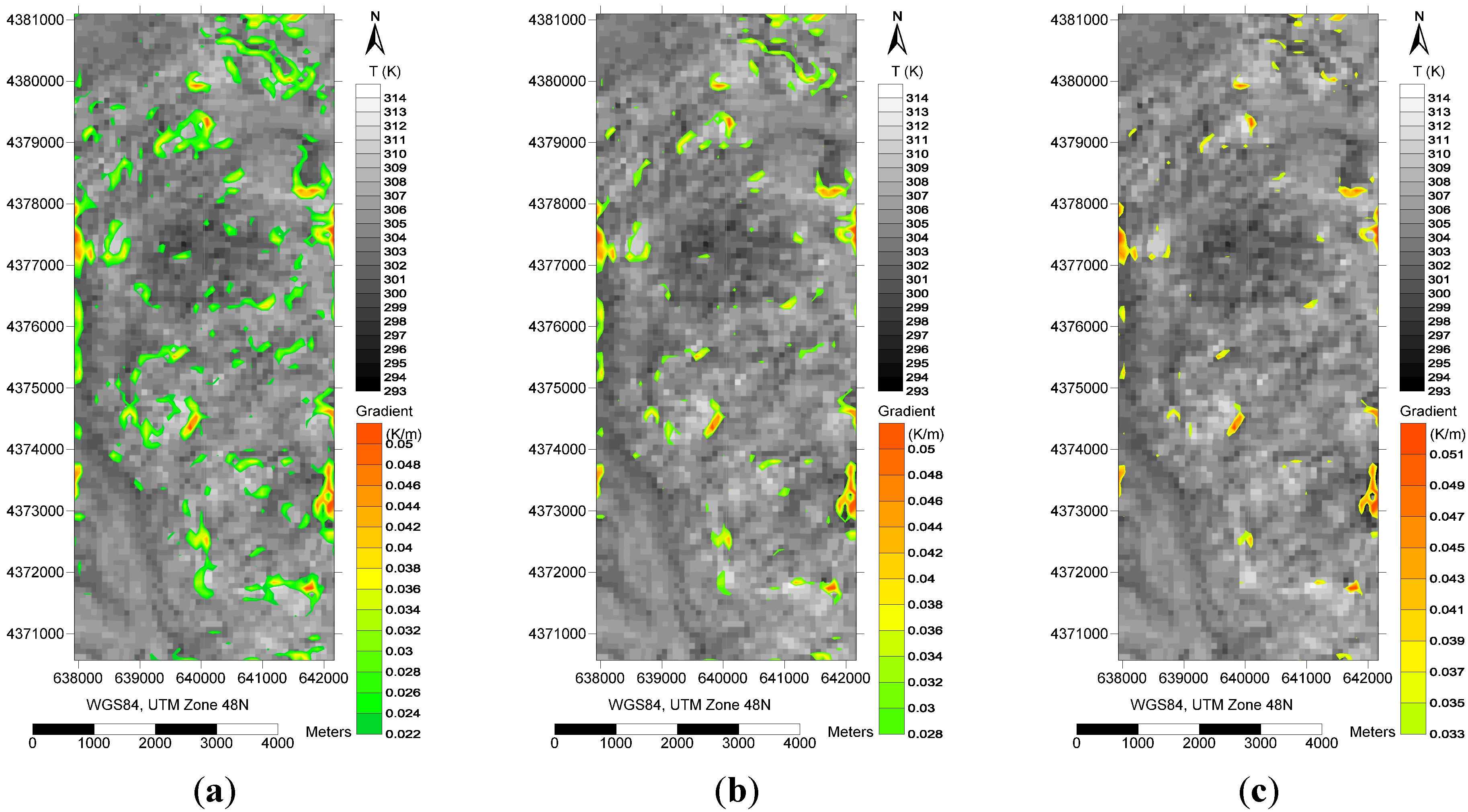
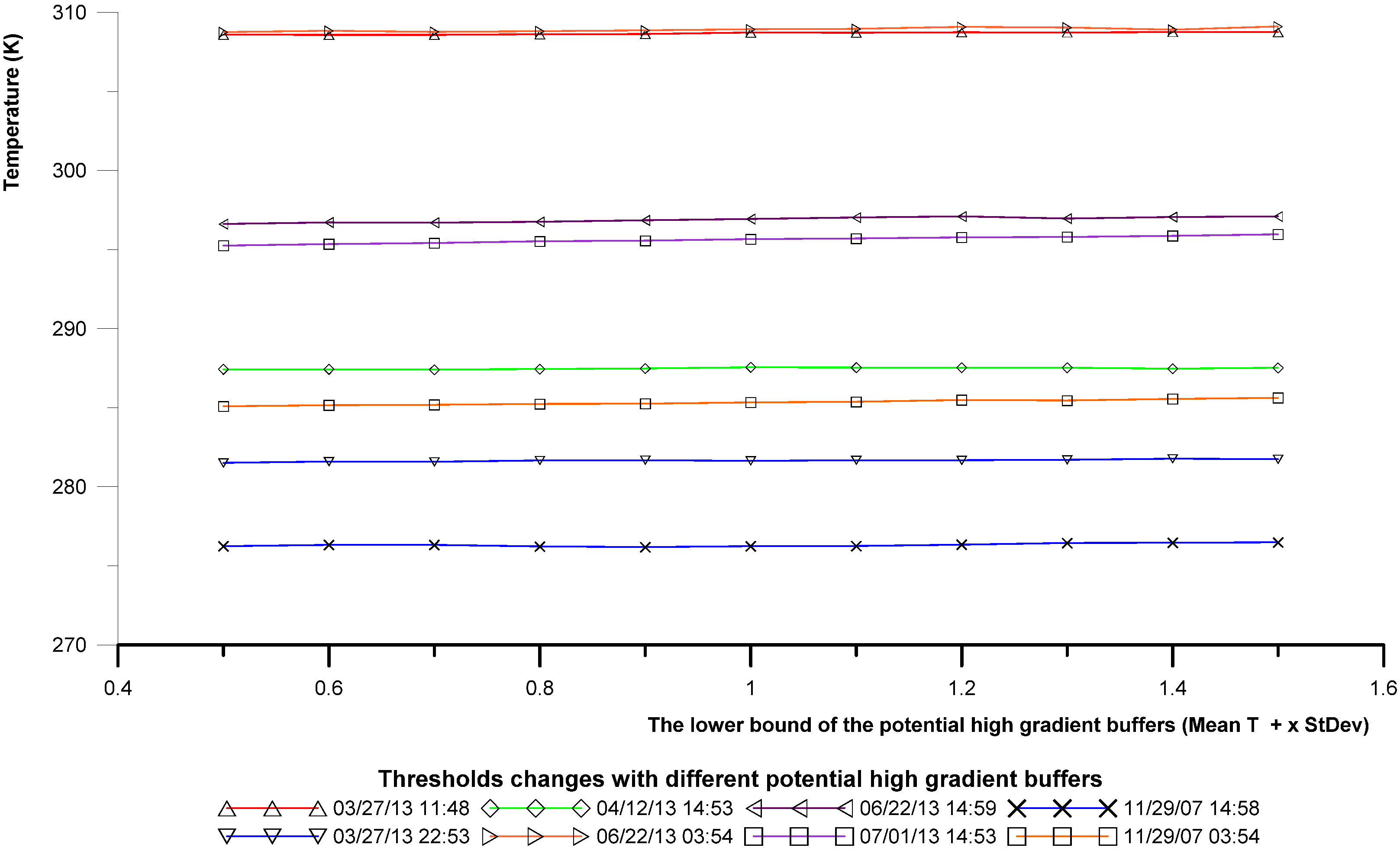
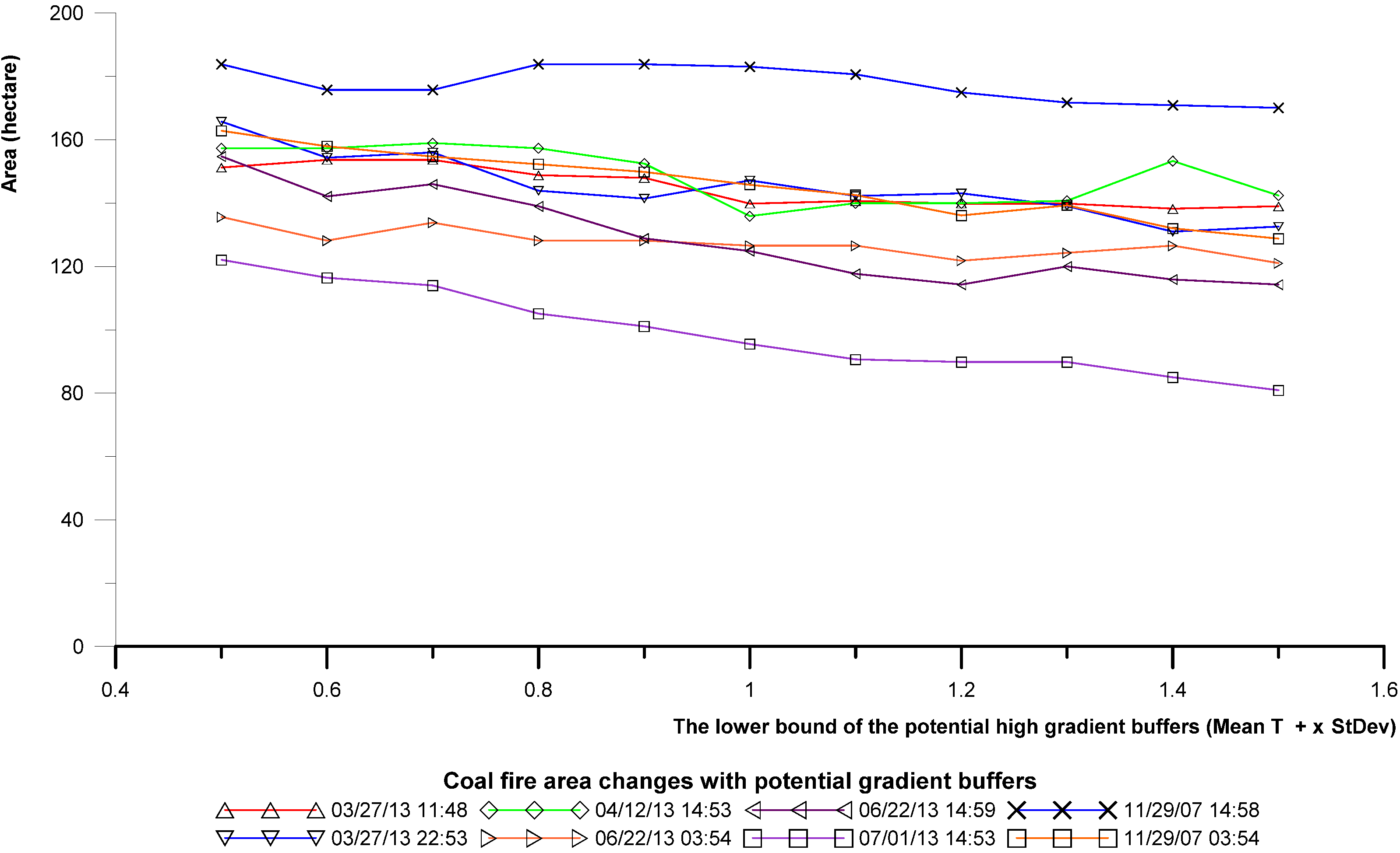
Based on the coal fire’s thermal level and spatial characteristics, this study proposes a self-adaptive gradient-based thresholding method (SAGBT) for coal fire detection in the absence of basic field/geological data. The thermal spatial characteristics of coal fires can be summed up in two aspects: large-scale homogeneity and poor horizontal thermal conductivity. The coal fire risks were induced by the coal properties and environmental conditions [30,31]. In Wuda, the relatively large-scale, homogenous, fine yellow quartz sandstone overlays, and the short and sparse vegetation contribute to the similar thermal conductivity across the region. However, the thermal anomalies induced by coal fire areas do not reach far from the burning centers because they are restricted to the collapsed region, faults, and fissures, which results in poor horizontal thermal conductivity and therefore causes a sharp decrease in the temperature domain on the edge. A given coal fire cannot be far from the burning center, which is supported by the research [32]. 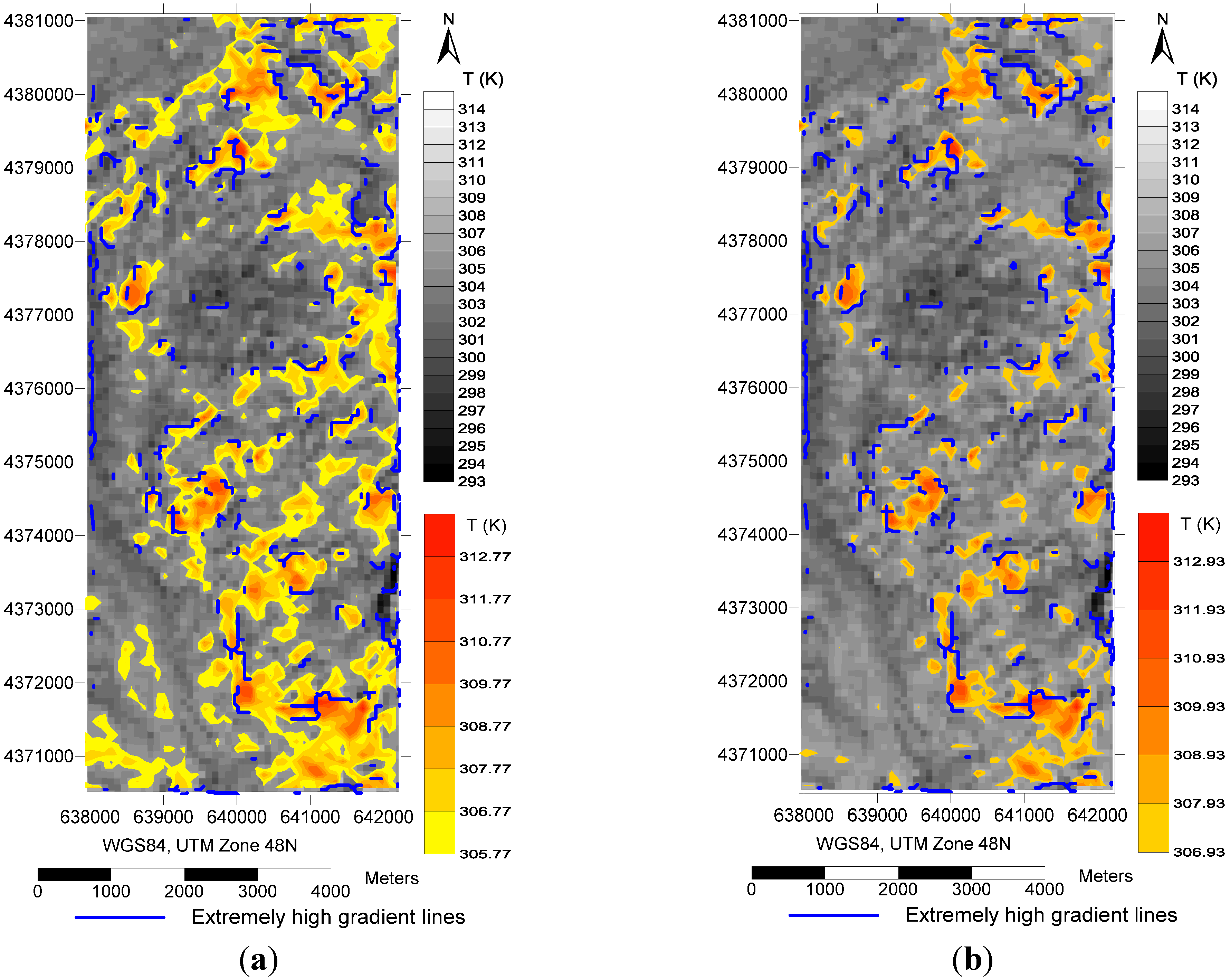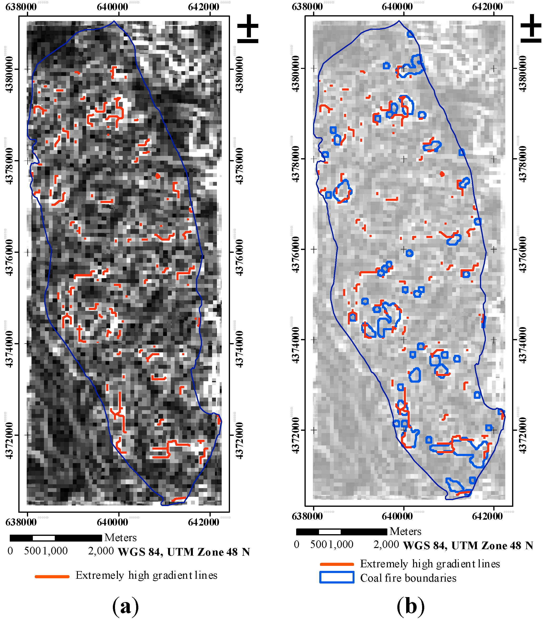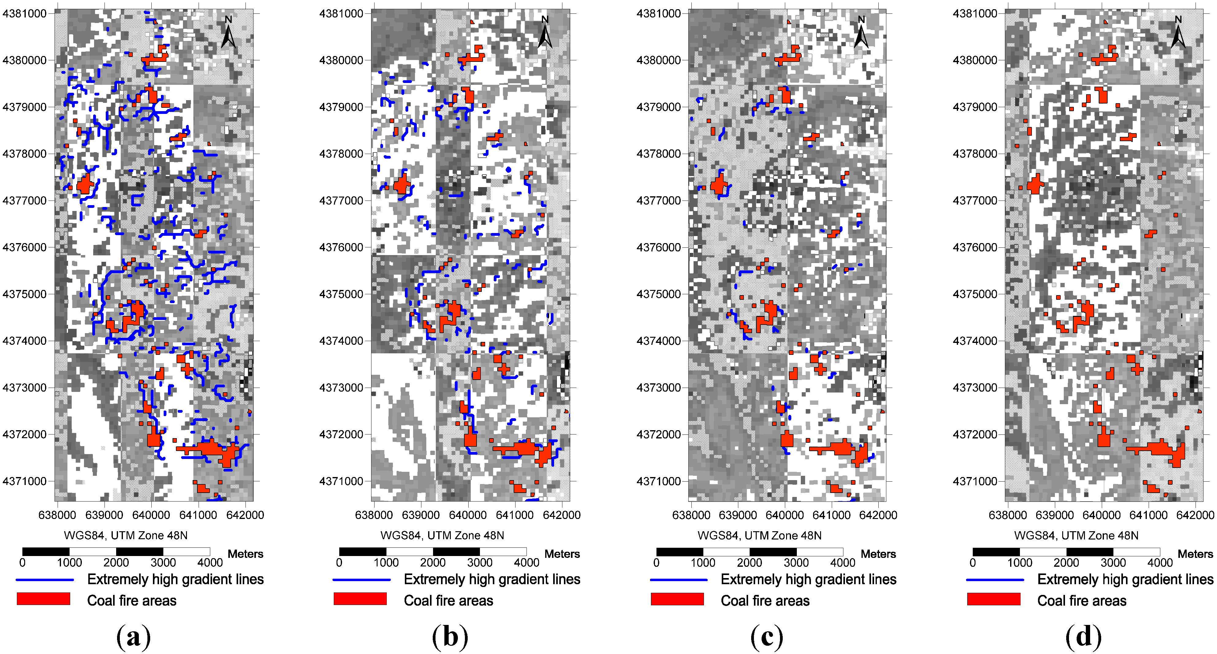In the field, it has been observed that high temperatures do not extend more than 2–3 m from the observed hot cracks; in addition, the temperature gradients are significant, with temperatures varying by more than 500 °C over a distance of less than 20 m [32]. These characteristics of coal fires suggest that the attenuation of temperature along the coal fire’s boundaries generates considerable amounts of spots with extremely high gradient values, resulting in uneven gradients in the integrated pixels (ASTER’s 90 m pixel). This SAGBT method is remote sensing-based, primarily depends on the spatial distribution of the most direct coal fire-induced factor and energy release, and uses the basic outer-boundary of the coal-bearing strata to simply exclude false alarms.

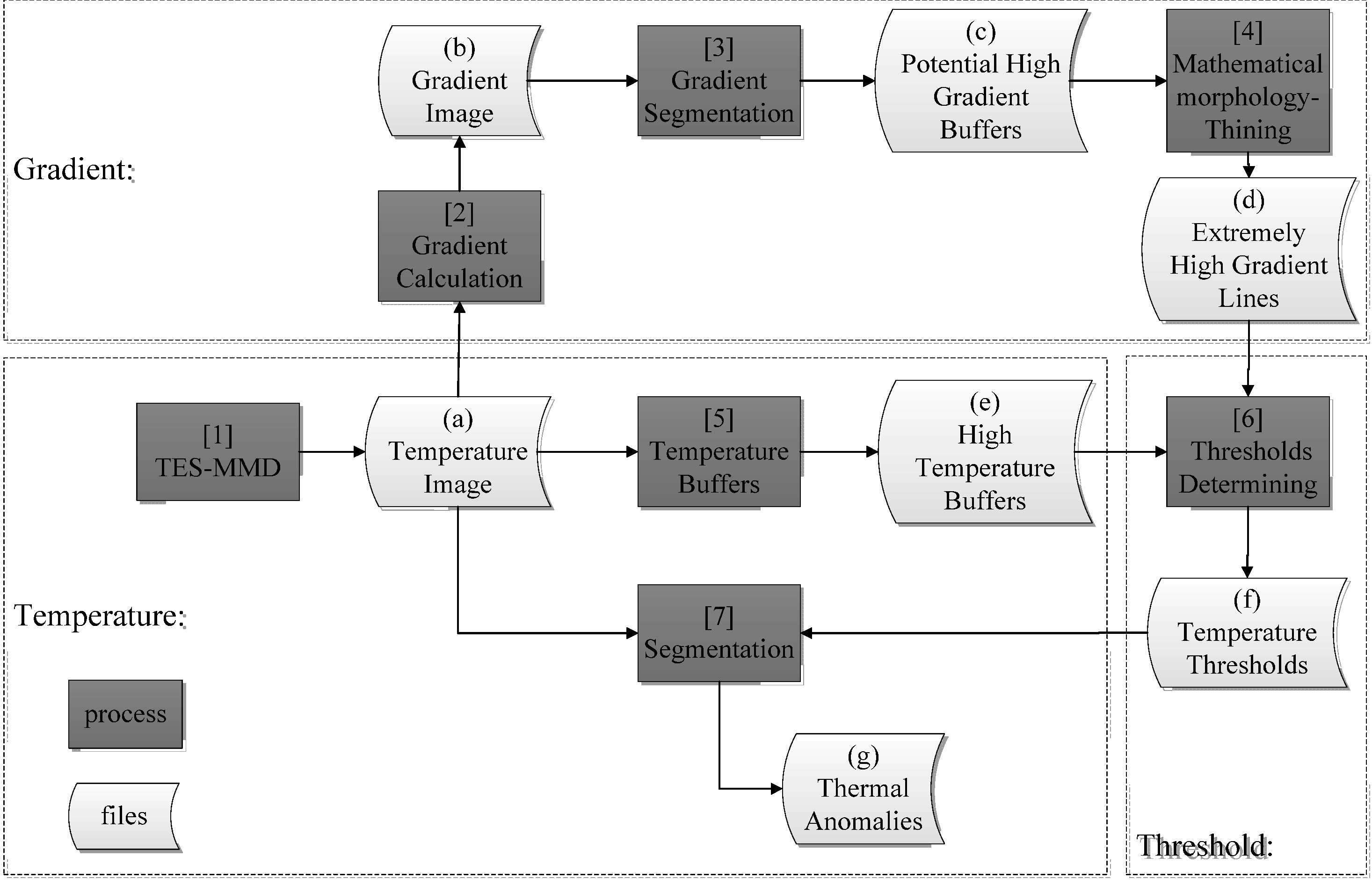
This research addresses the following four key issues in coal fire detection: a temperature retrieval method for the TIR images; a gradient calculation algorithm based on supersampled images to guarantee adequate image matching; a skeletonization method to reduce the gradient buffers to single pixel lines; and the determination of thresholds and related convergence analysis for the SAGBT method.

For monitoring the coal fire changes in the Wuda Coalfield, several authors have successfully evaluated the development/shift of coal fire zones, change in area of fires/fire risk regions, and background radiance variations. Comparing two Landsat datasets (TM and ETM+) for 1987 and 2002, Kuenzer et al. used a maximum likelihood based interactive classification that indicated that the coal-covered surfaces nearly doubled in area in the Wuda Region over a 15-year period [33]. Tetzlaff (2004) compared two ETM scenes (obtained on 25 September 2001 and 28 September 2002) and two BIRD datasets (16 January 2003 and September 2003), and showed that these datasets are capable of detecting major shifts or activity changes in terms of hot coal fire surface anomalies and background radiance variations in the Wuda area [17]. Li et al. (2005) also detected coal fires by a statistical method from 2002 to 2004 based on multi-spectral coal fire demarcation [34]. Yang et al. (2005) normalized two Landsat-7 ETM+ images (obtained on 12 August 1999 and 22 September 2002) and extracted thermal anomalies with different surface environmental parameters. The comparison proved that the coal fire area in Wuda enlarged greatly in those years [35]. Chen et al. (2007) processed two scenes of Landsat-7 TM and ETM+ data for 1992 and 2002 and separated coal fires as thermally anomalous areas lying in or around coal containing regions with ancillary data and other images [36]. By three-dimensional mapping and comparison analysis, they discovered that the coal fire changes in the Wuda Coalfield from 1997 to 2002 increased from 16,200 m² to 38,610 m² [36]. Kuenzer et al. (2008) introduced a multi-temporal coal fire mapping technique for all major coal bed fires in the Wuda coal field based on field observations and high-resolution satellite data [27]. They monitored coal fire developments such as shrinkage and change in area for different coal fire zones and proposed a protection of valuable coal resources in the Wuda syncline [27]. Kuenzer et al. (2012) applied the same approach for coal fire change detection from 2000 to 2005 and in 2010 and showed that over the past 10 years a trend can be observed showing underground fires moving eastwards [29]. Jiang et al. (2010) monitored coal fires for 1989, 2001, and 2005 in the Wuda Coalfield, and analyzed the spatial distribution, rate of change, and extending direction of coal fires. The results indicated an annual fire area increasing at the rate of 61.3 × 10³ m² (2.48% of total area) [37]. Kuenzer et al. (2008) used multi-diurnal MODIS data, especially bands 20, 32, and band ratio, and proved that MODIS has a high potential for the detection of coal fire zones and coal fire hotspots, as well as for regular thermal monitoring activities; however, it is difficult to detect coal fire size changes or intensity changes from a comparison of only two MODIS data sets [8].

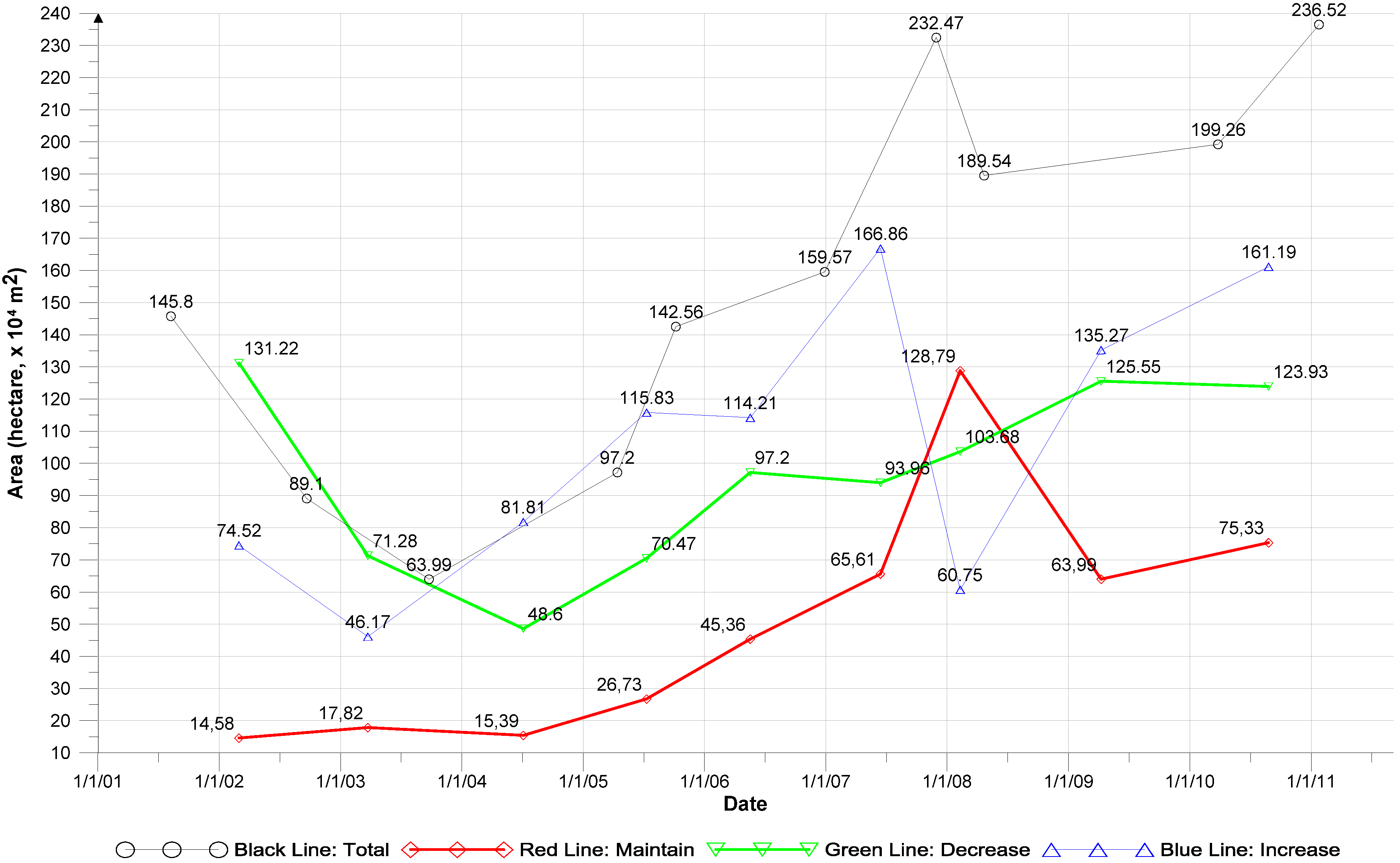
This coal fire change detection generally compared 2–3 scenes of TIR images, and lacked co-analysis with the coal productions. In addition, there is no published research on the use of a remote sensing method to perform a change detection analysis for a continuous time period spanning more than 10 years in the Wuda Coalfield. Our change detection adopted the no-interactive coal fire thresholding algorithm, SAGBT, for estimating the decadal change. On the basis of experiments and validation, this algorithm demonstrated convergence and matching of the observed coal fire areas. Since the thresholds are self-adapted based on the thermal spatial distribution of different images obtained in different seasons, this method provides an opportunity to monitor long-term coal fire changes using the TIR images from ASTER sensor. Our research also explores the possibility of estimating the CO₂ emissions due to coal fire propagation using change detection results. A temporal animation performed in Google Earth is used to dynamically visualize these changes. As an application and an estimation of efficiency for the SAGBT, we analyzed 10 years of change in coal fires via a time-series analysis.

2. Study Area and Data

2.1. Study Regions

The Wuda Coalfield is located in Wuhai City in the southwestern Inner Mongolia Autonomous Region of China (Figure 1a). The area is on the northern edge of the Helan Shan mountain range, west of the Ordos Plateau, and is located less than 10 kilometers from the western banks of the Yellow River and less than 10 kilometers from the southern edge of the Ulan Buh Desert (Figure 1b). The coalfield is bounded by the latitudes 39°28'21.15"N and 39°34'6.01"N and the longitudes 106°36'21.83"E and 106°39'15.53"E. The altitude varies from 1090 m to 1380 m (average 1207.4 m) according to the data from the Shuttle Radar Topographic Mission (SRTM). The study area closed by the coalfield’s outer boundary in Figure 1c covers approximately 27.59 km² and includes the following three mines: Suhaitu, Huangbaici, and Wuhushan.

Figure 1. Location of the Wuda Coalfield. (a, b) The study area is in Inner Mongolia, China. (c) The Wuda Coalfield includes three coal mines, which are characterized by an “ear-shaped” syncline. The red polygons depict the coal fires for 22 June 2013, 22:58 (local time: GMT+8), which were extracted by our SAGBT method.

2.2. Remote Sensing Data for Algorithm Development

This research used images from the ASTER sensor. ASTER is a payload of NASA’s Terra satellite and acquires images at a 15-m spatial resolution using four spectral bands in the visible and near-infrared regions (VNIR) (bands 1–3 and 3N) of the electromagnetic spectrum. ASTER has five spectral bands in the thermal infrared (TIR) range (bands 10 to 14, from 8.125 to 11.65 μm), which produce images at a 90-m spatial resolution. The thermal images from ASTER can be used to retrieve the surface temperature and surface spectral emissivity and have been used in a wide variety of applications, including environmental monitoring, geological mapping, and hazard prediction.

We attempted to obtain the daytime/nighttime ASTER TIR image pairs to represent the thermal distribution for different seasons, and then the corresponding Level-1B products (Table 1) were processed by a temperature emissivity separation algorithm. However, there is only one pair of daytime/nighttime images available over the Wuda Coalfield in ASTER’s historical inventory, which includes data for 29 November 2007 (winter images). Thus, we tasked ASTER with acquiring images over the study site during the spring and summer of 2013. Two day/night image pairs for the same date were acquired on 27 March 2013 (close to the spring equinox) and on 22 June 2013 (summer solstice) to calibrate our algorithm. The nighttime TIR images for 12 April 2013 and 1 July 2013 were also obtained as supplementary data to compare the nighttime coal fire delineation with the closest nighttime images. The historical image pair for 29 November 2007 (winter) was used to illustrate the method when applied to a different time of the year/season. An additional scene for 21 September 2002 was used as a comparison to work performed by others. The published ancillary data and the geological data from the literature [38] were used to generate a coal fire risk area composed of the outcrop of the lowest coal seam and the over-thrust fault line for the removal of false alarms. All the TIR images were cropped by this outer bounding box of the Wuda Coalfield. Unless specified, the TIR images are these cropped images in the following sections. In the subsequent paper, “Part 2, Validation and Sensitivity Analysis,” we report comparisons using LST measurements during the ASTER overpass during the simultaneous field campaigns on 27 March 2013 and 22 June 2013.

Table 1. ASTER scenes for algorithm development.

**Table 1.** ASTER scenes for algorithm development.
Acquisition Date, Time (month/day/ year time UTC)	Day/Night
03/27/2013 03	Day
03/27/2013 14	Night
04/12/2013 14	Night
06/22/2013 03	Day
06/22/2013 14	Night
07/01/2013 14	Night
11/29/2007 03	Night
11/29/2007 14	Day
09/21/2002 14	Night

2.3. Remote Sensing Data for Decadal Change Detection (2001 to 2011)

Nighttime data are ideal for this study because solar heating of the Earth’s surface contributes significantly to the total radiant energy flux during the daytime. In addition, topographic unevenness and land cover/land use differences may cause differential solar heating during the daytime [2]. Therefore, the nighttime thermal infrared images can decrease the impact of differential solar heating and differences in topography and land cover, such as bare soil and desert [39]. However, because of the limited availability of nighttime ASTER data in the Wuda Coalfield, we have used five sets of daytime data acquired in 2001, 2003, 2005, 2006, and 2010 to make up for the nighttime ASTER data gap. An algorithm developed by combining both daytime and nighttime ASTER data is also a unique aspect of this research. Table 2 provides the scene IDs and dates of the ASTER images used in the study. In this paper, we used a simplified scene ID to identify these ASTER images, keeping the first eight digits to represent the year, month, day, and hour (local time: UTC+8 hours).

Table 2. ASTER scenes used in change detection.

**Table 2.** ASTER scenes used in change detection.
Aster Scene ID ¹	Acquisition Date (dd/mm/yyyy)	Day/Night
ASTL1B_0108080402180108190577	8 August 2001	Night
ASTL1B_0209211454220210140292	21 September 2002	Night
ASTL1B_0309240347540310110308	24 September 2003	Night
ASTL1B_0504131458440504160548 ²	13 April 2005	Night
ASTL1B_0510060353310510080444	06 October 2005	Night
ASTL1B_0612280354140701010054	28 December 2006	Night
ASTL1B_0711291458560806290389	29 November 2007	Day
ASTL1B_0804211459100804240676	21 April 2008	Night
ASTL1B_1003260354351003290102	26 March 2010	Night
ASTL1B_1101241458341101270384	24 January 2011	Night
ASTL1B_0108080402180108190577	23 December 2013	Day

¹ ASTER Scene IDs follow the image identification system used by the ASTER GDS, Japan Space Systems. The first 12 digits represent the date and time (UTC) of data acquisition (yymmddHHMMSS), in the following we used this shortened Scene IDs with first 8 digits; ² This scene is a repaired image. The original image had a triangle-shaped data gap in the northeast part of the image, which occupied 2% of the coalfield area and influenced 4.21% and 2.83% of the coal fire area in the previous and next images, respectively. To complete the change detection, this gap was filled with mean values of pixels from the two images before and after this acquisition date. We estimated the fire area influenced by this data gap would not change the trend of the fire area.

2.4. Coal Production Data for the Wuda Coalfield

The coal production data for the last decade were collected from published coal industrial yearbooks (SACMS 2001–2011) and a news report from the local official newspaper, Inner Mongolia Daily [40,41].

3. Preliminary Data Preprocessing and Analysis

3.1. Atmospheric Correction

The Thermal Atmospheric Correction module in ENVI^®, which incorporates an in-scene atmospheric compensation (ISAC) algorithm [42], was applied to the Level 1B ASTER images prior to their incorporation into the temperature inversion workflow. This algorithm has been widely used on multispectral thermal infrared and hyperspectral images [43]. The methods based on ISAC use the actual at-aperture radiance data in the hyperspectral image cube to remove the atmospheric influence associated with atmospheric transmissivity, up-welling path radiance, and down-welling sky irradiance. ISAC does not use any site-specific weather data, such as temperature, relative humidity, or air pressure, which makes this algorithm suitable for studying remote sites, such as our study site.

3.2. Land Surface Temperature and Land Surface Emissivity Retrieval

A variety of methods and algorithms has been proposed to retrieve the Land Surface Temperature (LST) and Land Surface Emissivity (LSE) from thermal infrared data. Methods to retrieve the LST that compensate for the emissivity effects can be classified into the following three categories: Single-channel methods, two-channel or split-window methods, and two-angle methods [44,45,46]. The single-channel methods rely on accurate atmospheric profiles [47], which are unavailable for our study site and image acquisition dates. The popular split-window method requires prior knowledge of the emissivity. The two-angle method requires one measurement at a significantly longer atmospheric path and depends on knowledge of the angular distribution of the surface emissivity [48,49]. These methods are unsuitable for complex land surfaces [45]. Emissivity methods have been proposed to estimate the LSE or its shape, and common LSE algorithms include the reference channel method [50], normalized emissivity method (NEM) [51], alpha residuals [52], thermal spectral indices [53], and spectral ratio [54]. A complex temperature emissivity separation (TES) technique for the ASTER data has been proposed [55], which combines multiple modules, including approaches based on NEM, relative emissivity ratio, and maximum minimum difference (MMD), with an absolute accuracy of 1–4 K and a relative accuracy of 0.3 K [55].

In this study, we used the TES-MMD method considering the following: (1) the availability of multispectral capabilities in the thermal infrared region of the ASTER sensor and (2) the lack of surface emissivity data and historical meteorological data, which are required when using the single-channel and split window methods.

3.3. Reasons for Gradient-Based Thresholding: Seasonal and Diurnal Variations in the Thermal Distribution

The LST was inverted through the TES-MMD process. Then, these thermal distributions were mapped in color-filled contour maps to demonstrate the seasonal and diurnal (day/night) variations in the thermal patterns. First, we compared the ASTER-derived thermal distribution for the nighttime images acquired on the following four dates: 27 March 2013, 22 June 2013, 21 September 2002, and 8 December 2007. These dates are close to the spring/autumnal equinoxes and the summer/winter solstices and can adequately represent the four seasons.

We mapped the thermal levels to a uniform color scale from 260 K to 310 K (Figure 2). Green tones predominate for the nights of the spring/autumnal equinoxes, with average temperatures of 278.06 K for 27 March 2013 and 283.69 K for 21 September 2002. On the night of 22 June 2013 (summer solstice), the map shows a warmer tone, corresponding to a mean LST value of 293.62 K. The mean temperature for the night of 8 December 2007 (close to the winter solstice) was 268.75 K, and cold blue tones predominate.

Figure 2. Thermal distribution over the Wuda Coalfield for the nighttime ASTER images acquired on the following four dates: (a) 27 March 2013; (b) 22 June 2013; (c) 21 September 2002; and (d) 8 December 2007.

For the day/night analysis of the thermal distribution patterns, we then assumed that the thermal levels during the spring and autumnal equinoxes are similar, and we chose 27 March 2013 to represent the spring and fall considering the limited availability of ASTER images (Figure 3a). The image pair for 22 June 2013 (summer solstice) represented the summer (Figure 3b) and the image pair for 29 November 2007 represented the winter season (Figure 3c). The differences in the mean temperatures between the day and night can be observed as follows: 26.55 K for spring (day = 304.61 K, night = 278.06 K); 11.06 K for summer (day = 304.68 K, night = 293.62 K) and 11.15 K for winter (day = 280.18 K, night = 269.03 K). Briefly, the day and night temperature difference during the spring is more dramatic than during the winter and summer. For the winter map, the fire areas present a brighter contrast compared with the background, considering the relatively lower mean LST. In addition, the temperatures for the winter map are distributed more similarly between the day and night than in other seasons. We observed a general seasonal variability in the daytime and nighttime thermal levels. The thermal anomalies, however, showed similar daytime and nighttime spatial distribution patterns for a given date, thus allowing for the retrieval of the anomalies during the daytime and nighttime.

Anomaly identification using a single threshold has shown limited success in separating the thermal contributions from the background; thus, a relative or dynamic threshold approach is proposed. Our temperature gradient-based thresholding model assumes that the thermal gradient distribution should be stable within a short period, although the distribution of high temperatures is significantly different considering summer/winter or daytime/nighttime.

Figure 3. Thermal distribution map of the day/night pairs for the same date during different seasons representing spring/fall, summer, and winter. The images were acquired on (a) 27 March 2013, 11:48 A.M.; (b) 22 June 2013, 11:54 A.M.; (c) 29 November 2007, 11:54 A.M.; (d) 27 March 2013, 22:53 P.M.; (e) 22 June 2013, 22:59 P.M.; and (f) 29 November 2007, 22:58 P.M.; Local Time: GMT+8.

3.4. Thermal Anomalies and the Definition of Coal Fire Areas

It was observed that the temperature of a coal fire area during the combustion stage was higher than 61 °C (334 K) [31]; the average temperature at cracks is 237 °C (510 K) [32]. By summarizing multiple coal fire studies, the temperatures around the fire sources have been determined to range from 150 °C (423 K) to 250 °C (523 K) [2]. The coal fire in the Wuda Coalfield initiated from spontaneous combustion spots, propagated along the cracks, and merged into a plane [31]. Therefore, not all the pixels were saturated, especially at the hot spot and along the thermal conducting cracks, where the pixels are a mixture of fire zones and lower temperature surfaces. In certain areas, the pixel-integrated temperature was below the fire source (423 K–523 K, 150 °C–250 °C) and the minimum temperature values for spontaneous combustion (334 K).

A criterion to determine the threshold to separate thermally anomalous pixels (hot spots) from the background pixels is essential, but using certain temperatures does not work due to different locations, coal properties, and environmental conditions. Therefore, we defined coal fire areas as temperature anomalies derived from the TIR images restricted by strip boundaries, in which the LST sharply decreases from the high temperature burning centers to a low temperature background temperature. We used this definition to flag pixels with temperatures above a threshold, which was defined as an average temperature reading from the high temperature buffers (with a range greater than 1.0 σ from the mean) and along the extremely high gradient lines (thinned from the potential high gradient buffers segmented within the lower bound range 0.5–1.5 σ and the upper bound 3.2 σ, with σ as the standard deviation), as coal fire areas. The potential high gradient buffers are redundant in screening out the homogeneous low gradient background and the extremely high gradient points resulting from the burning spots. The high temperature buffers were defined by a segment value of 1.0 σ from the mean. Because we observed that the thermal anomalies segmented by 1.6 σ fit the surveying map of 21 September 2002 very well, we considered a 0.6 σ tolerance factor to our 1.0 σ as a lower bound to compensate for the differences caused by uneven solar heating, variations in slope, aspect, and vegetation cover, which can mask the thermal anomalies related to coal fires, according to the field survey observations [32].

4. Algorithm of SAGBT

4.1. The Workflow of SAGBT

As shown in the algorithm flow chart (Figure 4), the source of the data is a temperature image (Figure 4a) derived from a temperature retrieval method. A gradient calculation method (Figure 4 “[2]”) was used to profile the magnitude of the difference among the adjacent pixels. The gradient image (Figure 4b) recorded the significance of the temperature variation. To connect extremely high gradient pixels, we used two procedures. First, we segmented the gradient images by a pair of lower and upper bounds, such as 1.0–3.2 σ, and retained the relatively high gradient values (see the process in Figure 4 “[3]”). These intermediate segmented gradient pixels around the high temperature anomalies form ring shaped areas, called potential high gradient buffers (Figure 4c). Then, a mathematical morphology thinning method (see the process in Figure 4 “[4]”) was applied to skeletonize these ring areas into lines with a width of one pixel, called extremely high gradient lines (Figure 4d).

Figure 4. Flow chart of the gradient-based thresholding algorithm. The gray rectangles are processing modules (“1” to “7”). The bent rectangles are temporary or final files (“a” to “g”).

Another branch of this method is to segment the high temperature areas. These areas can prevent the reading of low temperatures from cold areas along the extremely high gradient lines. We used a relative board segment value of 1.0 σ to guarantee a high-temperature area (defined as high temperature buffers in Figure 4e), which was used to match the 11 extremely high gradient skeletons to obtain 11 different intermediate thresholds; each threshold equals a mean temperature along an extremely high gradient skeleton. Finally, the average value of the 11 intermediate thresholds is considered as the threshold (Figure 4f) for a temperature image. Among these image processes, a basic outer boundary of the coal-bearing strata is used to subset the image within the coalfield to narrow down the target coal fire areas and remove false alarms. The key steps (including the gradient calculation, potential high gradient buffer segmentation, high temperature buffer segmentation, mathematical morphology thinning, and threshold identification) are specifically presented in the following sections. In this study, these automatic fire detection modules were implemented using Interactive Data Language (IDL).

4.2. Gradient Calculation

The thermal images used in this study were supersampled to facilitate geometric matching between the VNIR and TIR images. During the supersampling, one original TIR-derived pixel was resampled into 36 pixels with a single LST value. For these supersampled datasets, we applied a gradient filter structure modified from the common Sobel filter and expanded the structure to calculate pixels for intervals of six pixels. The convolution structures incorporated into the methodology are presented in Equations (1) and (2), as follows:

G_{x} = \frac{\frac{1}{4} [\begin{matrix} - 1 & 0 & 0 & 0 & 0 & 0 & + 1 \\ 0 & 0 & 0 & 0 & 0 & 0 & 0 \\ 0 & 0 & 0 & 0 & 0 & 0 & 0 \\ - 2 & 0 & 0 & 0 & 0 & 0 & + 2 \\ 0 & 0 & 0 & 0 & 0 & 0 & 0 \\ 0 & 0 & 0 & 0 & 0 & 0 & 0 \\ - 1 & 0 & 0 & 0 & 0 & 0 & + 1 \end{matrix}]}{90 m}

(1)

G_{y} = \frac{\frac{1}{4} [\begin{matrix} - 1 & 0 & 0 & - 2 & 0 & 0 & - 1 \\ 0 & 0 & 0 & 0 & 0 & 0 & 0 \\ 0 & 0 & 0 & 0 & 0 & 0 & 0 \\ 0 & 0 & 0 & 0 & 0 & 0 & 0 \\ 0 & 0 & 0 & 0 & 0 & 0 & 0 \\ 0 & 0 & 0 & 0 & 0 & 0 & 0 \\ + 1 & 0 & 0 & + 2 & 0 & 0 & + 1 \end{matrix}]}{90 m}

(2)

\vec{G} = G_{x} x + G_{y} y

(3)

G_{M a g n i t i t u d e} = | \vec{G} | = \sqrt{G_{x}^{2} + G_{y}^{2}}

(4)

Only the magnitude of the gradient was retained, considering our assumption that the extremely high gradient values are strongly correlated to the coal fire’s edges. The gradient orientation was not observed to contribute to the threshold calculation. Figure 5b shows the high gradient lines distributed along the 90 m pixel boundary when the common Sobel filter was applied to the supersampled image. When using our extended Sobel filter, the gradient image calculated by Equations (1)–(4) showed smooth and more reasonable bright lines in Figure 5c around high temperature areas in Figure 5a.

Figure 5. Gradient calculations from the temperature images: (a) temperature image for 27 March 2013 (unit: K); (b) gradient image resulting from the original Sobel method (the horizontal and vertical lines with high gradient values match the pixel edges of the original 90 m resolution thermal image (unit: K/m); (c) gradient image divided by our expanded Sobel convolutions (unit: K/m).

4.3. Potential High Gradient Buffers

In the gradient counter map, we found extremely high gradient centers located at the center of the small closed counters that were distributed into rings (Figure 6), which form the potential boundaries of coal fires. Thus, an intermediate result consisting of the potential high gradient buffers segmented by a lower bound and higher bound was used to include these extreme centers. These buffers were then skeletonized to the extremely high gradient lines to trace the extremely high gradient centers.

These potential high gradient buffers became thinner and shorter as the lower and higher segmentation bounds became narrower. As shown in Figure 7, narrower potential high gradient buffers allow for more accurate threshold identification, but fewer pixels are available to define the shape of the coal fire area. Through visual interpretation, we found that the extremely high gradient values surrounding the thermal anomalies range from 0.03 to 0.05 (Figure 7a–c). Values higher than 0.05 correspond to strong burning areas and values lower than 0.03 correspond to areas with stable temperature. Thus, we proposed wider potential high gradient buffers ranging from 0.5 σ to 3.2 σ to include these extremely high gradient centers.

Figure 6. Potential high gradient buffers compared with a rough thermal anomalies map. (a) Generally declares the range of digital values in each image greater than the mean value plus the 1.6 Standard deviation (Mean + 1.6 σ) as thermally anomalous; (b) gradient counter map, mapped with digital values ranging from Mean + 1.0 σ to Mean + 3.2 σ; (c) overlay map with the rough anomalies map and gradient counter map.

Figure 7. Potential high gradient buffers segmented using a different lower segment bound for the 27 March 2013 image: (a) segment values ranging from 0.5 to 3.2 σ; (b) values ranging from 1.0 to 3.2 σ; and (c) values ranging from 1.5–3.2 σ.

4.4. High Temperature Buffers

Figure 8a,b illustrate that the majority of the extremely high gradient lines are located along the edges of the potential high temperature areas. However, a small number of those lines were located around low temperatures, which could lead to an incorrect identification of the coal fires. These false positives were eliminated by overlaying the high temperature buffers to restrict the thinned gradient lines within the high-temperature areas. The survey data indicated a match between the coal fire areas and the temperature images, particularly for temperatures above a threshold range 1.6 σ to 2.0 σ from the mean value. Therefore, the high temperature buffers were defined using an extended segment value of the mean temperature plus 1.0 σ, which is an empirical value with sufficient tolerance in the temperature domain. As shown in Figure 8b, the 1.0 σ segmentation threshold produced high temperature buffers. The statistics regarding these buffers for multiple ASTER scenes are presented in Table 3.

Figure 8. Segmented high temperature buffers for 27 March 2013, 11:54 (Local Time: GMT+8). (a) High temperature buffers segmented by the mean value plus 0.5 σ; (b) high temperature buffers segmented by the mean value plus 1.0 σ.

Table 3. Mean and standard deviation for the temperature images from multiple ASTER scenes.

**Table 3.** Mean and standard deviation for the temperature images from multiple ASTER scenes.
No.	Date Time of Acquisition	Day/Night	MEAN T (K)	STDEV, σ	Mean + 0.5 σ	Mean + 1.0 σ	Mean + 1.6 σ	Mean + 2.0 σ
1	2013/03/27 03	Day	304.61	2.31	305.77	306.93	308.32	309.25
2	2013/03/27 14	Night	278.06	1.90	279.01	279.96	281.09	281.85
3	2013/04/12 14	Night	283.92	1.95	284.90	285.87	287.04	287.82
4	2013/06/22 03	Day	304.68	1.91	305.63	306.59	307.73	308.50
5	2013/06/22 14	Night	293.62	1.39	294.32	295.01	295.84	296.40
6	2013/07/01 14	Night	292.35	1.51	293.10	293.86	294.76	295.36
7	2007/11/29 03	Day	280.18	2.46	281.41	282.64	284.12	285.10
8	2007/11/29 14	Night	269.04	3.69	270.88	272.73	274.94	276.41

4.5. Mathematical Morphology Thinning and Extremely High Gradient Lines

We applied mathematical morphology thinning to trace the extremely high gradient lines (boundary lines) connecting the extremely high gradient pixels. The mathematical morphology method is based on set theory, lattice theory, topology, and random functions for the analysis of geometrical structures [56]. Thinning is a mathematical morphology method that is particularly useful for skeletonization. The method preserves the shape’s connectivity and the overall shape’s dimensions and reduces the line width by removing the boundary pixels that are not shape endpoints. The thinning method, when applied to a binary image, iterates the algorithm and removes boundary pixels (pixels that have more than one non-zero neighbor pixels), as long as doing so does not create locally disconnections (i.e., split the non-zero image into two parts), until the binary image converges into lines one pixel in width [57]. The thinning method totally defined eight structuring elements 3 × 3 in size. Structuring elements are used to check if a central pixel and its eight neighbors in a binary image fit one of these eight structuring elements. If one structuring element fits, the central pixel is removed (assigned as zero). The process is repeated in a cyclic fashion until the thinning produces no further change. The final result is also a binary image, a connected skeleton one pixel in width [57].

In the SAGBT algorithm, the potential high gradient buffers were skeletonized to lines one pixel in width, or extremely high gradient lines, corresponding to the high gradient pixels in the gradient image (Figure 9a). The spatial confirmation between the extremely high gradient lines and the extremely high gradient pixels facilitates the delineation of the coal fire boundaries. In the following, we overlaid the extremely high gradient lines onto the corresponding high temperature buffers and retrieved the average temperatures. These averages were used as thresholds to separate the fire areas. Figure 9b shows the extremely high gradient lines overlaid with the retrieved fire areas. It is observed that a majority of the coal fire areas, especially the large coal fires, are adjacent to at least one extremely high gradient line. The large coal fires are surrounded by multiple extremely high gradient lines. However, some extremely high gradient lines do not match the coal fire areas, which would result from temperature variations such as solar heating, slopes, and aspects or weak temperature anomalies such as slowly combusting coal waste piles. Thus, the positive gradient anomalies do not strictly match the coal fire’s boundaries. In this algorithm, there is insufficient information to close these lines to coal fire polygons because the extremely high gradient lines are unconnected. Thus, we adopted the mean temperature threshold as a substitution of these gradient anomalies in the SAGBT method due to the good connectivity of the temperature contours.

Figure 9. Extremely high gradient line tracing results for the ASTER image acquired on 27 March 2013, 11:54 (Local Time: GMT+8): (a) extremely high gradient lines over the gradient image; (b) extremely high gradient lines over the gradient image (contrast stretched) and the fire areas delineated by SAGBT.

4.6. Fine-Tuning Threshold and Thermal Anomalies

To increase the accuracy, we defined the final threshold as the mean value of the thresholds (each an average temperature value along the gradient lines) from multiple potential high gradient buffers (each segmented from a same temperature image). For a certain gradient image, we generated an image sequence with 11 potential high gradient buffer maps by changing the lower bound values from 0.5 σ to 1.5 σ (0.1 σ increments) and observed that changing the potential high gradient buffers does not produce significant changes in the intermediate threshold, resulting in the stability of the delineation of the coal fire (red areas in Figure 10a–c); however, the extremely high gradient lines varied significantly (blue lines in Figure 10a–c). We inferred that this thresholding is more robust than using single thinned extremely high gradient lines. Using this refined average threshold, the coal fires can be mapped (red areas in Figure 10d).

Figure 10. Extremely high gradient lines (thinned from potential high gradient buffers segmented by different lower bounds) compared with the thermal anomalies (extracted by the corresponding intermediate threshold readings from different extremely high gradient lines). The red areas demonstrate the thermal anomalies extracted by different intermediate thresholds; the blue lines indicate different corresponding extremely high gradient lines, which are thinned from the different potential high gradient buffers with the following lower bounds: (a) mean + 0.5 σ; (b) mean + 1.0 σ and (c) mean + 1.5 σ; (d) thermal anomalies segmented by the fine-tuned threshold.

5. Performance of SAGBT

5.1. Convergence Analysis

To test the robustness and convergence of the thresholding algorithm, we also used different ranges of potential high gradient buffers, with lower bound values from 0.5 σ to 1.5 σ and one uniform upper boundary of 3.2 σ. We found that the general distribution of the thinned extremely high gradient lines does not vary when increasing the lower bound of the potential high gradient buffers. In addition, the thresholds from the different potential high gradient buffers and the corresponding segmented coal fire areas converged into relatively stable values. For example, the 11 thresholds converged to an average temperature of 308.67 K (σ = 0.076738 K) for 03/27/2013 (Table 4). This standard deviation is 0.0249% of the mean value, indicating relatively close threshold values (Figure 11). Meanwhile, the total area of the anomalies had a mean value of 144.79 hectares (σ = 6.2595 hectares, or 4.32% of the mean value) (Table 5). Among the six scenes in 2013 and two scenes in 2007, the temperature thresholds had an average standard deviation of 0.1249 K, which equals 0.0043% of the mean value (292.61 K). This temperature deviation results in an area deviation of 11.49 hectares (less than 6.65% of the mean area of the coal fires, 139.66 hectares). We concluded that this algorithm was guaranteed to remain stable and was relatively accurate, with less than a 0.0043% temperature deviation and less than a 6.65% area deviation. The retrieval of thresholds is non-interactive and depends on its own thermal pattern. Figure 11 and Figure 12 show that the thresholds and the corresponding coal fire areas for the different thermal images vary as the lower bound of the potential high gradient buffers changes.

Figure 11. Threshold changes with different potential high gradient buffers. By increasing the lower bound of the potential high gradient buffers, the thresholds remain at certain fixed levels.

Figure 12. Total area of the coal fire changes with potential high gradient buffers. By increasing the lower bound of the potential high gradient buffers, the total areas of the coal fires show a slowly decreasing trend.

Table 4. The thresholds generated from the different potential high gradient buffers (unit: K).

**Table 4.** The thresholds generated from the different potential high gradient buffers (unit: K).
Date Time of Acquisition	0.5σ	0.6σ	0.7σ	0.8σ	0.9σ	1.0σ	1.1σ	1.2σ	1.3σ	1.4σ	1.5σ	Mean.	STDEV
2013/03/27 03	308.58	308.57	308.57	308.61	308.62	308.72	308.71	308.74	308.72	308.75	308.75	308.67	0.0749
2013/03/27 14	281.51	281.59	281.58	281.66	281.68	281.64	281.68	281.67	281.70	281.77	281.74	281.66	0.0753
2013/04/12 14	287.43	287.43	287.41	287.44	287.48	287.55	287.53	287.53	287.53	287.46	287.52	287.48	0.0515
2013/06/22 03	308.75	308.83	308.77	308.80	308.86	308.92	308.95	309.07	309.04	308.90	309.10	308.91	0.1215
2013/06/22 14	296.61	296.72	296.69	296.75	296.85	296.93	297.02	297.09	296.96	297.06	297.09	296.89	0.1727
2013/07/01 14	295.25	295.34	295.41	295.52	295.56	295.65	295.69	295.77	295.80	295.86	295.96	295.62	0.2259
2007/11/29 03	285.08	285.16	285.18	285.23	285.25	285.33	285.37	285.48	285.45	285.55	285.62	285.34	0.1737
2007/11/29 14	276.24	276.32	276.32	276.22	276.18	276.24	276.25	276.34	276.44	276.46	276.48	276.318	0.1038

Table 5. Total area of the coal fires delineated by the different thresholds generated from the different potential high gradient buffers (unit: ha).

**Table 5.** Total area of the coal fires delineated by the different thresholds generated from the different potential high gradient buffers (unit: ha).
Date Time of Acquisition	0.5 σ	0.6 σ	0.7 σ	0.8 σ	0.9 σ	1.0 σ	1.1 σ	1.2 σ	1.3 σ	1.4 σ	1.5 σ	Mean.	STDEV
2013/03/27 03	151.22	153.65	153.65	148.79	147.98	139.84	140.65	139.84	139.84	138.22	139.03	144.79	6.2595
2013/03/27 14	165.76	154.37	155.99	143.89	141.46	147.13	142.27	143.08	139.07	130.97	132.59	145.14	10.2696
2013/04/12 14	157.34	157.34	158.96	157.34	152.51	135.90	139.95	139.95	140.76	153.32	142.43	148.71	8.8575
2013/06/22 03	135.61	128.18	133.85	128.18	128.18	126.56	126.56	121.84	124.27	126.56	121.03	127.35	4.4076
2013/06/22 14	154.73	142.13	145.96	139.01	128.88	124.85	117.70	114.28	120.02	115.90	114.28	128.88	14.3283
2013/07/01 14	122.06	116.44	114.01	105.10	101.09	95.51	90.65	89.84	89.84	85.01	80.91	99.13	13.6938
2007/11/29 03	162.81	157.95	154.71	152.28	149.85	145.80	142.56	136.08	139.32	132.03	128.79	145.65	10.9564
2007/11/29 14	183.87	175.77	175.77	183.87	183.87	183.06	180.63	174.96	171.72	170.91	170.10	177.68	5.5326

5.2. Coal Fire Mapping and Comparisons

Using the density slice method, the high temperature areas (coal fire areas) were color coded to orange. The maps were classified into two categories, background and high temperature (Figure 13). In this study, we ascribe these patches as coal fires. It was deduced that these anomalies were primarily induced by their own energy release. However, a shape difference in the anomalies does exist, which is most likely caused by an inhomogeneous temperature increase/decrease in the daytime/nighttime image on an uneven surface. We also observed that more thermal anomalies were identified in the day/night image pair (Figure 13d,e) for the summer than for the spring (Figure 13a,b), which can be explained by the larger temperature difference during the spring/fall than the winter/summer, as previously mentioned. The anomalies retrieved by our method on 21 September 2002 (Figure 13g) show a similar distribution to the intense energy release areas from the study [7] and the thermal anomalies from the satellite data in study [58]. However, the coal fire areas are different from the final in situ-based results in the literature [58], which is corrected by a fire risk area to reject false alarms. The difference was most likely caused by a definition of coal fires that is based on comprehensive factors, whereas our definition primarily depends on thermal infrared data.

Figure 13. Coal fire maps for the Wuda Coalfield. The dates of these maps (mm/dd/yyyy) are listed as follows. (a) 03/27/2013 (day); (b) 03/27/2013 (night); (c) 04/12/2013 (night); (d) 06/22/2013 (day); (e) 06/22/2013 (night); (f) 07/01/2013 (night); and (g) 09/21/2002 (night). The thermal anomalies (orange areas) may represent coal fires, associated with a dramatic gradient variation from the surroundings. The solid black lines are the outcrops of the coal seams marked as the following coal seam numbers from east to west: No. 2, 4, 9, 10, and 12.

We observed that the coal fire areas detected with daytime ASTER thermal data are different from those detected with nighttime ASTER data on the same day, which may have resulted from the effects of uneven solar heating due to different exposition (e.g., south slopes versus north slopes) or different thermal surface inertia (fast heating/cooling materials versus slow heating/cooling materials) [8]. In a previous study [8], the researchers analyzed MODIS data from four different times of day (morning, afternoon, evening, and predawn) and also observed that coal fire patches showed a decreasing trend in the number of thermally anomalous pixels towards the afternoon (solar masking) and an increasing number of extracted pixels towards predawn. As introduced in our previous efforts, the solar irradiation-induced land surface temperature increment was removed by using a DEM-based solar radiation simulation [59]. The coal fires extracted from the temperature images retrieved by ASTER TIR data were corrected to be coal fires from temperature images without solar irradiation [59]. Corrected coal fires were more detailed. The solar irradiation-corrected image changed temperatures locally and impacted the definition of what pixels are tagged as coal fires, which generally improved the detection of coal fires. However, when removing the solar irradiation from sun-facing slopes, some new thermal anomalies appeared on the shady side, and some unexpected noisy pixels emerged. Thus, a rejection criterion should be applied to eliminate small thermal anomaly patches before input into the SAGBT algorithm for more accurate coal fire detection [59].

5.3. Uncertainty and Accuracy

This paper introduced the SAGBT method. Satellite-field simultaneous observation-based validation and accuracy estimation were introduced in a second paper, “Self-Adaptive Gradient-Based Thresholding Method for Coal Fire Detection using ASTER Thermal Infrared Data, Part 2, Validations and Sensitivity Analysis.” In this subsequent paper, we operate the field measurements at times coinciding with satellite overpasses to collect temperature information through planes, lines, and points to prove that the coal fires are separable by the SAGBT method. We addressed comparisons to understand the coal fire’s thermal patterns and the accuracy and biases of the SAGBT method. In this continuation, we conclude that the coal fires identified by the SAGBT approach match the high-temperature areas indicated by the fire spots measured in the field with an average offset of 32.44 m, less than half the resolution of ASTER. The majority (approximately 70%) of randomly observed coal fire spots, including records in small-scale coal fire vents/cracks and slowly combusting coal waste piles, was located within the coal fire areas extracted from the ASTER image. In our other work, we also perform a comparison using coal fire spots and coal fire areas extracted from solar irradiation-corrected data by SAGBT. The results indicated that the majority of the points (84.6%) were located within the detected fire area and 97.5% of the points were within the one pixel extended buffer area [59].

Using the SAGBT method, we extracted the coal fires from the underground (coal seam fires) and on the surface (coal waste pile files). During our field campaigns, we recorded the locations of coal seam fires (blue crosses at vents, cracks, and outcrops in Figure 14) and the locations of fire spots on coal waste piles (green crosses in Figure 14). Figure 14 demonstrates the coal fires extracted from images without solar irradiation for 27 March 2013 compared with the locations of these fire spots on both coal seams and coal waste piles. We found that the majority of these locations are within or close to a detected fire, expect for one coal seam fire spot (Figure 14, red circle in the northern part located on the center sandstone plateau) and one fire spot on a coal waste pile (Figure 14, red circle in the southwestern part that is outside of the coalfield and can be eliminated by the false alarm rejection criteria). This means using our method could mask some small-scale or weak fire spots, in which the temperature of the integrated pixel does not reach the threshold. We observed that the large-scale coal fires are underground or coal seam fires (in Figure 14 within the blue circles). These coal fires are located along and between the coal seam outcrops, where coal seams are shallow and the oxygen supply is sufficient for combustion. The coal waste piles induced relatively weak and small thermal anomalies (Figure 14, in green circles). Three of these fires are located on the eastern edge of the coalfield, which includes the coal waste piles for the Suhaitu, Huangbaici, and Wuhushan mines from north to south. Another coal waste pile is located on the southwestern side of the coalfield near a road, which was observed as slowly combusting in our field campaigns.

Figure 14. Coal fire areas above ground and below ground compared with corresponding fire spots, coal seam outcrops, and the coalfield’s boundaries. The coal fires were extracted using SAGBT from temperature images without solar irradiation for 27 March 2013 (daytime).

We compared the coal fires on 22 June 2013 with the corresponding temperature image (Figure 15a) and emissivity image (band 14) (Figure 15b) and also found that the coal fire areas have a weak correlation with extremely low emissivity pixels. However, this correlation was not as obvious on 27 March 2013 as it was on 22 June 2013. This effect could result from coal fire-related emissivity anomalies (e.g., heated rocks and soil, moisture evaporation/perception, fumarolic and pyrometamorphic minerals, vegetation coverage changes, excavation of overlaying bedrock for fire extinguishment, etc.). This is a potential indicator to distinguish coal fires. Thus, future work should examine the connection between coal fires and emissivity anomalies and use emissivity as a data source to determine coal fires.

Figure 15. Coal fire areas compared with corresponding temperature images and emissivity images retrieved from ASTER TIR data by using the TES-MMD method. The ASTER data were obtained on 22 June 2013 (nighttime), and the coal fires were extracted from the temperature image using SAGBT. (a) Temperature image; (b) emissivity image for band 14 of ASTER.

6. Application of SAGBT on Decadal Change Detection

6.1. Changes and Time Series Analysis

Change detection between images from subsequent years was performed to delineate three classes, i.e., decrease, increase, and stable, which correspond to extinguished fires, propagating fires, and continuous fires. A post-classification change detection using an image-differencing algorithm was used to identify changes in images from subsequent years. To reduce the error and make sure images matched within one pixel, a precise geo-registration was applied, with an average RMS error of ±0.296 pixels. change detection algorithm was applied to 10 scenes of images spanning 11 years (with the exception of 2004 and 2009 due to data unavailability) to retrieve change statistics for the study area (Table 6).

Table 6. Changes between adjacent pairs of images.

**Table 6.** Changes between adjacent pairs of images.
No.	Scene ID ¹ A (Initial)	Scene ID ¹ B (Final)	Time Interval BETWEEN A&B (Days)	Increase (ha, Blue)	Decrease (ha, Green)	Stable (ha, Orange)	Total Area of B (ha, Black)	Day for Scene B	Day for Midway between Scenes A and B
0	--	ASTL1A_01080804	--	--	--	--	145.8	1	--
1	ASTL1A_01080804	ASTL1A_02092114	409	74.52	131.22	14.58	89.1	410	206
2	ASTL1A_02092114	ASTL1A_03092403	368	46.17	71.28	17.82	63.99	778	594
3	ASTL1A_03092403	ASTL1A_05041314	567	81.81	48.6	15.39	97.2	1345	1062
4	ASTL1A_05041314	ASTL1A_05100603	176	115.83	70.47	26.73	142.56	1521	1433
5	ASTL1A_05100603	ASTL1A_06122803	448	114.21	97.2	45.36	159.57	1969	1745
6	ASTL1A_06122803	ASTL1A_07112914	336	166.86	93.96	65.61	232.47	2305	2137
7	ASTL1A_07112914	ASTL1A_08042114	144	60.75	103.68	128.79	189.54	2449	2377
8	ASTL1A_08042114	ASTL1A_10032603	704	135.27	125.55	63.99	199.26	3153	2801
9	ASTL1A_10032603	ASTL1A_11012414	304	161.19	123.93	75.33	236.52	3457	3305

¹ Used this shortened Scene IDs with first eight digits.

In this time series analysis, a relative time system using the date 8 August 2001 as the orientation day (or first day) was defined, and the duration from this day is used to indicate the timespan. Using these data, nine pairs of images were processed for change detection. Each of them had an initial date and a final date, and their middle day was used to represent the day when change occurred. In comparison to some non-adjacent images, we find that the lost area is far larger than the expanded area when comparing the images from 2007 and 2010, which means that the newly increased area is larger than the extinguished area. This finding fits with the fire suppression project performed between 2006 and 2010. The change results between 2002 and 2006 showed that in those five years, the areas of increase were larger than the lost areas, and also showed a relatively large existing area. In those years, with rapid growth in mining activities and relatively weak control of spontaneous combustion, coal fires expanded rapidly.

6.2. Comparison of Coal Fire Areas and Coal Production over the Ten-Year Period

To visualize these changes, a time series plot spanning approximately 10 years (2001–2011) was charted to examine the trends in the three indicators (increased, decreased, and stable). As shown in Figure 16, the red line represents stable or actively burning areas over the last 10 years, the blue line represents the increased areas or the propagation magnitude, and the green line represents the decreased areas.

The red line in Figure 16 shows that the maintained area slowly increased and reached its peak in 2008, then decreased until early 2010, when it began to increase again. The blue line (increases) in Figure 16 reached its peak on 14 June 2007, and then sharply declined between the middle of 2007 and early 2008, which might be a result of the fire suppression work performed during that period. In the reported work of Kong et al. (2010), nationally founded fire extinguishing efforts existed from 2006 to 2008 [60]. The green line in Figure 16 indicates the decreased area, which has a similar shape to the total area but lags behind the total area. The black line in Figure 16 shows the total changed area, which indicates that the underground coal fires were most severe between late 2007 and early 2008.

Figure 16. Increased, decreased, and stable areas over the last 10 years.

To determine the relationship between coal fire magnitude and mining activity intensity, we referenced the coal industrial yearbooks and placed the productions of every year into a time series plot for the production of the Wuda Coalfield reported in the yearbooks during the period 1999–2008 (Figure 17). In these yearbooks (SACMS 2001–2011) and the report in Inner Mongolia Daily [40,41], between 1999 and 2008, the production of the Wuda Coalfield was reported. In late 2008, a corporate merger and acquisition occurred; afterwards, production for the merged company, the Wuhai Energy Company, was presented only in terms of its overall production for all coalfields, and specific production information was not provided for the Wuda Coalfield after 2009.

Overall, in the decade since mid-2003, the plot of the fire area has been rising. During the same period, the coal fire area shows a positive correlation with the increased production, which was a response to a high demand of coal consumption. This general coal fire increasing trend was also discovered by Jiang et al. (2010) and Kuenzer et al. (2012) [29,37]. As we estimated in another study [61], the emission of CO₂ from coal combustion in 2007 was 9.01 × 10⁴ tons with a coal production of 624 × 10⁴ tons. We then estimated an annual CO₂ emission rate per ton of coal production to be 9.01 × 10⁴/624 × 10⁴ = 0.0144. Estimating the coal production in the Wuda Coalfield in 2009 at 602.85 (the average production of the previous two years), the coal production levels from 2010 to 2012 for the Wuhai Energy Company were corrected to 577.8 × 10⁴ tons, 555.0 × 10⁴ tons, 680.4 × 10⁴ tons by a scale factor of 0.38. Multiplying by the annual CO₂ emission rate, we calculated the accumulated CO₂ emission in the study period (2001–2010) to be 71.16 × 10⁴ tons. That is the GHG emissions from coal fires in the Wuda Coalfield in the studied decade.

Figure 17. Coal production volume in Wuda Coalfield (1999–2008) and Wuhai Energy Company (2009–2012).

7. Conclusions and Vision

We proposed a different coal fire detection method, the Self-Adaptive Gradient-Based Thresholding (SAGBT) method, which uses ASTER thermal infrared data to separate coal fire-induced thermal anomalies.

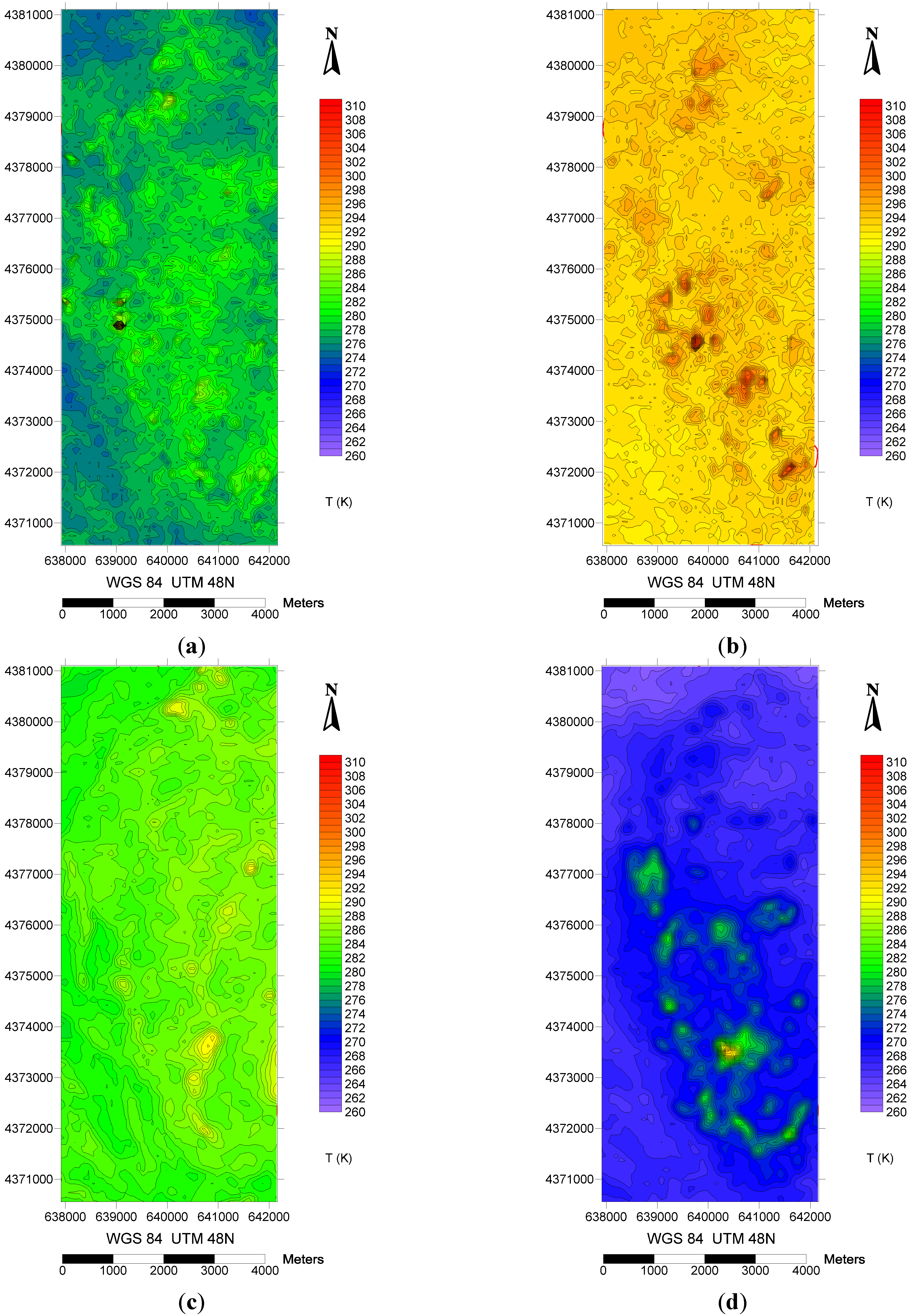
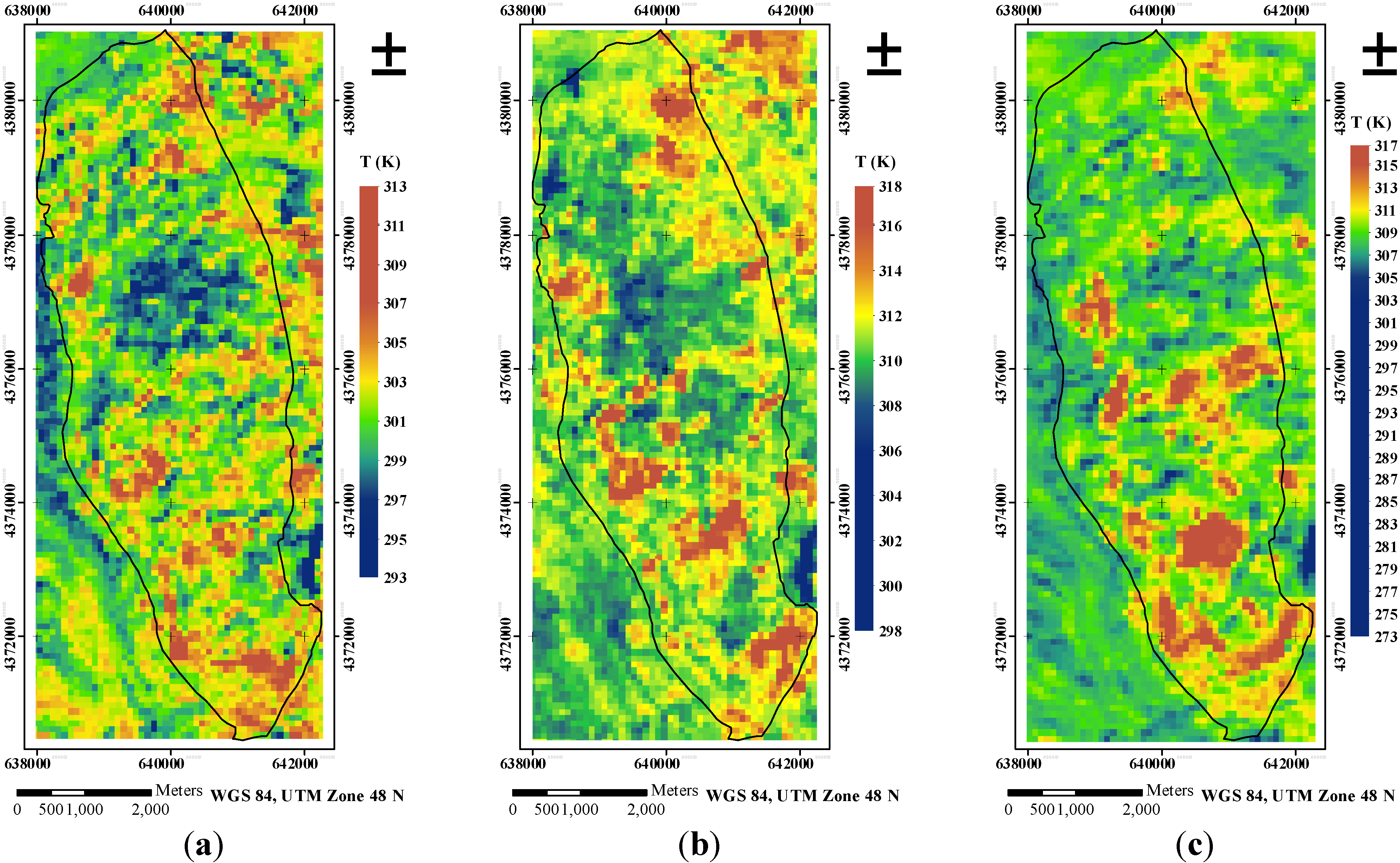
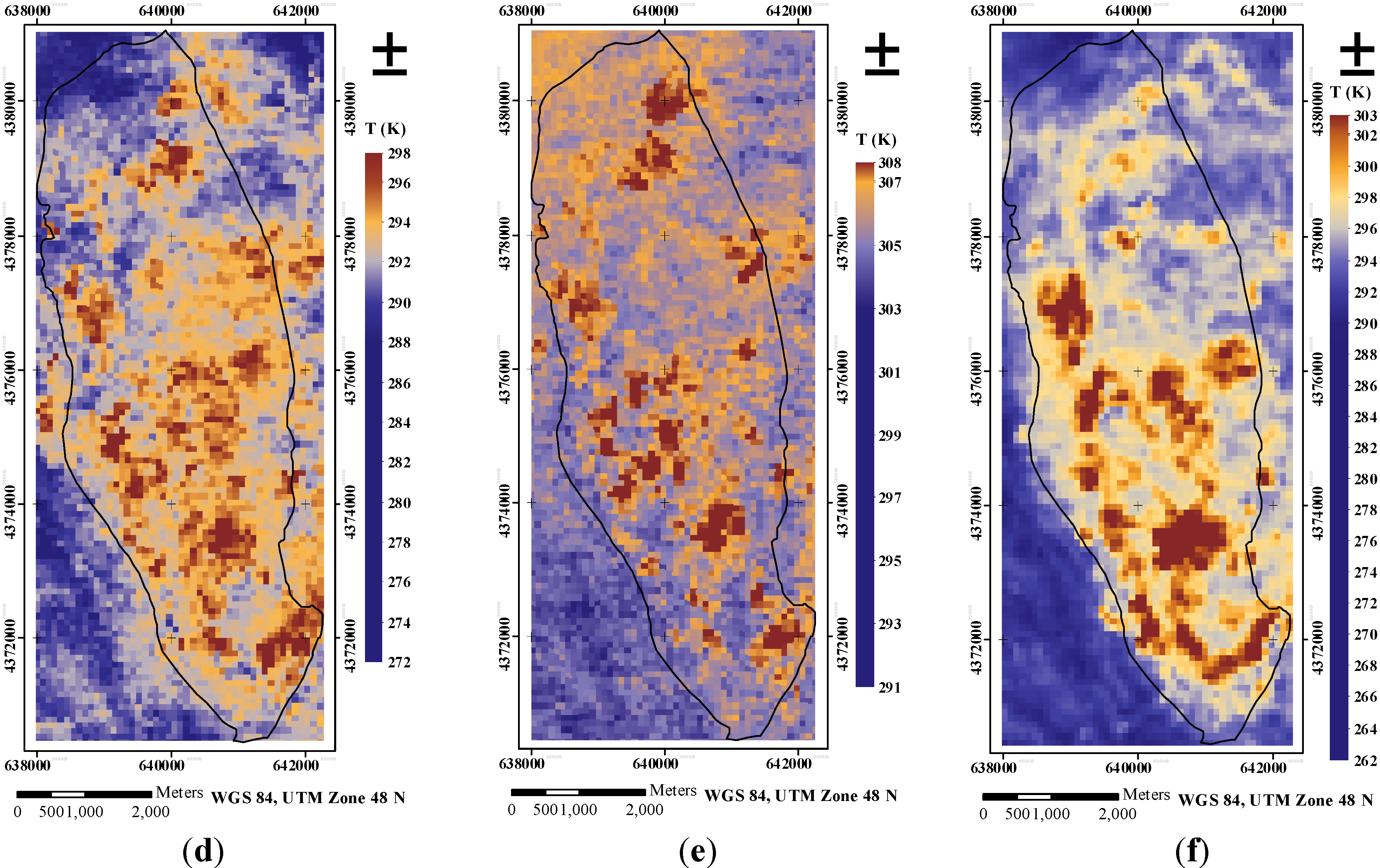
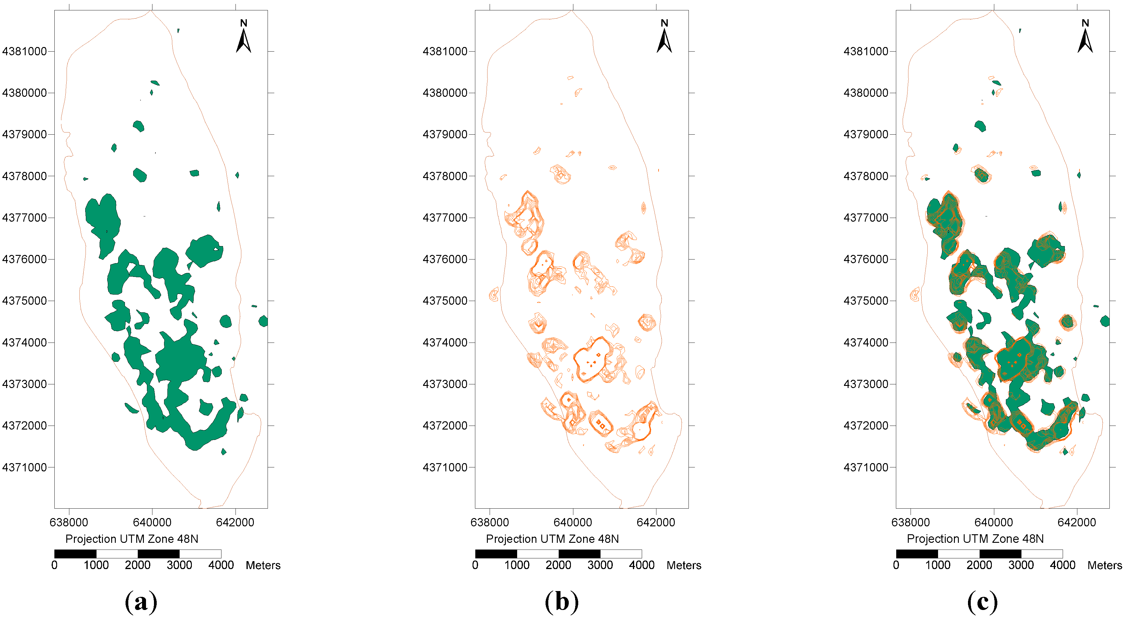
The analyses of images acquired during different seasons and image pairs acquired on the same date showed that the thermal anomalies present seasonal differences, but the day and night temperature distributions are similar. We observed an attenuation of the coal fire’s temperature on the edges of the coal fire’s boundaries, which resulted in extremely high gradient values along the boundaries. Based on this characteristic, we implemented a gradient-based thresholding method with the following three modules: gradient, temperature, and threshold definition. The image analysis incorporated an extended Sobel filter to process the supersampled TIR images and generate a regional temperature gradient representation. In addition, we used mathematical morphology thinning to skeletonize a potential high gradient buffer image and match the high temperature buffers to estimate the threshold. Better results were achieved using the mean threshold derived from the multiple potential high gradient buffers.

Methods based on ASTER images can effectively detect thermal anomalies. We delineated the anomalies using a TES-MMD method without emissivity and meteorological data. The SAGBT method is remote sensing-based; it primarily depends on the most direct coal fire-induced factor and energy release and uses the basic outer boundaries of the coal-bearing stratum to simply exclude false alarms. The proposed gradient-based thresholding method is a spatially based method to retrieve thermal anomalies from the different images obtained during the nighttime and daytime. This method is non-interactive and programmed by the IDL and primarily relies on the images’ thermal distributions. This method used a limited and basic field/geological dataset; it is a relatively simple and economical method to estimate the intensity of regional coal fires. It also presents an opportunity to detect long-term coal fire changes using the ASTER TIR images from the historical inventory. In addition, this method offers an alternative way to detect unknown coal fires in a certain area without sufficient in situ observations and field surveying data.

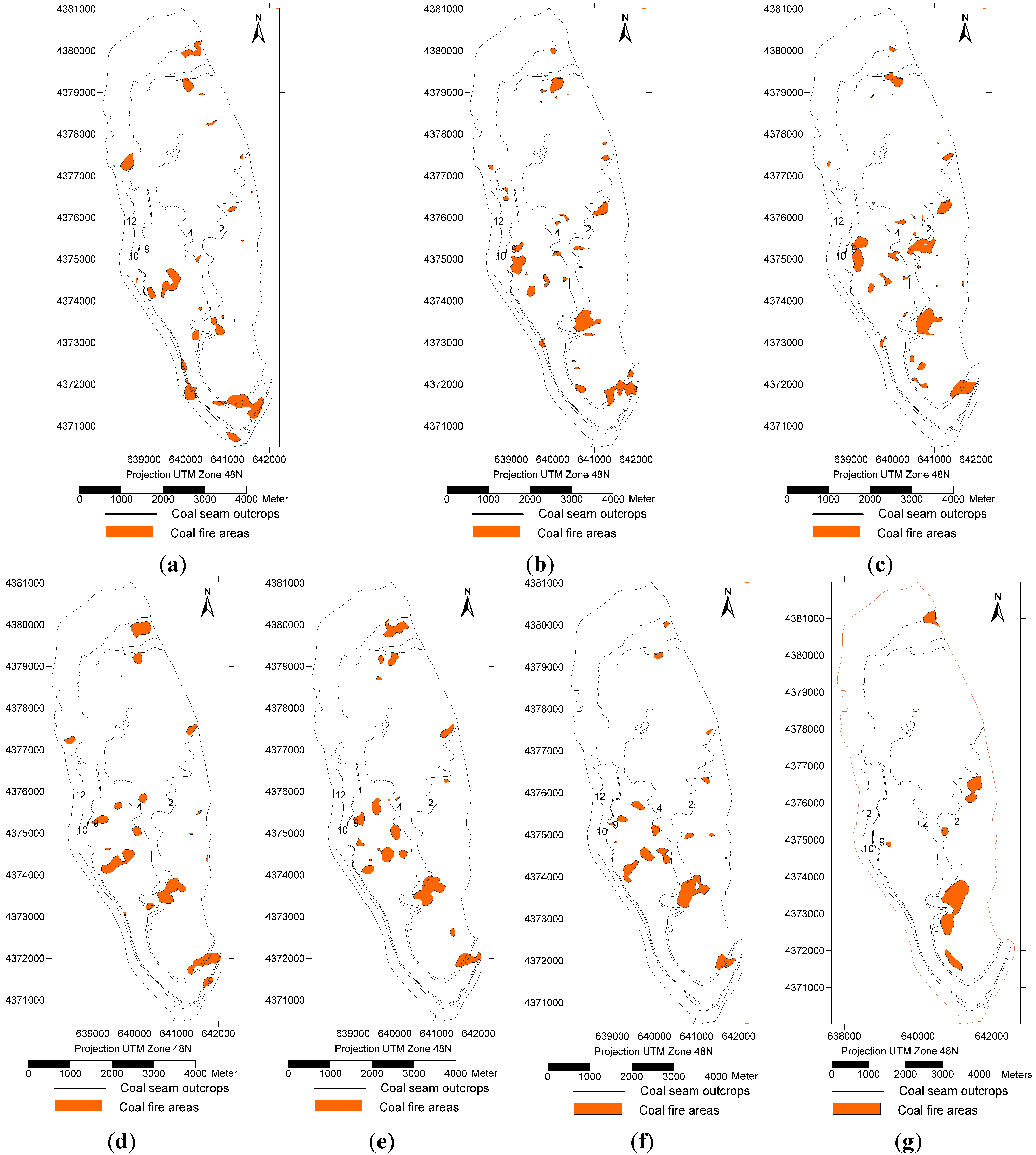
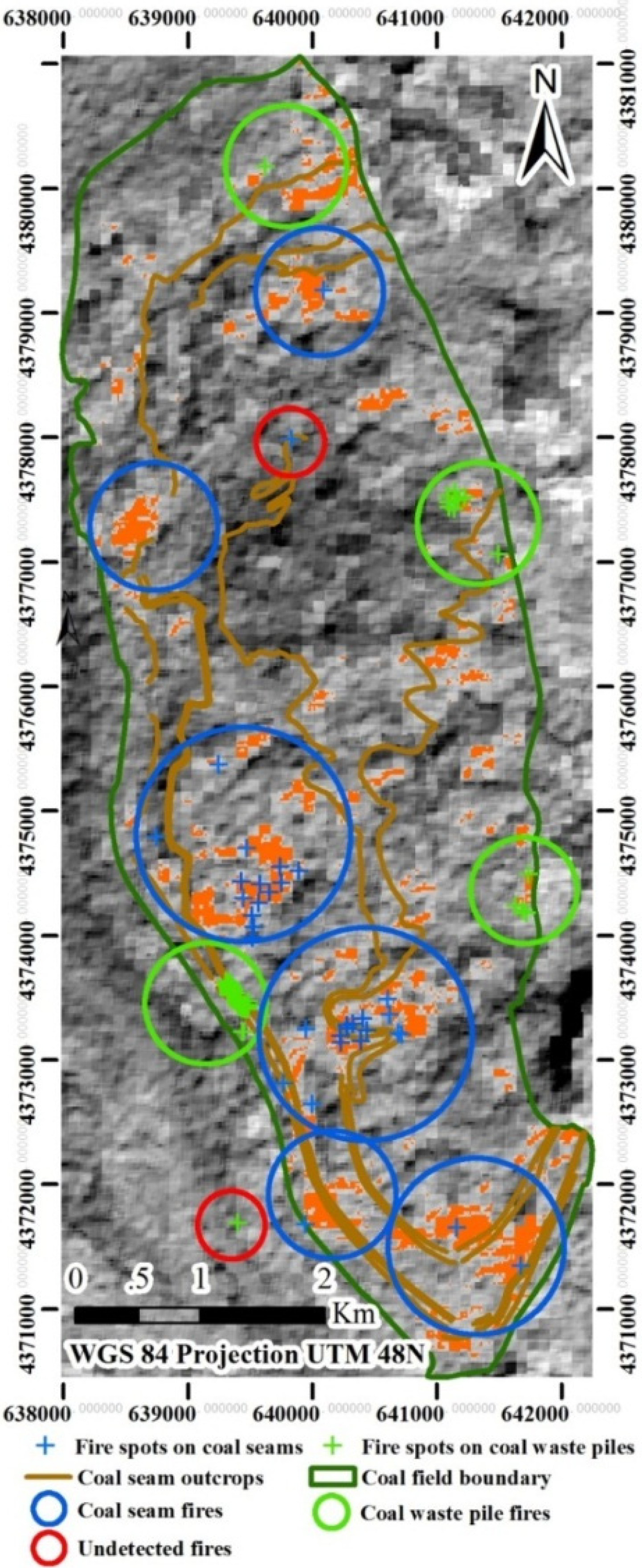
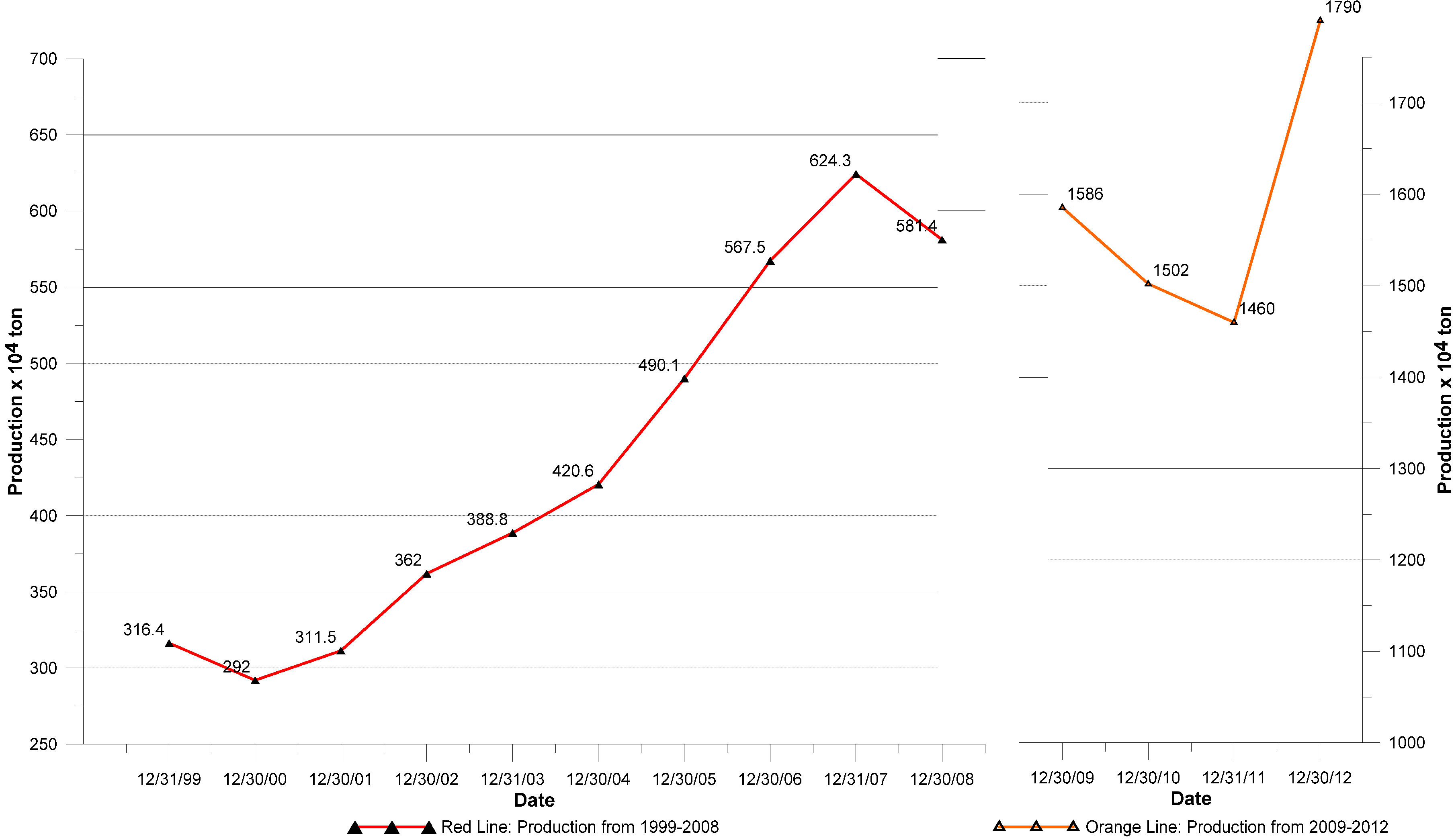
Fire maps show that fire areas are located along the coal seam outcrops, particularly the coal seam numbers 2, 4, and 9. The change detection time series plot reveals that, during the initial years, the fire areas started to decrease but soon began to increase moderately from 2003 to 2007. Since 2008, the spread of fires has sharply decreased, which was most likely because of government-sponsored extinguishing efforts. However, the spread of fires sharply increased again after 2010. With the comparison of the historical industrial figures, we found that the fluctuation of coal fire areas is similar to the curve of coal production in the Wuda Coalfield. Meanwhile, the coal fire area also shows a positive correlation with coal productivity in China, supported by the coal production over the last decade. We infer that coal fires are related to human activities, particularly mining. Additionally, the CO₂ emissions in the study period (2001–2010) were estimated to be 71.16 × 10⁴ tons.

Using the calibrated SAGBT method and the MMD-TES algorithm, we offer a novel approach to delineate coal fires in northern China and other coal fires that exist in the country using the historical inventory of TIR data without ground measurements and meteorological records. This non-interactive SAGBT method also offers the possibility to create multi-temporal change products using a uniform criterion for the temperature anomalies i.e., coal fires. These products will aid investigation of the resources lost, the environmental impacts, and the greenhouse gas emissions from coal seam combustion in the long term.

However, coal fires are complex from a remote sensing perspective and are difficult to accurately detect. This study focused on a subset of the Wuda syncline, and the geological and land cover/use in this area is relative homogeneous. Thus, if we extend the SAGBT method to other large-scale coal fire areas, then this method must be improved in the following ways: partition by the geological setting, geomorphology and land cover/use, so that the SAGBT method can be used in each small regional area; and study more specific false alarm removal criteria to exclude false alarms (such as water bodies, illuminated slopes, and industrial plants) or map a fire risk area to mask coal fire-related anomalies. In particular, emissivity data are very useful in identifying geological boundaries such as strata boundaries and faults, which could help to divide a large area. When improved, emissivity anomalies could be considered as a data source to determine coal fires or eliminate false fires. We observed that removing solar irradiation can improve the accuracy of coal fire detection for daytime TIR images. In this work, due to the reduced vegetation coverage in the Wuda Coalfield and even in Northwestern China, coal fires are less often confused with wild fires. However, separating coal fires from wild fires is essential in order to extend the SAGBT worldwide. A combination of coal fire risk area, coal fire-induced surface characteristics, and very high temperature areas were expected to be modeled as accepting/rejecting criteria for distinguishing coal fires from wild fires. Further research should also focus on using field survey data collected on the ASTER overpass date and the estimation of the ASTER sensor’s degradation effects on the detection of anomalies.

Acknowledgments

Funding for this work was provided by a Strategic Priority Research Program of the Chinese Academy of Sciences, Carbon Emission from Coal Spontaneous Combustion (Grant No. XDA05030200). The first author’s visiting study at the University of Georgia (UGA) was sponsored by the China Scholarship Council. We thank Guang Yang and Zhipeng Li for collection of field data. The authors wish to thank the anonymous reviewers for their constructive suggestions that improved the paper. Image acquisition was granted by the Land Processes Distributed Active Archive Center (LP DAAC) of the National Aeronautics and Space Administration (NASA), including the tasking of the ASTER orbital sensor to acquire images during field activities in China. ASTER images were accessed through the Earth Resources Observation Systems (EROS) Data Center of the U.S. Geological Survey (USGS). Special thanks to UGA’s international student internship program for facilitating collaboration between the two institutes.

Author Contributions

Xiaomin Du, Deepak Mishra, and Sergio Bernardes, designed the research, programmed software, defined image processing and data analysis approaches, processed images, analyzed data, interpreted results, and wrote the manuscript. Daiyong Cao managed the coal fire detection project, offered professional consultation in coal fire detection methods, contributed valuable coal fire documents and data, planned the field surveying and provided the logistical support. Thomas R. Jordan scheduled image acquisition and planned the field surveying. Marguerite Madden supported the interpretation of the change detection, and the writing and editing of the manuscript.

Conflicts of Interest

The authors declare no conflict of interest.

References

Prakash, A.; Schaefer, K.; Witte, W.K.; Collins, K.; Gens, R.; Goyette, M.P. A remote sensing and GIS based investigation of a boreal forest coal fire. Int. J. Coal Geol. 2011, 86, 79–86. [Google Scholar] [CrossRef]
Chatterjee, R.S. Coal fire mapping from satellite thermal IR data—A case example in Jharia Coalfield, Jharkhand, India. ISPRS J. Photogramm. Remote Sens. 2006, 60, 113–128. [Google Scholar] [CrossRef]
Pone, J.D.N.; Hein, K.A.; Stracher, G.B.; Annegarn, H.J.; Finkleman, R.B.; Blake, D.R.; McCormack, J.K.; Schroeder, P. The spontaneous combustion of coal and its by-products in the Witbank and Sasolburg coalfields of South Africa. Int. J. Coal Geol. 2007, 72, 124–140. [Google Scholar] [CrossRef]
Zhang, J. Underground Coal Fires in China: Origin, Detection, Fire-Fighting, and Prevention; China Coal Industry Publishing House: Beijing, China, 2008. [Google Scholar]
Jiang, L.; Lin, H.; Ma, J.; Kong, B.; Wang, Y. Potential of small-baseline SAR interferometry for monitoring land subsidence related to underground coal fires: Wuda (Northern China) case study. Remote Sens. Environ. 2011, 115, 257–268. [Google Scholar] [CrossRef]
Prakash, A. Coal fires—A Natural or Man Made Hazard? Available online: http://www2.gi.alaska.edu/~prakash/coalfires/coalfires.html (accessed on 20 May 2015).
van Dijk, P.; Zhang, J.; Jun, W.; Kuenzer, C.; Wolf, K.H. Assessment of the contribution of in-situ combustion of coal to greenhouse gas emission; based on a comparison of Chinese mining information to previous remote sensing estimates. Int. J. Coal Geol. 2011, 86, 108–119. [Google Scholar] [CrossRef]
Kuenzer, C.; Hecker, C.; Zhang, J.; Wessling, S.; Wagner, W. The potential of multidiurnal MODIS thermal band data for coal fire detection. Int. J. Remote Sens. 2008, 29, 923–944. [Google Scholar] [CrossRef]
Slavecki, R.J. Detection and location of subsurface coal fires. In Proceedings of the Third Symposium on Remote Sensing of Environment, Ann Arbor, MI, USA, 14–16 October, 1964; pp. 537–547.
Greene, G.W.; Moxham, R.M.; Harvey, A.H. Aerial infrared surveys and borehole temperature measurements of coal mine fires in Pennsylvania. Remote Sens. Environ. 1969, 1, 517–525. [Google Scholar]
Bhattacharya, A.; Reddy, S.; Mukherjee, T. Multi-tier remote sensing data analysis for coalfire mapping in Jharia Coalfield of Bihar, India. In Proceedings of the Twelfth Asian Conference on Remote Sensing, Singapore, 30 October–5 November 1991; pp. 21–22.
Cracknell, A.; Mansor, S. Detection off sub-surface coal fires using Landsat Thematic Mapper data. Int. Arch. Photogramm. Remote Sens. 1993, 29, 750–753. [Google Scholar]
Saraf, A.K.; Prakash, A.; Sengupta, S.; Gupta, R.P. Landsat TM data for estimating ground temperature and depth of subsurface coal fire in the Jharia Coalfield, India. Int. J. Remote Sens. 1995, 16, 2111–2124. [Google Scholar] [CrossRef]
Prakash, A.; Gupta, R. Surface fires in Jharia coalfield, India-their distribution and estimation of area and temperature from TM data. Int. J. Remote Sens. 1999, 20, 1935–1946. [Google Scholar] [CrossRef]
Gangopadhyay, P.K.; Maathuis, B.; Van Dijk, P. ASTER-derived emissivity and coal-fire related surface temperature anomaly: A case study in Wuda, North China. Int. J. Remote Sens. 2005, 26, 5555–5571. [Google Scholar] [CrossRef]
Jiang, W.; Gu, L.; Yang, B.; Chen, Q. Monitoring method of underground coal fire based on night thermal infrared remote sensing technology. Spectrosc. Spectral Anal. 2011, 31, 357–361. [Google Scholar]
Tetzlaff, A. Coal Fire Quantification using ASTER, ETM and BIRD Satellite Instrument Data. Ph.D. Thesis, Ludwig-Maximilians-Universität München (LMU), Munich, Germany, 2004. [Google Scholar]
Chen, Y.; Jing, L.; Bo, Y.; Shi, P.; Zhang, S. Detection of coal fire location and change based on multi‐temporal thermal remotely sensed data and field measurements. Int. J. Remote Sens. 2007, 28, 3173–3179. [Google Scholar] [CrossRef]
Prakash, A.; Gupta, R.; Saraf, A. A Landsat TM based comparative study of surface and subsurface fires in the Jharia Coalfield, India. Int. J. Remote Sens. 1997, 18, 2463–2469. [Google Scholar] [CrossRef]
Zhang, X.; Cassells, C.; Van Genderen, J. Multi-sensor data fusion for the detection of underground coal fires. Geol. Mijnb. 1998, 77, 117–128. [Google Scholar] [CrossRef]
Yang, B.; Chen, Y.; Li, J.; Gong, A.; Kuenzer, C.; Zhang, J. Simple normalization of multi-temporal thermal IR data and applied research, on the monitoring of typical coal fires in northern China. In Proceedings of the 2005 IEEE International Geoscience and Remote Sensing Symposium Proceedings(25th) (IGARSS 2005), Seoul, Korea, 25–29 July 2005; pp. 5725–5728.
Dozier, J. A method for satellite identification of surface temperature fields of subpixel resolution. Remote Sens. Environ. 1981, 11, 221–229. [Google Scholar] [CrossRef]
Voigt, S.; Tetzlaff, A.; Zhang, J.; Künzer, C.; Zhukov, B.; Strunz, G.; Oertel, D.; Roth, A.; van Dijk, P.; Mehl, H. Integrating satellite remote sensing techniques for detection and analysis of uncontrolled coal seam fires in North China. Int. J. Coal Geol. 2004, 59, 121–136. [Google Scholar] [CrossRef]
Kuenzer, C.; Zhang, J.; Li, J.; Voigt, S.; Mehl, H.; Wagner, W. Detecting unknown coal fires: Synergy of automated coal fire risk area delineation and improved thermal anomaly extraction. Int. J. Remote Sens. 2007, 28, 4561–4585. [Google Scholar] [CrossRef]
Zhang, J. Spatial and Statistical Analysis of Thermal Satellite Imagery for Extraction of Coal Fire Related Anomalies. Ph.D. Thesis, Technical University Vienna, Vienna, Austria, 2004. [Google Scholar]
Lasaponara, R.; Cuomo, V.; Macchiato, M.; Simoniello, T. A self-adaptive algorithm based on AVHRR multitemporal data analysis for small active fire detection. Int. J. Remote Sens. 2003, 24, 1723–1749. [Google Scholar] [CrossRef]
Kuenzer, C.; Zhang, J.; Hirner, A.; Bo, Y.; Jia, Y.; Sun, Y. Multitemporal in-situ mapping of the Wuda coal fires from 2000 to 2005-assessing coal fire dynamics. In Spontaneous Coal Seam Fires: Mitigating a Global Disaster; UNESCO: Beijing, China, 2008; ERSEC ecological book serie 4; pp. 132–148. [Google Scholar]
Kuenzer, C.; Zhang, J.; Tetzlaff, A.; Voigt, S.; Wagner, W. Automated demarcation, detection and quantification of coal fires in China using remote sensing data. In Spontaneous Coal Seam Fires: Mitigating a Global Disaster; Tsinghua University Press: Beijing, China, 2008; pp. 362–380. [Google Scholar]
Kuenzer, C.; Zhang, J.; Sun, Y.; Jia, Y.; Dech, S. Coal fires revisited: The Wuda coal field in the aftermath of extensive coal fire research and accelerating extinguishing activities. Int. J. Coal Geol. 2012, 102, 75–86. [Google Scholar] [CrossRef]
Guney, M. Oxidation and spontaneous combustion of coal: review of individual factors. Colliery Guard. 1968, 216, 105–110. [Google Scholar]
Cao, D.; Fan, X.; Guan, H.; Wu, C.; Shi, X.; Jia, Y. Geological models of spontaneous combustion in the Wuda Coalfield, Inner Mongolia, China. Rev. Eng. Geol. 2007, 18, 23–30. [Google Scholar]
Zhang, J.; Kuenzer, C. Thermal surface characteristics of coal fires 1 results of in-situ measurements. J. Appl. Geophys. 2007, 3, 117–134. [Google Scholar] [CrossRef]
Kuenzer, C.; Strunz, G.; Voigt, S.; Wagner, W. Multitemporal landcover investigations in a semi-arid mining environment: Coal fire areas in Northern China. In Proceedings of the Conference of the EARSeL Special Interest Group on Land Use and Land Cover, Dubrovnik, Croatia, 25–27 May 2004; pp. 47–57.
Li, J.; Voight, S.; Kunzer, C.; Yang, B.; Zhang, J.; Zhang, Y.; Kong, B.; Zhange, S. The progress in detecting of coal fire on remote sensing the first result of the joint Sino-German research project on innovative technologies for exploration, extinction and monitoring of coal fires in North China. In Proceedings of the 2005 Dragon Symposium “Mid-Term Results”, Santorini, Greece, 27 June–1 July 2005; Volume 27.
Yang, B.; Chen, Y.; Li, J.; Gong, A.; Kuenzer, C.; Zhang, J. Simple Normalization of Multi-temporal Thermal IR Data and Applied Research on the Monitoring of Typical Coal Fires in Northern China; Beijing Normal University: Beijing, China, 2005. [Google Scholar]
Chen, Y.; Jing, L.; Bo, Y.; Shi, P.; Zhang, S. Detection of coal fire location and change based on multi-temporal thermal remotely sensed data and field measurements. Int. J. Remote Sens. 2007, 28, 3173–3179. [Google Scholar] [CrossRef]
Jiang, W.; Wu, J.; Gu, L.; Liu, X.; Li, X. Change monitoring in Wuda Coalfield fire area based on remote sensing. J. China Coal Soc. 2010, 35, 964–968. (In Chinese) [Google Scholar]
Peng, S.; Zhang, J. Coal Bearing Strata Sedimentary Environment and its Influence in the Wuda Coal Mining Area; Mining Coal Industry Publishing House: Beijing, China, 1995. (In Chinese) [Google Scholar]
Yu, Z.; Li, F.; Tian, F.; Sun, T.; Du, X. The influence of NDVI for land surface temperature retrieval from Landsat 5 in the Wuda District, China. In Proceedings of the 2012 Second International Conference on Electric Information and Control Engineering (ICEICE), Lushan, China, 6–8 April 2012; Volume 7, pp. 5396–5404.
China Coal Information Research Institute, State Administration of Coal Mine Safety. China Coal Industry Yearbook (2001–2011); China Coal Industry Publishing House: Beijing, China, 2002–2012. (In Chinese) SACMS (2001 to 2011) [Google Scholar]
Zhang, Y.; Shi, W. Shenhua Wuhai Energy: Mortality Rate Per Million Tons Declined to Zero. Inner Mongolia Daily for 5 January 2013, the Third Page. Available online: http://szb.northnews.cn/nmgrb/page/52/2013-01-05/03/57071357354841420.pdf (accessed on 20 May 2015). (In Chinese)
Young, S.J.; Johnson, B.R.; Hackwell, J.A. An in-scene method for atmospheric compensation of thermal hyperspectral data. J. Geophys. Res.: Atmos. 2002, 107. [Google Scholar] [CrossRef]
DiStasio, R.J., Jr.; Resmini, R.G. Atmospheric compensation of thermal infrared hyperspectral imagery with the emissive empirical line method and the in-scene atmospheric compensation algorithms: A comparison. In Proceedings Algorithms and technologies for multispectral, hyperspectral, and ultraspectral imagery XVI, Orlando, Florida, USA, 12 May 2010.
Sobrino, J.A.; Li, Z.L.; Soria, G.; Jiménez, J.C. Land surface temperature and emissivity retrieval from remote sensing data. Recent Res. Dev. Geophys. 2002, 4, 21–44. [Google Scholar]
Dash, P.; Göttsche, F.-M.; Olesen, F.-S.; Fischer, H. Land surface temperature and emissivity estimation from passive sensor data: Theory and practice-current trends. Int. J. Remote Sens. 2002, 23, 2563–2594. [Google Scholar] [CrossRef]
Kerr, Y.H.; Lagouarde, J.P.; Nerry, F.; Ottlé, C. Land surface temperature retrieval techniques and applications. In Thermal remote sensing in land surface processes; CRC Press: Boston, MA, USA, 2004; pp. 33–109. [Google Scholar]
Ottlé, C.; Vidal-Madjar, D. Estimation of land surface temperature with NOAA9 data. Remote Sens. Environ. 1992, 40, 27–41. [Google Scholar] [CrossRef]
Prata, A.J. Land surface temperatures derived from the advanced very high resolution radiometer and the along-track scanning radiometer: 1. Theory. J. Geophys. Res.: Atmos. 1993, 98, 16689–16702. [Google Scholar] [CrossRef]
Sobrino, J.A.; Cuenca, J. Angular variation of thermal infrared emissivity for some natural surfaces from experimental measurements. Appl. Opt. 1999, 38, 3931–3936. [Google Scholar] [CrossRef] [PubMed]
Kahle, A.B.; Madura, D.P.; Soha, J.M. Middle infrared multispectral aircraft scanner data: Analysis for geological applications. Appl. Opt. 1980, 19, 2279–2290. [Google Scholar] [CrossRef] [PubMed]
Gillespie, A.R. Lithologic mapping of silicate rocks using TIMS. In Proceedings of the Thermal Infrared Multispectral Scanner (TIMS) Data Users' Workshop, Pasadena, CA, USA, 1 November 1986; pp. 29–44.
Kealy, P.S.; Gabell, A.R. Estimation of emissivity and temperature using alpha coefficients. In Proceedings of the 2nd Thermal Infrared Multispectral Scanner (TIMS) Workshop, Pasadena, CA, USA, 6 June 1990; pp. 11–15.
Becker, F.; Li, Z.L. Temperature-independent spectral indices in thermal infrared bands. Remote Sens. Environ. 1990, 32, 17–33. [Google Scholar] [CrossRef]
Watson, K. Spectral ratio method for measuring emissivity. Remote Sens. Environ. 1992, 42, 113–116. [Google Scholar] [CrossRef]
Gillespie, A.; Rokugawa, S.; Matsunaga, T.; Cothern, J.S.; Hook, S.; Kahle, A.B. A temperature and emissivity separation algorithm for advanced spaceborne thermal emission and reflection radiometer (aster) images. IEEE Trans. Geosci. Remote Sens. 1998, 36, 1113–1126. [Google Scholar] [CrossRef]
Soille, P. Morphological Image Analysis: Principles and Applications; Springer-Verlag Inc.: New York, NY, USA, 2003. [Google Scholar]
Thinning. Available online: http://homepages.inf.ed.ac.uk/rbf/HIPR2/thin.htm (accessed on 20 May 2015).
Wessling, S.; Kuenzer, C.; Kessels, W.; Wuttke, M.W. Numerical modeling for analyzing thermal surface anomalies induced by underground coal fires. Int. J. Coal Geol. 2008, 74, 175–184. [Google Scholar] [CrossRef]
Du, X.; Cao, D.; Yang, G. Estimating typical four-season thermal distribution and self-adaptive gradient based thresholding parameters over coal fire areas in China using ASTERand LDCM TIRS-a case study in the Wuda Coalfield, China. In Proceeding of the ASPRS 2014 Conferennce, Louisville, KY, USA, 23–28 March 2014.
Kong, B.; Ma, J.; Chen, H.; Zhang, X. The application of 3S technology to assessment of the flood risk in the Wuda Coal Mine, Inner Mongolia. Remote Sens. Land Resour. 2010, 2, 80–85. (In Chinese) [Google Scholar]
Du, X.; Peng, S.; Wang, H.; Bernardes, S.; Yang, G.; Li, Z. Annual change detection by ASTER TIR data and an estimation of the annual coal loss and CO₂ emission from coal seams spontaneous combustion. Remote Sens. 2015, 7, 319–341. [Google Scholar] [CrossRef]

© 2015 by the authors; licensee MDPI, Basel, Switzerland. This article is an open access article distributed under the terms and conditions of the Creative Commons Attribution license (http://creativecommons.org/licenses/by/4.0/).

Share and Cite

MDPI and ACS Style

Du, X.; Cao, D.; Mishra, D.; Bernardes, S.; Jordan, T.R.; Madden, M. Self-Adaptive Gradient-Based Thresholding Method for Coal Fire Detection Using ASTER Thermal Infrared Data, Part I: Methodology and Decadal Change Detection. Remote Sens. 2015, 7, 6576-6610. https://doi.org/10.3390/rs70606576

AMA Style

Du X, Cao D, Mishra D, Bernardes S, Jordan TR, Madden M. Self-Adaptive Gradient-Based Thresholding Method for Coal Fire Detection Using ASTER Thermal Infrared Data, Part I: Methodology and Decadal Change Detection. Remote Sensing. 2015; 7(6):6576-6610. https://doi.org/10.3390/rs70606576

Chicago/Turabian Style

Du, Xiaomin, Daiyong Cao, Deepak Mishra, Sergio Bernardes, Thomas R. Jordan, and Marguerite Madden. 2015. "Self-Adaptive Gradient-Based Thresholding Method for Coal Fire Detection Using ASTER Thermal Infrared Data, Part I: Methodology and Decadal Change Detection" Remote Sensing 7, no. 6: 6576-6610. https://doi.org/10.3390/rs70606576

Article Menu

Self-Adaptive Gradient-Based Thresholding Method for Coal Fire Detection Using ASTER Thermal Infrared Data, Part I: Methodology and Decadal Change Detection

Abstract

1. Introduction

2. Study Area and Data

2.1. Study Regions

2.2. Remote Sensing Data for Algorithm Development

2.3. Remote Sensing Data for Decadal Change Detection (2001 to 2011)

2.4. Coal Production Data for the Wuda Coalfield

3. Preliminary Data Preprocessing and Analysis

3.1. Atmospheric Correction

3.2. Land Surface Temperature and Land Surface Emissivity Retrieval

3.3. Reasons for Gradient-Based Thresholding: Seasonal and Diurnal Variations in the Thermal Distribution

3.4. Thermal Anomalies and the Definition of Coal Fire Areas

4. Algorithm of SAGBT

4.1. The Workflow of SAGBT

4.2. Gradient Calculation

4.3. Potential High Gradient Buffers

4.4. High Temperature Buffers

4.5. Mathematical Morphology Thinning and Extremely High Gradient Lines

4.6. Fine-Tuning Threshold and Thermal Anomalies

5. Performance of SAGBT

5.1. Convergence Analysis

5.2. Coal Fire Mapping and Comparisons

5.3. Uncertainty and Accuracy

6. Application of SAGBT on Decadal Change Detection

6.1. Changes and Time Series Analysis

6.2. Comparison of Coal Fire Areas and Coal Production over the Ten-Year Period

7. Conclusions and Vision

Acknowledgments

Author Contributions

Conflicts of Interest

References

Share and Cite

Article Metrics

Article Access Statistics

Further Information

Guidelines

MDPI Initiatives

Follow MDPI