1. Introduction
Wetlands are important for the ecosystem services they provide, including flood mitigation, water purification, wildlife habitat and recreational potential [
1,
2]. Wetlands can be highly dynamic, particularly with regard to inundation, and this dynamism has important implications for carbon and methane cycling [
3]. The value of wetlands is evidenced by multiagency and non-government collaborative efforts to restore and preserve them. In the case of the Everglades of South Florida, USA, a multi-decade, multi-billion dollar effort to restore flow characteristics, and therefore habitat conditions and fauna health, has been underway [
4]. For Everglades restoration science to be most efficient and effective, scientists and managers need information on surface water extent, depth and hydroperiod, that is, the length of time or portion(s) of the year a wetland holds ponded water.
The Everglades Depth Estimation Network (EDEN) was developed as a set of tools to model surface water dynamics and guide field and other types of Everglades studies [
5]. The EDEN is an information and applications system that provides hydrologic and ecologic modelers as well as field scientists and resource managers with spatially distributed, daily information on water depth, precipitation and evapotranspiration. Based on a region-wide geospatial framework [
6], the EDEN is a compilation of an extensive gage network managed by numerous agencies, surface water heights modeled from those gages [
7] and digital elevation models (DEMs) derived from thousands of sub-water surface ground height measurements [
8]. This may be the most extensive wetland gage network in the world and is certainly a unique dataset for a variety of hydrologic, biologic and remote sensing experiments. The resolution of the EDEN grid (500 m) is finer than the 2 mile by 2 mile model used to simulate the entire region [
9]. However, research on the scale lengths over which Everglades vegetation varies [
10,
11] indicates that finer spatial resolution would better represent Everglades vegetation patterns, and by extension, the elevation and inundation dynamics that shape them. Useful information on inundation derived from Landsat would complement EDEN through the provision of higher spatial resolution, longer-term records of Everglades surface water dynamics than can be realized through EDEN alone.
The Everglades subtropical climate and dynamic land (water) cover present great challenges for remote sensing [
12,
13]. While active systems such as radar allow for cloud penetration, the detection of Everglades surface inundation or hydroperiods [
14,
15] and changes in water levels [
16,
17,
18], radar archives are not available with either the temporal frequency or multi-decadal observations afforded by the Landsat Archive. Frequent, extensive cloud cover had made the use of optical remote sensing at even low temporal frequency cost prohibitive in the past. However, release of Landsat data at no cost to the user presents an opportunity to economically investigate whether Landsat data might be used to characterize Everglades (and other wetland) dynamics at spatial resolutions and for a sufficient length of time as to inform Everglades studies and finer resolution hydrologic/ecologic modeling [
13].
The USGS is developing Climate Data Records and other Landsat Science Products from data collected by Landsats 4 through 8 with the intention of distributing these products to the public at no cost to the user. One such product is named “Dynamic Surface Water Extent” (DSWE) [
19]. While the developed approach might be applied to any scene in the archive, the expressed goal of DSWE development is the detection of surface water extent in any cloud/shadow/snow free pixel in the Landsat Archive for the United States and its territories. This requires appropriate characterization of the uncertainty associated with dynamic surface water mapping in the United States.
The concept of mapping surface water using Landsat is by no means novel. Techniques applied range in complexity and general applicability. Some simply use thresholds on individual Landsat bands [
20,
21] or band ratios [
21,
22,
23,
24,
25,
26,
27,
28]. A threshold-based method specifically designed for areas of complex, shadowy terrain [
29] exhibits higher accuracy than band ratio based techniques. While proposed thresholds are relatively stable, they still require modification for areas or places beyond those for which they were developed. Other research has applied parametric [
30] or non-parametric classification techniques, such as classification and regression trees (CART) [
31,
32]. Although currently favored given their ability to use multi-scalar input data (such as thematic ancillary information), CART models require significant amounts of training data for calibration and validation. Object-based image analysis (OBIA) has been applied using Landsat to identify wetlands in a region of Florida well north of the Everglades [
33]. Unlike the Everglades, the open water areas of those wetlands are relatively large, with well-defined boundaries compared to the highly mixed and dynamic Everglades system. A review of the growing literature regarding the application of OBIA to wetlands mapping [
34] concluded that the capacity to use OBIA to monitor wetland dynamics lags behind static wetland identification and highlighted OBIA complexities that make standardized application of OBIA to wetland monitoring challenging. Since OBIA is relatively processing intensive, it would be costly to apply to every scene in the Landsat Archive. Subpixel classification via spectral unmixing [
35,
36], regression trees [
32,
37] and other analytical methods [
38] have also been employed. Authors have used these various techniques in combination, such as OBIA with thresholds on individual bands and (or) band ratios [
25]. Previous efforts to specifically map Everglades inundation via optical satellite sensors [
39,
40,
41] suggest that optical satellite data could be useful. However, all three studies were limited in spatial and temporal scope. That is, each evaluated a particular subarea of the Greater Everglades for a one year period or less. The methods used for each study required extensive training, subjective interaction through multi-stage classification or the use of gage data for both algorithm development and assessment. Finally, all references reviewed alluded to the influence of vegetation cover in reducing accuracy without explicitly addressing the issue.
1.1. Goal and Objectives
The primary goal of this research was to assess the efficacy of a proposed inundation algorithm that applies static thresholds to surface reflectance calibrated Landsat data–in essence a “training free” method of detecting inundated areas in a marshland dominated environment. Three objectives were pursued to achieve this goal: (1) Develop an approach using the EDEN gage data to evaluate satellite derived surface water extent products for vegetation covered, inundated areas; (2) Use this approach to assess a prototype DSWE algorithm’s performance in an objective and informative manner, and (3) Examine how well a single algorithm applied to multiple scenes without training data affords monitoring of surface water extent at high spatial resolution in wetland environments like the Everglades.
1.2. Expectations and Caveats on Model Performance
Given some understanding of wetland environments that are vegetation-covered and only periodically flooded, a conceptual model regarding the spatial and temporal variations in model performance might be formulated a priori. For example, poorest performance might be expected in locations of thick vegetation canopy where omission errors should be high. In turn, this expectation might lead to the conclusion that the model will “perform best” during periods of low water levels, when water is near or below the ground surface. At these times, areas with dense vegetation, due to higher elevation, dry first, and the model’s inability to sense ground conditions under dense vegetation would result in a higher percentage of “correct answers” for the wrong reason. Also, one might expect poorer algorithm performance under hazy and (or) cloudy conditions. However, for the Everglades cloudy conditions are also most prevalent during the high water or wet season. Would this reduce model effectiveness under wet conditions as well? Finally, atmospheric effects on model performance might be particularly acute due to the reliance of the model on a physically-based decision rule that requires atmospheric correction under the most challenging conditions. The in situ data, knowledge of study area characteristics, and experimental design all employed here allow for empirical examination of these expectations.
2. Methods
2.1. Study Area
The Florida Everglades region of South Florida (
Figure 1), is a unique and important wetland ecosystem that historically stretched from the southern rim of Lake Okeechobee (the second largest freshwater lake in the United States) to Florida Bay [
42]. Currently bounded by agricultural and urban areas on its northern and eastern borders, it is composed of a system of large water impoundments (Water Conservation Areas, or WCAs) largely separated from one another by levees, canals and other water control structures that move water in and out of the WCAs to protect adjacent developed areas from flooding, as well as store and regulate water release in times of drought [
13]. The Everglades National Park (ENP) and the Big Cypress Nature Preserve (BCNP) cover the remainder of South Florida’s undeveloped mainland from north of the Tamiami Trail to the Florida Bay.
The Everglades is an extremely low gradient environment [
8] with an elevation range of approximately 5 m from the highest to lowest points that are more than 150 km apart (
Figure 1). Land cover within the wetlands is composed of mosaics of open water and wet prairie as well as herbaceous, shrub and forested wetlands [
43]. A majority of the Everglades area is covered by wet prairie and sawgrass marsh [
10], and it has long been referred to as the “river of grass” [
44].
Figure 1.
The Greater Everglades region of South Florida, USA. The digital elevation model covering the EDEN model domain, shows elevation in meters above sea level [
8] and illustrates the extremely flat nature of the Everglades. Subtle differences in topography create variations in hydroperiod that dictate vegetation composition. Reliable information on inundation dynamics would be very beneficial to restoration science and resource management. Non-tidally influenced areas of Water Conservation Areas (WCA) 1–3 are labelled simply as 1, 2A, 2B, 3AN, 3AS, and 3B.
With an average annual mean temperature of 25° C, southern Florida’s climate is classified as maritime subtropical, with long, hot summers (typically May through November) and mild, dry winters (approximately December through April) [
45,
46]. Annually, Florida receives 140 cm of rainfall [
47]. Depending on location, measured evaporation from periodically dry to permanently wet surfaces ranges from 50% to 110% of the annual precipitation average [
48]. Very low Everglades surface water flow velocities contribute to this evaporation, with relatively open flow features such as sloughs having recorded velocities ranging from up to 2 cm/s to less than 0.1 cm/s during the wet and dry seasons, respectively [
49]. Detailed water balance studies suggest that such high rates of evaporation and reduced flows to the ENP are creating increased saltwater influxes that are altering vegetation. An example is the landward migration of mangrove [
50]. Because water flow management to manipulate vegetation composition is viewed as one restoration mechanism [
4], high resolution data on inundation would be information used for restoration monitoring and adaptation [
12].
2.2. Satellite-Based Input Data
Provisional level 1T (terrain corrected) Landsat 5 Surface Reflectance, Landsat Climate Data Record (CDR) data, here abbreviated as “L5LSRP”, were chosen for this analysis [
51]. The CDR is termed a provisional product because it is under development by the USGS. L5LSRP production relies on processing from the Landsat Ecosystem Disturbance Adaptive Processing System (LEDAPS) to calibrate Landsat TM data to ground surface reflectance and an adaptation of fmask named “cfmask” [
52,
53] to screen for clouds and cloud shadows. Standard spectral indices are also provisionally produced from the CDR, as documented in a respective user guide [
51]. Image data for the period in which both EDEN and Landsat 5 have been operational, that is, January 2000 through November 2011 (the “study period”), were queried through the USGS Earth Explorer interface [
54]. Although issues with cloud cover attribution as reported by Earth Explorer can be problematic (see the Section of Results and Discussion), all L5LSRP data for the World Reference System-2 Path 15 and Row 42 having “less than 10% cloud cover” were requested, resulting in 50 image dates (
Table 1). In addition, Normalized Difference Vegetation Index (NDVI) data calculated from the CDR for the 50 scenes were also acquired.
Table 1.
Month and day of analyzed Landsat 5 (WRS-2 Path 15/Row 42) scenes within years along with total scenes per year (bottom row).
Table 1.
Month and day of analyzed Landsat 5 (WRS-2 Path 15/Row 42) scenes within years along with total scenes per year (bottom row).
| 2000 | 2001 | 2002 | 2003 | 2004 | 2005 | 2006 | 2007 | 2008 | 2009 | 2010 | 2011 |
|---|
| 1/12 | 1/30 | 1/1 | 1/20 | 1/23 | 1/25 | 5/4 | 1/31 | 1/18 | 10/3 | 2/8 | 11/10 |
| 2/13 | 3/3 | 1/17 | 2/21 | 3/11 | 2/10 | 5/20 | 7/10 | 2/3 | 10/19 | 6/16 | -- |
| 2/29 | 4/4 | 2/2 | 6/13 | 5/30 | 4/15 | 9/25 | 9/28 | 4/23 | -- | -- | -- |
| 4/17 | 5/6 | 2/18 | -- | 12/8 | -- | 10/11 | -- | -- | -- | -- | -- |
| 5/19 | 8/10 | 5/9 | -- | -- | -- | -- | -- | -- | -- | -- | -- |
| 6/20 | 8/26 | 8/29 | -- | -- | -- | -- | -- | -- | -- | -- | -- |
| 7/06 | 12/16 | 9/14 | -- | -- | -- | -- | -- | -- | -- | -- | -- |
| 9/24 | -- | 12/3 | -- | -- | -- | -- | -- | -- | -- | -- | -- |
| 10/26 | -- | 12/19 | -- | -- | -- | -- | -- | -- | -- | -- | -- |
| Total by year |
| 9 | 7 | 9 | 3 | 4 | 3 | 4 | 3 | 3 | 2 | 2 | 1 |
2.3. In Situ Collected Spectra
Spectra collected by the author during Everglades fieldwork (
Figure 2,
Table 2) using an Analytical Spectral Devices (ASD) Fieldspec Pro [
55] were used for some of the candidate algorithm’s development.
Figure 2.
Spectra for dominant Everglades marshland covers as well as common woody plants that border Everglades marshlands. The inundation status of each vegetation type as noted at the time of collection and number of samples are provided in parentheses.
Figure 2.
Spectra for dominant Everglades marshland covers as well as common woody plants that border Everglades marshlands. The inundation status of each vegetation type as noted at the time of collection and number of samples are provided in parentheses.
Spectra are shown for dominant Everglades marshland covers of sawgrass (
Cladium jamaicense) and periphyton as well as common woody plants that border Everglades marshlands: willow (
Salix carliniana) and buttonbush (
Cephalanthus occidentalis). Note that values in nanometer regions 1800–1962 and 2400–2500 were filtered out to reduce noise caused by atmospheric conditions. The inundation status of each vegetation type as noted at the time of collection and the number of samples averaged to produce the spectra used are provided in parentheses. All spectra were collected using a standard approach. The instrument was afforded ample time to warm up. Calibrated reflectance standards and various fore-optics were used to maximize signal and isolate targets as necessary. A handheld boom, operator attire, as well as operator position relative to incoming sunlight and the target were all appropriately selected and uniformly applied to minimize operator effects on collected spectra. A level bubble on the boom was used to ensure nadir views. If not nearly coincident with a Landsat overpass, spectra were typically collected within 1.5 hours of noon to afford high and consistent sun angles on targets. To reduce noise, 10 to 25 spectra of a given target location were integrated at the time of capture to produce a single spectra. To provide more robust representation of target variability over short spatial distances, multiples of spectra of the same target type were collected in close proximity. Those multiple spectra were averaged by wavelength to yield the sample spectra presented and analyzed here. These data, collected independently of the Landsat data, were used to estimate thresholds on TM bands that separate inundated from non-inundated vegetation cover (
Section 2.4). The specific spectra used for this research were converted from ASD native (binary) format to Excel spreadsheet form and are published as a complement to this manuscript [
56]. Specific manipulation of these spectra for this research is detailed in the next section.
Table 2.
Characteristics of spectra shown in
Figure 2 and
Figure 3. Location = description of general locations where spectra were collected. IS = number of spectra integrated to produce a single spectra example. SA = number of different spectra examples averaged to create the representative spectra of that cover type. FO = fore-optic used (degrees). GSS = approximate ground spot size (m) for each SA.
Table 2.
Characteristics of spectra shown in Figure 2 and Figure 3. Location = description of general locations where spectra were collected. IS = number of spectra integrated to produce a single spectra example. SA = number of different spectra examples averaged to create the representative spectra of that cover type. FO = fore-optic used (degrees). GSS = approximate ground spot size (m) for each SA.
| Material | Location | Date | Time | IS | SA | FO | GSS |
|---|
| Sawgrass with dry substrate | Terminus of Old Ingraham Highway | 5/10/2000 | 12:26 p.m. EDT | 25 | 15 | 25 | 0.50 |
| Sawgrass with water substrate | P33 | 12/9/1997 | 11:20 a.m. ET | 10 | 5 | 25 | 0.50 |
| Very dry calcareous periphyton | Pa-Hay-Okee Boardwalk | 5/11/2000 | 11:29 a.m. EDT | 10 | 7 | 8 | 0.26 |
| Floating calcareous periphyton | Pa-Hay-Okee Boardwalk | 5/11/2000 | 11:27 a.m. EDT | 10 | 3 | 8 | 0.26 |
| Willow | WCA-2 | 8/18/2000 | 10:23 a.m. EDT | 25 | 4 | 8 | 0.26 |
| Buttonbush shrub with inundated substrate | Anhinga Trail Boardwalk | 5/12/2000 | 12:09 p.m. EDT | 25 | 4 | 8 | 0.31 |
| Organic Soil (dry) | Agricultural Area | 6/29/1998 | 12:44 p.m. EDT | 15 | 2 | 25 | 0.50 |
| Organic Soil (mud) | WCA-2 | 6/23/1998 | 12:05 p.m. EDT | 15 | 12 | 25 | 0.50 |
2.4. Candidate Algorithm Theoretical Basis
To facilitate future DSWE operationalization for the Landsat Archive over the entire U.S., a relatively simplistic approach that requires no scene-based calibration data is preferred. For the trial algorithm evaluated here, two tests based on static thresholds on Landsat band combinations were combined to a single inundated/not inundated model output. Whereas a normalized difference wetness index (NDWI) was originally devised to make use of shorter wavelength infrared bands that could be employed for Multispectral Scanner sensors on Landsats 1–5 [
22], our focus on the Thematic Mapper (TM, Landsats 4–5), Enhanced Thematic Mapper Plus (ETM+, Landsat7), and newer instruments (Operational Land Imager or OLI, Landsat 8) affords the use of important longer wavelength bands. The modified NDWI (MNDWI) proposed by Xu [
23] was designed to reduce confusion of water and impervious surfaces, as they too can have high visible but moderate near-infrared reflectance, and therefore generate relatively moderate-to-high NDWI values. The MNDWI is calculated as:
where: TMb2 is Thematic Mapper band 2 (0.52–0.60 mm); TMb5 is Thematic Mapper band 5 (1.55–1.75 mm).
Many comparisons of water detection indices across a range of environments [
21,
24,
25,
26,
27,
29,
57] have demonstrated the utility of MNDWI as a relatively strong performing metric. Previous research aimed at detecting open water and vegetated wetland environments in central Georgia (GA), USA, also found MNDWI to be an effective index for various hydrologic modeling purposes [
58,
59,
60]. In the GA studies, surface extent was estimated either by using MNDWI as an input to CART or through the subjective selection of thresholds on MNDWI based on ancillary data and personal knowledge of the study areas. The desire to detect inundated vegetated areas in GA led to the selection of very low MNDWI values (e.g., −0.5). In retrospect, this empirically selected threshold was comparable to that stipulated by Ji
et al. [
61] based on simulated reflectance spectra. Specifically, their modeling suggested a threshold of 0.123 for “pure water pixels” and −0.504 for pixels with 25% water and 75% vegetation cover. Unfortunately, selection of such low thresholds (e.g., −0.5) of MNDWI often results in a penalty of increased errors of commission or false positives [
23,
61].
For the candidate model evaluated here, two logical tests were performed on every non-cloud/-shadow/-snow (
i.e., valid) pixel. First, any valid pixel with an MNDWI threshold value above 0.123 was classified as inundated as it is likely a purely open water pixel. Then, based on previous experience in GA surface water identification and in consideration of a similar value derived by Ji [
61], a MNDWI threshold of −0.5 was used to detect potentially inundated pixels in the presence of vegetation. However, to decrease the likelihood of commission errors given this second, very low MNDWI threshold, additional threshold tests on reflectance from two other bands were formulated using the field-collected spectra as a guide. The field collected spectra of
Figure 2 were convolved to TM band passes using ENVI software, from which MNDWI values were also calculated (
Figure 3).
Figure 3.
The result of resampling the spectra shown in
Figure 2 to TM5 band reflectances. The MNDWI values calculated from the resampled spectra and sample size for each are shown in parentheses. Inundated sawgrass and periphyton are distinguished from dry sawgrass and periphyton based on the −0.5 MNDWI threshold. However, additional thresholds on TM band 4 and TM band 7 are needed to prevent the incorrect labeling of other dry cover types such as the willow sample as inundated.
The sawgrass, periphyton and soil cases with dry substrates generate MNDWI values that would fail to be declared as inundated even given the candidate algorithm’s −0.5 threshold. However, other cover classes would be declared inundated based on a −0.5 MNDWI threshold unless the thresholds on additional bands are taken into account. Comparison of paired “dry” and “inundated” Everglades vegetation spectra (sawgrass and periphyton), as well as dry verses inundated shrub examples (willow and buttonbush), shows that relatively high TM band 4 and 7 reflectances are indicative of canopy covers with non-inundated substrates. Thresholds of 20% and 10% on TM bands 4 and 7, respectively, were proposed as adequate to segregate these land cover examples from their inundated counterparts. In other words, with the consideration of those additional bands, the willow (
Salix caroliniana) sample collected in a dry hammock would not be identified as inundated according to the decision rule applied to the TM-scaled spectra as the band 4 value results in a non-inundated declaration. The following two decision rules were uniformly applied to all pixels in every study image to declare each observation as inundated or non-inundated:
where: MNDWI is the Modified Normalized Difference Water Index calculated from L5LSRP inputs using Equation (1); or:
where: MNDWI is the Modified Normalized Difference Water Index calculated from L5LSRP inputs using Equation 1; Band4 is L5LSRP band 4 values (TM5 calibrated to at-surface reflectance); Band 7 is L5LSRP band 7 values (TM5 calibrated to at-surface reflectance).
Note that provisional L5LSRP data are scaled such that actual thresholds of the original data would be 2000 and 1000 for bands 4 and 7, respectively. To summarize, a pixel is declared “inundated” if all conditions in either decision rule are met, and the pixel is declared “dry” if any of these conditions are not met. A cloud/shadow mask provided as part of the L5LSRP product was then used to code all cloud/shadow pixels to a unique value regardless of their classification given Equations (2) and (3).
Figure 4 includes sample model outputs corresponding to the study date with the lowest (
i.e., 30 May 2004) and highest (
i.e., 3 October 2009) average depths at EDEN gage locations.
Figure 4.
Open (i.e., vegetation free) water is relatively rare in the Everglades. Therefore, Landsat-based classification techniques that identify pure water pixels suggest the vast Everglades “river of grass” is overly dry. In contrast, the application of Equations (2) and (3) yields maps of inundation for the driest (left) and wettest (right) image dates in the study image database. Blue pixels are those that met the trial model criteria and were not masked as cloud/cloud shadow (white pixels).
2.5. In Situ Water, Elevation and Land Cover Input Data
Water level (stage) data for individual gages in the EDEN can be viewed in graphic and tabular form and (or) downloaded from the South Florida Information Access (SOFIA) website [
62]. Collection of data considered the baseline for the EDEN began in 1999, and the network of gages has gradually increased to the present complement of over 300. The measurement frequency and quality for the EDEN stages generally improves through time from 2000 to present. Older gages in the region were originally surveyed to vertical control datum NVGD29 and newer gages were surveyed to NAVD88. Stage and related data on gages not originally surveyed to NAVD88 may be converted from their NVDG29 values using conversion factors provided by the gage’s operating agency [
63], although this does add error to stage and therefore water depth measurements.
To ensure near coincidence with any potential Landsat satellite overpass of interest, daily 1500 UTM stage data for every gage in the EDEN from the period 1 January 2000, to 31 December 2014, were acquired as a comma delimited csv file. All stage values in the file were provided in units of feet [
64] as measured or converted to NAVD88 by the EDEN project team. In addition, a separate file with EDEN station location (using Universal Transverse Mercator, Zone 17, WGS84) and basic attribute information (e.g., original vertical datum, operating agency) was also provided. Finally, a third file with a 175-gage subset of the EDEN was obtained from the EDEN project. It contained ground elevation and field observations on the majority and secondary vegetation community types around each gage.
Topographic and other information collected at and around this 175 gage subset of EDEN sites were used in an examination of the EDEN water surface modeling procedure [
65]. This ancillary data collection detailed on the related EDEN web page [
66] is only briefly summarized here. The topographic data were collected through two primary means. For some gages, survey-grade gage height and ground surface elevations were collected at and around the gages. For others, ground surface was estimated by measuring water depth in the field and subtracting that depth from the nearby gage stage value recorded at the time of measurement. It is important to note that the elevation data are simplistic estimates of local terrain heights that along with differences in surveyed datum are a potential source of error. Nonetheless, the mean of all elevations collected in the perceived dominant land cover community around each site was used as the
in situ ground elevation value for this analysis, except where measurement of multiple ground elevations at locations around the site was not possible. In such cases the single elevation value associated with that gage as reported by the operating agency was assumed representative. In either case, the gage elevation variable is here termed “Maj_Mean_Ft” (for majority community mean elevation in feet).
Through relational database modeling, the files containing the EDEN gage locations and ancillary attribute information on gage elevations and land cover communities were merged into a single file and converted to a GIS point file. Next, a separate date-named subset of this file was created for each date in the input image set (
Table 1). Then the 1500 UTM stage records associated with the named date file were joined with the gage file to create a new GIS point file containing the EDEN stage data for the exact day/morning as the image to be sampled. Resulting point attribute file stage values were carefully compared with records in the original input csv file to ensure that any subsequent database manipulations and sampling would be as accurate as possible. These quality assurance measures revealed issues that were eventually traced to the effect that the EDEN default date and time formatting had on relational database associations in ArcMAP. Specifically, characters imbedded in the date and time field caused spurious results during relational database management. Therefore, the date and time data were manually separated into two different fields before the EDEN data were reimported to ArcMAP. The relational procedure previously described was repeated to create the input used in additional analyses. This process is depicted graphically at the top of
Figure 5. The additional processing steps depicted in that figure are detailed in the next section.
Figure 5.
Procedure used to combine publicly available EDEN gage and ancillary data and associate them with values sampled from publicly available Landsat Land Surface Reflectance data.
Figure 5.
Procedure used to combine publicly available EDEN gage and ancillary data and associate them with values sampled from publicly available Landsat Land Surface Reflectance data.
2.6. Depth Estimation, Image Sampling, Agreement and Error Declarations
The flow chart in
Figure 5 begins with the merging of EDEN gage data with ancillary information through the relational database modeling described in the previous section (2.4). Next, for every available gage and each image date, each available EDEN ground elevation estimate (Maj_Mean_Ft) was subtracted from the estimated/measured stage value (Equation (4)) to generate the test depth for comparison against Landsat modeled inundation:
where: ES is the EDEN_stage height in feet above or below mean sea level for a given date and Maj_Mean_Ft is the average elevation of the majority land cover class around the gage.
Using ArcMAP, multiple image variables that are detailed below, the MNDWI calculated from the image, and the Landsat modeled surface water inundation status for each date were selected at the point locations of the EDEN gages (n = 312). Although all 312 EDEN gages were originally sampled to allow future exploratory analysis, only 175 are surface water gages that had measured ground elevations for surrounding major community types. Any gages missing a ground elevation estimate (Maj_Mean_ft) or stage value for the date being analyzed were removed from each date’s sample set. Finally, gages for which the sampled cfmask values were 2 or 4 (shadow or cloud, respectively) were also flagged in each date’s sample set. The output of this process formed the base dataset for analysis.
The issue of when a particular gage (let alone the area surrounding it) is completely dry was a source of considerable discussion among the author, key EDEN project team members, and in turn, the EDEN applications principal investigators. Older gages in the network are generally capable of recording subsurface water levels so that stages below ground surface are known to be dry conditions. However, many newer gages are not instrumented in this manner. In practice, when necessary to make such a declaration for applications purposes, the EDEN team often estimates that newer gages have reached a dry state even though their telemetry may indicate a very small, but positive (i.e., above gage ground elevation) stage value. Because extremely low stage values can sometimes be a gross estimate if not an error, one recommendation was to assume that gages with depth values as high as 0.06 m be considered dry for comparison purposes. However, as a specific lower depth value has yet to be determined through field measurement or modeling, a depth value of 0.0 m or lower was considered a dry condition in this analysis for the sake of objectivity and simplicity.
The calculated water depth for each gage was used to declare a site as inundated (Depth > 0.00) or dry (Depth ≤ 0.00) for that day/time observation. The result of Equations (2) and (3) (value 1 for inundated, 0 for not inundated) for every gage with an unobscured view from satellite and a depth estimate on a given day (Equation (4)) was compared against the corresponding depth declaration. When satellite and in situ declarations were the same, the case was an “agreement.” When an in situ measurement suggested an area was inundated and the remotely sensed estimate suggested it was not, a logical expression was used to flag such disagreement cases as errors of omission. As all image inputs (e.g., TM band reflectance and cloud/cloud shadow test results) and EDEN gage characteristics at each sample point (e.g., elevation, vegetation community, location) were included in this output file, direct investigation of potential reasons for misclassification was possible.
2.7. Evaluation and Statistical Analyses
The tabulation of agreement between inundation declarations calculated from the model using L5LSRP inputs and
in situ reference data, form a fundamental measure of algorithm performance. This metric is termed “agreement.” Errors of omission were assumed a priori to be the dominant type (see
Section 1.2). And because this is a binomial classification, only two conditions (inundated and not inundated) are possible for any factor; errors of commission are simply the complement of the errors of omission (1—omission rate). Simply stated, any error that is not an omission error must be a commission error. Therefore, only omission errors are hereafter routinely indicated in graphs and tables. The omission error rate is defined as the number of samples aggregated by some factor (e.g., vegetation community) that are incorrectly classified as “not inundated” divided by the total number of misclassified observations aggregated in the same manner.
Agreement calculated for every available gage (sample) for a particular image date is termed overall agreement. Agreement was also calculated as a function of EDEN station attributes in the database or other satellite derived factors, such as dominant community type and spectral vegetation indices, respectively. In addition, statistics on water depth, such as mean depth (“MeanDpth”) and standard deviation (”Depth_STDev”) of all available gage values, were also calculated for each image date. Departures from the mean (“Depth_Depart”) were calculated for comparison against overall agreement.
Statistics on other variables that likely affected Landsat model performance were calculated based on
in situ observations at the EDEN stations or as sampled from imagery or other ancillary geospatial data for the EDEN study domain. The percentage of the EDEN simulation area (the DEM footprint shown in
Figure 1) covered by cloud and cloud shadow (termed “CS Mask %”) was calculated for each image using the cloud/shadow masks provided in the L5LSRP. The Normalized Difference Vegetation Index (NDVI) was assumed a proxy for field information on vegetation cover density, and vegetation occlusion of the water surface was also therefore investigated by calculation of measures of agreement and omission as a function of NDVI ranges. The errors were also tabulated as a function of time, such as per each image date, across the entire study timeframe and as a function of typical wet and dry season months.
Procedures applied to the aggregated statistics included analyses of variance, tests of variance equality (as a precursor to tests for mean agreement and omission errors among various treatments), pair-wise comparisons of samples, and finally regressions of aggregated variables against measures of agreement/error to explore relationships among factors, illuminate potential sources of error, evaluate the conceptual model of the candidate algorithm’s performance, and, most importantly, assess the candidate algorithm’s consistency.
3. Results and Discussion
3.1. Scene-Based Analysis
The aggregated statistics on overall agreement rate, omission error rate and sample sizes across all 50 study dates are provided in
Table 3. The frequencies of agreement rates are portrayed in
Figure 6.
Table 3.
Summary statistics on the percent agreement between satellite and in situ modeled inundation (overall agreement), percent of error due to omission (omission rate) and number of valid in situ depth estimates (# gages) given all 50 study dates. StD = Standard deviation.
Table 3.
Summary statistics on the percent agreement between satellite and in situ modeled inundation (overall agreement), percent of error due to omission (omission rate) and number of valid in situ depth estimates (# gages) given all 50 study dates. StD = Standard deviation.
| -- | Overall Agreement | Omission Rate | Number of Gages |
|---|
| Minimum | 0.375 | 0 | 16 |
| Maximum | 0.849 | 1 | 159 |
| Mean | 0.728 | 0.773 | 108 |
| StD | 0.085 | 0.186 | 38.093 |
Although there was a broad range of performance (38%–85% overall agreement), the mean and standard deviations show the relatively high and stable agreement rate across all scenes (
Figure 6). Even though inundated regions of the Everglades are largely vegetation covered, over 20% of the study dates generated agreement rates in excess of 0.80, and the majority, that is, 35/50, yielded overall agreement rates of 0.70 or higher.
Figure 6.
Histogram of overall agreement at the scene level across all 50 study dates (
Section 3.1). The Landsat data themselves,
in situ collected data on vegetation cover and high resolution imagery all provide insights regarding sources of error.
Figure 6.
Histogram of overall agreement at the scene level across all 50 study dates (
Section 3.1). The Landsat data themselves,
in situ collected data on vegetation cover and high resolution imagery all provide insights regarding sources of error.
As described in
Section 2.4 and
Section 2.5, the number of valid sample points available for a given image date is dependent not only on the availability of stage measurements on the day of image capture, but also on atmospheric conditions that can affect image calibration and, therefore, algorithm performance. This influence may be indexed through the examination of cloud and cloud shadow conditions.
3.2. Cloud Cover
When scene acquisition was more expensive, users often visually evaluated a scene to determine whether it was suitable before purchasing it for a particular analysis. While any scene is now available at no cost to the user and candidate DWSE algorithms are designed to be efficient and allow processing of every scene, some automated means of narrowing the number of scenes analyzed here was preferable. The Landsat processing system assigns a cloud score to each image. Stored within the Archive, this attribute can be used as a selection criterion when querying the database. When acquiring data for this research (
Section 2.2) a maximum allowable cloud score of 10% was chosen in an attempt to exclude extremely cloudy scenes while still allowing a relatively broad range of cloud cover conditions for analysis and model assessment.
Use of such a low threshold to obtain a broad range of conditions might seem counterintuitive for anyone lacking experience in the use of these cloud scores. However, the cloud scores are broad estimates only. Two L5SRP false color composites are used to illustrate the variation in cloud cover attribute score. In some cases scenes automatically selected as having below 10% cloud cover had a good deal more (
Figure 7, left panel). In other cases (
Figure 7, right panel), relatively clear images were automatically excluded from the analysis due to a scene-wide estimate of higher cloud cover (28%). There may well be other clear scenes that were excluded through the 10% cloud score threshold employed, but the use of clear scenes was not a goal for this evaluation or USGS DSWE monitoring on-the-whole.
Figure 8 is a plot of Landsat Archive attributed cloud scores plotted against the percentage of the EDEN model domain, that is the non-tidal areas of WCA1-WCA3, ENP and BCNP depicted by the DEM in
Figure 1, that was classified as cloudy by the cfmask cloud identification algorithm (
Section 2.2). This Figure highlights the disparity between the cloud score attribute in the Archive and actual cloudiness. These results suggest that in the absence of downloading CDR data and viewing the provided cloud mask, Archival queries for images with cloud scores below 10% yield a wide range of cloud/atmosphere conditions for consideration in analysis. Including cloudy days in the analysis is critically important if the humid subtropical study area is to be properly represented and understood.
Figure 7.
False color composite (Band 5: Red; Band 4: Green, and Band 3: Blue) for a Landsat scene with cloud contamination that is grossly underestimated in the Archive database but which was used in the analysis (Left), and a Landsat scene with nearly no cloud cover over the wetlands of interest (Right) that was excluded from analysis given its Archive attribute of 28% cloud cover.
Cloud cover affects the performance of any optical satellite based algorithm. However, for an algorithm designed to classify any individual clear pixel, the obscuration of the tested pixel itself is most critical. The data in
Figure 9 were drawn from the sampling of the cfmask layer for every image date at all 175 EDEN depth gage locations. The impact of a cloudy atmosphere on algorithm performance is best reflected in this figure, as the number of obscured gages by date, as assessed through cfmask, explains approximately 10% more of the variation in declining agreement (
i.e., 50% rather than 41%) than does overall cloudiness of the EDEN area.
The image collected on 8 December 2004 had an Archive cloud score of just 7% (perhaps a typographical error during cloud score encoding?), but a cfmask value of nearly 80%, and yielded the poorest model performance in terms of overall agreement. On that date most of the EDEN gages were excluded from the analysis because of light haze covering the entire study area. As shall be discussed subsequently, most of the sample points retained correspond with gages that typically produce poor model performance. Generally, any errors caused by undetected cloud shadows are of the commission type. Despite efforts to eliminate gages affected by clouds and cloud shadows, algorithm performance was lower because of cloudy conditions, an important finding given a goal of mapping surface water extent for any cloud- or shadow-free pixel in the Archive. Simply put, despite efforts to mask cloud and cloud shadow pixels, performance over “cloud free pixels” is degraded under cloudier conditions.
Figure 8.
Landsat cloud scores attributed to scenes in Earth Explorer (Y-axis) versus percent of the EDEN study domain covered by clouds on the corresponding image date as calculated for Landsat Surface Reflectance provisional data generation. This demonstrates both the inaccuracy of the information accessed when querying Earth Explorer and the broad range of actual cloudiness represented by the study input data.
Figure 9.
Scene-level overall agreement versus the number of gages obscured by clouds as assessed by sampling the cloud mask associated with each date. Although the goal is to detect inundation for all cloud/cloud shadow free pixels, overall model performance is degraded by the presence of a cloudy atmosphere.
3.3. The Impact of Vegetation Cover/Density
A plot of agreement rate for each gage as a function of its average NDVI value across all study dates is portrayed in
Figure 10. It is worth noting that vegetation in the Everglades environment experiences significant disturbance via fire [
13]. A 10-year record was assumed adequate to reduce fire disturbance influences on NDVI as the majority of EDEN gage sites likely experience cyclical vegetation disturbance and regrowth (generally on a 1- to 3-year cycle), as opposed to unidirectional change from vegetated to open water that has been documented for some small localities within the Everglades [
13]. A weak, but statistically significant (P < 0.0001), negative relationship was exhibited between agreement and NDVI. As might be expected given the conceptual model, performance was generally high for gage sites with very sparse vegetation cover and generally lower for sites of high amounts of vegetation cover. Note however, that poorest performance and a greater spread in agreement were exhibited at moderate NDVI values (
Figure 10).
Low NDVI values suggest an absence of obscuring vegetation cover and high NDVI values produce higher overall agreement than moderately vegetated areas. Ranges of vegetation cover as estimated from NDVI were subjected to further analyses to explore this interpretation.
The frequency of NDVI values across all image dates, given available gages on each date, is provided as
Figure 11. It is worth noting that an interpretation of NDVI values below “0” as “bare ground or water” is particularly problematic for mapping inundation in wetlands like the Everglades. Even with the relatively high spatial resolution of Landsat, it is apparent from this sample that an extremely small fraction of pixels would be classified as “water” in the Everglades based on a simple NDVI threshold. In practice, Everglades surface water identification using NDVI in this manner would suggest that one of the larger wetland environments in the world is nearly all (and typically) dry.
For the study data, the mean NDVI across all observations was 0.39 and the standard deviation of NDVI was 0.17. This deviation value was used to create upper and lower bounds of 0.22 and 0.57, respectively, and parse the sample points into lower, moderate (encompassing 68% of the range), and high “density classes” for purpose of agreement and error aggregation.
Figure 10.
Agreement rate for each sample point as a function of its average NDVI value across all study image dates. While scene-level agreement decreases with increasing vegetation cover, NDVI discerned from the satellite data themselves fails to explain model performance at this scale.
Figure 10.
Agreement rate for each sample point as a function of its average NDVI value across all study image dates. While scene-level agreement decreases with increasing vegetation cover, NDVI discerned from the satellite data themselves fails to explain model performance at this scale.
Figure 11.
The distribution of NDVI for all clear (non-cloudy, not shaded) observations on EDEN gages across all study image dates was used to partition the samples into low, medium and high vegetation cover classes. While negative NDVI values are sometimes used to detect water, few Everglades locations would ever seem to be inundated based on that criterion.
Agreement and omission rates aggregated as a function of these NDVI ranges (
Table 4) served as input to tests for analysis of variance (ANOVA), equality of variance, and paired tests for equality of means. ANOVA on agreement and omission rates as a function of NDVI range indicated that both metrics had at least one significantly different pair at the 0.01 level of significance (
i.e., p = 0.003 for agreement rates and p ≤ 0.0001 for omission rates). Tests of equality of variance were conducted across all pairings and both types of rates (
Table 5).
Variances for agreement were significantly different among the high and moderate ranges of NDVI but not between the high and low ranges. No variances for omission error rates were significantly different. Armed with this information, appropriate two-tailed t-tests were performed for all pairings of agreement and omission mean rates (
Table 6).
Table 4.
Summary statistics on agreement and omission rates for three strata of NDVI from L5LSRP at all unobscured EDEN gages on every image date. StD = standard deviation. Areas of low vegetation cover exhibit comparable statistics to the high cover class.
Table 4.
Summary statistics on agreement and omission rates for three strata of NDVI from L5LSRP at all unobscured EDEN gages on every image date. StD = standard deviation. Areas of low vegetation cover exhibit comparable statistics to the high cover class.
| Agreement | ≤ 0.22 | 0.23–0.56 | ≥ 0.57 |
|---|
| Minimum | 0 | 0.43 | 0 |
| Maximum | 0.93 | 0.92 | 1 |
| Mean | 0.64 | 0.74 | 0.72 |
| StD | 0.19 | 0.087 | 0.16 |
| Omission | -- | -- | -- |
| Minimum | 0 | 0 | 0 |
| Maximum | 1 | 1 | 1 |
| Mean | 0.87 | 0.66 | 0.86 |
| StD | 0.25 | 0.22 | 0.27 |
Table 5.
The variances of agreement and omission rates given all unobscured EDEN gages/all study dates were first compared to ensure that appropriate statistical means comparisons were conducted. Statistically significant tests (p = 0.01) are in italics. Only high and moderate cover variances differed.
| Agreement Variances | 0.22–0.56 | ≥ 0.57 |
|---|
| ≤ 0.22 | 0.2068 | 0.1336 |
| 0.23–0.56 | -- | 1.09794E-05 |
| Omission variances | -- | -- |
| ≤ 0.22 | 0.1453 | 0.3053 |
| 0.23–0.56 | -- | 0.0592 |
Table 6.
Results of pairwise comparisons of agreement and omission rate means as a function of NDVI=based vegetation cover class. Significant tests (p = 0.01) are in italics. Only moderate and low agreement rates differ while low vegetation cover classes had highest omission rates.
Table 6.
Results of pairwise comparisons of agreement and omission rate means as a function of NDVI=based vegetation cover class. Significant tests (p = 0.01) are in italics. Only moderate and low agreement rates differ while low vegetation cover classes had highest omission rates.
| Agreement Means | 0.23–0.56 | ≥ 0.57 |
|---|
| ≤ 0.22 | 0.0002 | 0.0172 |
| 0.23–0.56 | -- | 0.1862 |
| Omission means | -- | -- |
| ≤ 0.22 | 1.53E-05 | 0.4228 |
| 0.23–0.56 | -- | 6.63E-05 |
Agreement means were significantly different for moderately dense and low density vegetation. Omission rates for the low density vegetation class were different from those of both the moderate and high density classes. The conceptual model posited in
Section 1.2 suggests that highest density vegetation areas would produce highest error rates due to high errors of omission. When combined with the information in
Table 5, these results indicate that, on average, the mid-vegetation density class exhibits a slightly higher agreement rate than either the low or high density classes. And most surprising, while overall errors were low in the lowest vegetation density class, most errors in that class were due to omission at rates higher than for both the moderate and high vegetation cover classes. Occlusion of water by vegetation cover dominated the error production in highly vegetated conditions, but other unknown factors played a role in moderate-to-sparsely vegetated.
3.4. Community Level Differences
Does community information as determined through field survey (
Section 2.5) offer additional insight regarding the effects of vegetation structure and patterning that is not afforded through an analysis of satellite-based vegetation indices alone? Before addressing this question, it should be noted that a small number of apparent encoding or community assignment errors were discovered through this analysis. Recall (
Section 2.4) that the community assignments were made by EDEN project members who lacked the benefit of the overhead view provided by remote sensing. As a likely encoding error example, the majority community designation for site BCA20 was “wet prairie” and its secondary designation was “ridge or sawgrass emergent marsh.” However, viewing BCA20 with a backdrop of high-resolution orthophotoimagery is possible via the SOFIA/EDEN web pages. The data for BCA20 [
67] show that the coordinates provided (and used in this analysis) place it within an obvious hardwood hammock (wetland forest community), not a wet prairie or marsh. The site’s mean NDVI, as calculated from sampling the 50 CDR NDVI images (0.68), was third highest of all 175 gage locations in the database. That site produced a far lower agreement rate (0.17) than observed for the wet prairie community on the whole (0.85). Given there were 39 gages in the same community classification as BCA20, this class was less sensitive to the impact of such an error. Fortunately, the discovered errors overwhelmingly occurred in classes with relatively large numbers of gages/observations. This provided support for continued examination of performance differences among communities based upon field collected data.
Figure 12 shows the mean and variance of agreement rates of gages grouped by field-mapped community. Community mean omission rates and omission rate variability are shown in
Figure 13. Note that the values in parentheses by each community type in
Figure 12 and
Figure 13 do not designate the sample size associated with the mean or standard deviations calculated. Rather, they represent the maximum number of EDEN stations of that type that might be observed on any particular image date if all gages had reported depth values and none were occluded by cloud or cloud shadow. As an explicit example, there were only two “upland sites” among the 175 EDEN gages. Therefore, given the test study database of 50 images, there could only have been 100 total upland observations possible for this analysis.
The majority of classes have comparable average agreement rates in the range of 70% to 80%. At first glance the variation in mean agreement might seem simply an issue of the number of possible observations, as communities with the fewest potential sites demonstrated greatest variability. However, closer inspection reveals some differences that may be due to underlying physical factors. The forest community had the lowest agreement rate (nearly 20% below the next lowest class) and the highest omission rate of any community. The conceptual model suggested that the deep, multi-story canopies associated with Everglades “forest” communities would occlude their sporadically inundated surfaces. Wetland scrub/wetland forested environments had the lowest agreement rate of the “high-agreement range” communities, with a moderately high omission rate as well. Located on lower elevations than forest and experiencing more dynamic inundation patterns, wetland forest canopies may also occlude overhead views of the water substrate by passive electro-optical remote sensing systems such as Landsat. The model also generated a very high mean omission rate and relatively high omission variation in the ridge and emergent marsh community. This reflects the challenges associated with dense sawgrass in areas that are quite dynamic in inundation character. Exotics and cattail exhibited still lower agreement accuracies and higher variability than most canopied wetland environments. Tending to occur along canals and levees, such locations in the normally oligotrophic Everglades often exhibit relatively enhanced vegetation growth, higher density and increased cover due to the leaching of nutrients (mainly phosphorus) from the canals [
68,
69,
70,
71,
72,
73,
74]. Therefore, this community persists in areas of altered water quality over deeper, dynamically inundated ground. The canals that affect wetland water quality convey an additional challenge associated with this heterogeneous environment: spatial scale. Canal width is often at or below the threshold of Landsat sensor resolving power (25–30 m pixels). These interpretations and the true heterogeneous matrix of Everglades land cover types that are caused by combinations of microtopography and disturbances such as fire are perhaps best illustrated through an examination of results at and around a few individual gages.
Figure 12.
Mean agreement rates and agreement variation for gages grouped by field-determined community type. Values in parentheses represent the number of gages classified as that type. The number of observations for that type is larger given the 50-date study image database. Lowest agreements occurred in both upland (forest) and wetland (marsh) classes in which a minority of EDEN gages was located.
Figure 13.
Mean omission rates and variation for gages grouped by field-determined community type. Values in parentheses represent the number of gages classified as that type. The number of observations for that type is larger given the 50-date study image database. Highest omission error rates occur in areas of dense vegetation cover with higher variability in flooding, that is, forests and ridges or emergent marshes. Note that a “ridge” in the Everglades is routinely less than a meter above surrounding slough environments.
3.5. Sample-Point Level Agreement
Figure 14 shows the frequency of agreement rate at the level of EDEN gages. More than half of the 175 gages (specifically, 79) had agreement rates above 90%. At least 77% (135/175) had agreement rates above 70%. The next most frequent percent agreement rate was 50% (n = 15). Certain sites typically performed poorly. For example, six sites had agreement frequencies below 10% for their available observations. How were these agreement rates distributed in space?
Figure 14.
Frequency of agreement rate across all individual observations in the study data base irrespective of date. The distribution favors high agreement rates on-the-whole. Poorly performing sites tend to be persistent.
Figure 14.
Frequency of agreement rate across all individual observations in the study data base irrespective of date. The distribution favors high agreement rates on-the-whole. Poorly performing sites tend to be persistent.
Figure 15 shows the location of all 175 gages, indicating the number of observations (point color) and overall agreement (yellow circle size) for each across the entire 50-scene record spanning 11 years. There is a very broad range of replication across sites, with a minimum of one observation per site to a maximum of 42 per site. The range of agreement rates was 0 to 100%. This graphic again shows that the number of observations is by no means the single discriminating factor influencing agreement rate. Some sites with many observations yielded high performances. Others with few observations also had high performance. Conversely, some sites where there were few observations did have low agreement levels, but low performance was also true for some sites with many observations. Detailed database information and ancillary data available for these sites allowed investigations on a case-by-case level.
Figure 15.
A multivariate map showing the locations of individual EDEN gages, the number of observations at each gage displayed on top of agreement rates for each gage given the 50 scene database spanning 11 years and a false color composite Landsat image backdrop (Band 5: Red; Band 4: Green; and Band 3: Blue).
As an example, EDEN site NP72 had more than 30 observations that were all correctly classified. It is an “upland” point (elevation 2.85 ft or 0.87 m above sea level given the NAVD88 datum) in a former agricultural area that is currently undergoing restoration. Although this site’s typically high NDVI (0.63 on average) would suggest that it would produce omission errors under relatively extreme flooding conditions, it has been typically dry during the observation dates according to the depths modeled via the EDEN data, and has generally been mapped as dry across all study dates via the Landsat-based model.
Field-based vegetation data collection and
in situ automated networks in such difficultly traveled, inhospitable environments as the Everglades have not typically been optimized for the analysis of resolution and issues of scale enabled by remotely sensed data [
12]. That is, the priority for gage location selection is often ease of access, and wetlands make sampled measurements along transects difficult to accomplish over the distances needed for proper comparisons with Landsat and other moderate-resolution sensors. However, the large number of widely spaced gages in the EDEN affords some examination of resolution-related issues and therefore the performance of a model based on Landsat. For example, site EDEN1 [
75] shows that, although the gage is classified as being in a primary community of “wet prairie” the influence of the nearby levee likely impacts the spectral responses recorded for the site by Landsat. The bright surface of the nearby levee “bleaches” the surface reflectance even when the gage is inundated. This “contamination” causes non-water detection by the model. Two sample points in near proximity to one another (CV5NR and CT27R) further illustrate the importance of gage location, context, and issues of scale to model performance. CV5NR’s major community site designation is “slough or open water” and, as such, inundation mapping would seem to be straightforward. However, its secondary community designation is “upland” and high resolution imagery showing its specific location [
76] indicates that the gage is surrounded by vegetation with dense-canopy cover, down-gradient from a canal. On the whole, this is not a “slough or open water site.” In contrast, less than 200 m away from CV5NR, site CT27R has a sawgrass/emergent marsh dominant community and a secondary community of exotics and cattail [
77]. CT27R exhibited a similar frequency of observations, but higher agreement rates than the nearby, upland-surrounded CV5NR.
While some point locations may never allow accurate inundation monitoring through Landsat alone, of interest in terms of potential model improvements are the relatively numerous sample sites with a high number of observations, but for which performance would be deemed moderate (
Figure 16), as these may be examples of sites where improvements to algorithm performance might be made. EDEN site TI-9 [
78] is one such site used to illustrate how the EDEN modeled depth values can be intersected with the reflectance data found in the L5LSRP. TI-9 was the “best moderate-performing point.” There were 33 observations on TI-9 across the 50-date record. As many as 16 were agreements between EDEN modeled depth and Landsat modeled inundation (agreement rate: 0.49). We can trace back through the constructed database to see when agreement/disagreement occurred, as well as check the modeled water depths and estimated band reflectance for those times. The result (in scaled reflectance) is shown in
Figure 17.
Omission errors occurred due to high Band 7 values (
i.e., above the 1000 threshold) while water levels were above the surface. Without independently gathered information on surface conditions, this is all one might be able to state. But a plausible interpretation can be built upon the physiognomy and other characteristics of the sawgrass vegetation that is known through field survey to dominate this site. Sawgrass has a tough structure that results in dense photosynthetically inactive litter above the water surface even in periods of senescence or decline. This elevates reflectance in Band 7 (
Figure 2 and
Figure 3) and the cover can be sufficiently dense as to occlude the water surface except under conditions of greater depth [
79]. Note that agreement (
i.e., field and Landsat models both suggest inundation) generally occurs when water depths exceed approximately 0.3 m. This would suggest that for points with similar community type, vegetation density and fire history as TI-9, 0.3 m is the depth at which inundation can be reliably detected.
Figure 16.
Frequency of mean agreement rate for only those gages that had more than 30 observations and for which the agreement rate was below 50%. Concentration on these provides explanation of model performance. Both the model and in situ data shortcomings are responsible.
Figure 16.
Frequency of mean agreement rate for only those gages that had more than 30 observations and for which the agreement rate was below 50%. Concentration on these provides explanation of model performance. Both the model and in situ data shortcomings are responsible.
Figure 17.
Temporal traces of scaled Landsat band reflectances, water depths modeled using EDEN stage and ground elevation estimates, and agreement (1 = yes, 0 = no, co-located with the Depth axis) given the thresholds applied to MNDWI, TM Band 4 and Band 7 reflectance.
Figure 17.
Temporal traces of scaled Landsat band reflectances, water depths modeled using EDEN stage and ground elevation estimates, and agreement (1 = yes, 0 = no, co-located with the Depth axis) given the thresholds applied to MNDWI, TM Band 4 and Band 7 reflectance.
3.6. Agreement Verses Utility in Application
There are several issues that require additional investigation before the practical utility of the DSWE results can be fully assessed. For example, many users of the EDEN are not interested in knowing when the surface is completely dry. Rather, they target hydroperiods with considerably deep water that is needed both for transit via airboat and for maintenance of viable aquatic habitat. Although surface water at sites like TI-9 may not be detected until nearly 0.3 m of water is present, this level of detection may be entirely adequate to benefit scientific operations and aquatic habitat characterization. It would be relevant therefore to better understand what particular minimum depth is required in various environments for inundation detection via Landsat modeling. Because there are so many different species and habitats of concern for Everglades restoration science and action, no single targeted depth is known for the region as a whole. Determination of targeted thresholds and improved understanding of the precision and accuracy of all EDEN gages during periods of shallow depths remain items of continued Everglades management discussion.
3.7. Temporal Consistency
Of great interest for change detection, climate study and hydrology is the consistency of uncertainty through time.
Figure 18 shows a linear regression of overall agreement as a function of time. There is no statistically significant relation between time and agreement, nor is there any significant trend in the residuals as a function of time (the mean square residual on agreement rate for this time series is 0.0074).
Figure 19 shows agreement and related departure as a function of mean water depth calculated across all gages on each study date. No variation in performance is explained by water depth. The apparent increase in residuals during the wet season was largely due to the cloud cover that prevailed during the wet season (
Section 3.2) and not solely the ability of the model to detect inundation under conditions of great depth.
Figure 18.
Overall agreement (i.e., total agreement at the level of individual study dates) as a function of time for every scene in the 10-year study period. The lack of any significant trend in the relationship suggests the accuracy of the method is relatively stable through time, an important characteristic for the application of time series data on inundation.
Although it suggests limits on the use of every “cloud free pixel in the archive,” the cloud cover calculations possible given the cfmask layer provided with the Landsat CDR product afforded objective screening of these “cloudy outliers” before data were input to the model for inundation mapping. However,
Figure 20 indicates that cloud-induced outlier removal had only a minor effect on model consistency in terms of agreement and agreement residuals. Although the sample size was reduced by half, the mean squared residual on agreement for the “Top 25” was only slightly smaller (0.0015) than for the full data set.
Table 7 lists the top 25 performing image dates sorted in descending order by overall agreement rate. It also provides the omission rates as well as each image date’s ranking (among all 50 dates) on several other factors.
Table 8 provides summary statistics on those metrics. Image dates falling in what have typically been wet season months (May through November) are shown in italics. Images with typical wet season dates constitute 8 of the top 25, with greater prevailance toward the top of the list. However, rankings on metrics created from the data themselves (as opposed to generalized notions of typical wet and dry seasons), such as mean depth (MD) and depth departure (DD), are all well sorted across the range of possible rankings, with the wettest and driest image dates in the database being ranked first and second in overall agreement. Note also that several of the image dates within the top 25 performers include very cloudy scenes. For example, image date 21 Feburary 2003 ranked 49th of 50 in terms of clear sky conditions (
i.e., had the next to worst percent cloud cover of any date analyzed).
Thus the Landsat-based inundation detection model performs consistently throughout the 11-year period of study despite a broad spectrum of climate and hydrologic conditions. This is an important observation, suggesting that if 80% agreement between modeled inundation based on field measurements and those detected from Landsat surface reflectance data is acceptable, useful information is being provided that would not be available through any other means. It supports continued investigation of this candidate model for monitoring DSWE in marshland environments.
Figure 19.
Regression of agreement against mean depth for all 50 image study dates. Model performance is not related to overall inundation conditions—again suggesting the general approach is appropriate for long-term monitoring.
Figure 19.
Regression of agreement against mean depth for all 50 image study dates. Model performance is not related to overall inundation conditions—again suggesting the general approach is appropriate for long-term monitoring.
Table 7.
Top 25 performing image dates (DD/MM/YYY) sorted in descending order by overall agreement rate (“OAR”). The remaining columns show omission rate (“O”) as well as rankings relative to all 50 study dates in terms of: omission rate rank (“OR”, 50—lowest), available gages rank (“AG”, 1 = highest number), clear sky rank (“CS”, 1 = lowest cloud percent), obscured gage rank (“OG”, 1 = fewest obscured), mean depth rank (“MD, 1=greatest average depth), and depth departure rank (“DDR”, 1 = greatest departure from 50 scene average). Dates in italics fall during “typical wet season.”
| Date | OAR | O | OR | AG | CS | OG | MD | DDR |
|---|
| 3/10/2009 | 0.85 | 0.79 | 20 | 1 | 9 | 3 | 1 | 3 |
| 30/5/2004 | 0.85 | 1.00 | 50 | 13 | 14 | 6 | 50 | 50 |
| 4/4/2001 | 0.84 | 0.88 | 37 | 29 | 28 | 20 | 45 | 45 |
| 12/1/2000 | 0.83 | 0.50 | 3 | 14 | 10 | 8 | 9 | 15 |
| 25/9/2006 | 0.83 | 0.80 | 22 | 12 | 16 | 7 | 2 | 2 |
| 19/10/2009 | 0.82 | 0.68 | 6 | 2 | 11 | 4 | 10 | 12 |
| 3/3/2001 | 0.82 | 0.73 | 13 | 34 | 36 | 21 | 48 | 48 |
| 28/9/2007 | 0.81 | 0.09 | 2 | 45 | 37 | 25 | 21 | 28 |
| 6/5/2001 | 0.81 | 0.88 | 36 | 19 | 27 | 11 | 46 | 46 |
| 11/10/2006 | 0.80 | 0.76 | 17 | 11 | 13 | 5 | 12 | 10 |
| 19/12/2002 | 0.80 | 0.81 | 27 | 36 | 23 | 24 | 11 | 11 |
| 10/8/2001 | 0.80 | 0.81 | 26 | 31 | 31 | 17 | 7 | 14 |
| 10/11/2011 | 0.80 | 0.84 | 28 | 7 | 1 | 1 | 5 | 4 |
| 2/2/2002 | 0.80 | 0.69 | 9 | 20 | 17 | 12 | 30 | 21 |
| 1/1/2002 | 0.79 | 0.70 | 10 | 27 | 21 | 15 | 16 | 9 |
| 4/05/2006 | 0.79 | 0.91 | 40 | 8 | 5 | 1 | 47 | 47 |
| 13/2/2000 | 0.78 | 0.92 | 43 | 26 | 25 | 18 | 19 | 23 |
| 8/2/2010 | 0.76 | 0.73 | 12 | 6 | 8 | 3 | 22 | 27 |
| 20/1/2003 | 0.75 | 0.74 | 15 | 23 | 15 | 12 | 31 | 20 |
| 11/5/2004 | 0.75 | 0.80 | 23 | 16 | 12 | 6 | 28 | 30 |
| 23/1/2004 | 0.75 | 0.62 | 5 | 5 | 2 | 1 | 23 | 26 |
| 18/1/2008 | 0.74 | 0.73 | 14 | 25 | 33 | 13 | 40 | 44 |
| 21/4/2003 | 0.74 | 0.50 | 4 | 22 | 49 | 12 | 34 | 40 |
| 17/4/2000 | 0.73 | 0.85 | 32 | 21 | 22 | 15 | 29 | 22 |
| 18/2/2002 | 0.73 | 0.85 | 33 | 3 | 3 | 12 | 27 | 31 |
Table 8.
Summary statistics on the overall agreement rate (OAR) and omission (O) metrics reported by image date in
Table 8. StD = Standard Deviation. All other columns are the same summary statistics of the rank values shown in
Table 7. For example, a top 25 performing date had the maximum omission rate (50) and the average ranks for mean depth and depth departures among the top 25 were both 25 (the same as for the entire database). Standard deviations on ranks are not applicable (NA).
Table 8.
Summary statistics on the overall agreement rate (OAR) and omission (O) metrics reported by image date in Table 8. StD = Standard Deviation. All other columns are the same summary statistics of the rank values shown in Table 7. For example, a top 25 performing date had the maximum omission rate (50) and the average ranks for mean depth and depth departures among the top 25 were both 25 (the same as for the entire database). Standard deviations on ranks are not applicable (NA).
| -- | OAR | O | OR | AG | CS | OG | MD | DDR |
|---|
| Min | 0.73 | 0.09 | 2 | 1 | 1 | 1 | 1 | 2 |
| Max | 0.85 | 1.00 | 50 | 45 | 49 | 25 | 50 | 50 |
| Mean | 0.79 | 0.74 | 21 | 18 | 19 | 11 | 25 | 25 |
| Std | 0.04 | 0.18 | NA | NA | NA | NA | NA | NA |
Figure 20.
Overall agreement (
i.e., total agreement at the level of individual study dates) as a function of time for the top 25 dates ranked in terms of overall agreement given the 10-year study period. The residuals are dramatically reduced (
i.e., are on the order of ± 0.05). Unfortunately, cloud cover is not the sole determinant of model performance (
Table 8).
4. Conclusions and Future Research
The primary goal here was to present an approach for rigorously evaluating an efficient, physically-based and therefore easily applied candidate algorithm for detecting surface water from Landsat even in the presence of emergent vegetation, floating aquatics, periphyton, highly variable water substrates and humid atmospheric conditions. Data available through the Everglades Depth Estimation Network were combined with data derived from the Landsat Climate Data Record to examine interactions among vegetation cover, water and water substrates in great detail, providing examples of point-based investigations that enhance understanding of model performance. Scene-level performance was influenced by the number of available observations on a given date, which in turn was partly affected by cloud cover. Consideration of performance by vegetation cover or density as represented by NDVI and community type, allowed inferences regarding vegetation occlusion of inundated area. However, the NDVI analysis uncovered unexpectedly high omission errors in areas of seemingly little canopy closure. Whereas performance (based on agreement rate) averaged 80% for the top-25 performing image dates, rates averaged 70% for the study time frame as a whole. Even with this rate, meaningful information on Everglade inundation variation is being provided at spatial resolutions and over lengths of time not afforded by other means. Given the desire to use this approach for monitoring and to enhance our understanding of surface water dynamics, the algorithm’s consistency as it is applied through time is as important (if not more so) than its absolute accuracy as a function of any particular input image, vegetation cover and (or) hydroclimatic condition.
Knowledge gained from this analysis will be used for improved evaluation of measurements made on Everglades surface inundation, surface water heights and vegetation using other remotely sensed data such as radar, lidar and hyperspectral optical instruments. For purposes of continued USGS DSWE Landsat Science Product development and evaluation, over 40 Landsat World Referencing System-2 path/row footprints from diverse environments have been selected as calibration/validation sites. Although no other sites currently provide as extensive a network of gage and ancillary data with the length of record provided by the Everglades Depth Estimation Network, relatively robust in situ measurements are becoming available for some, and this research informs development of databases for those areas.


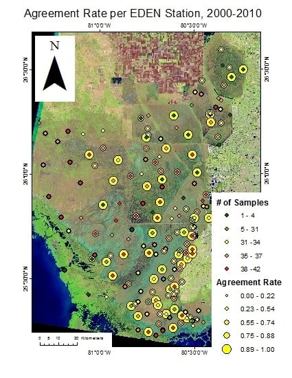


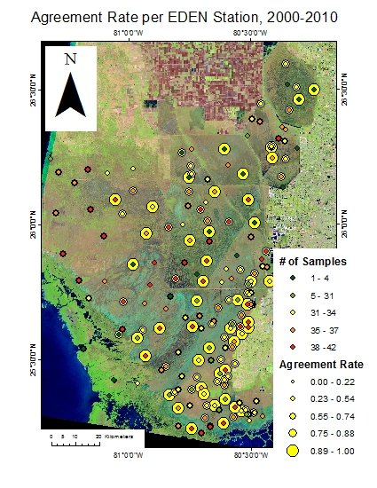
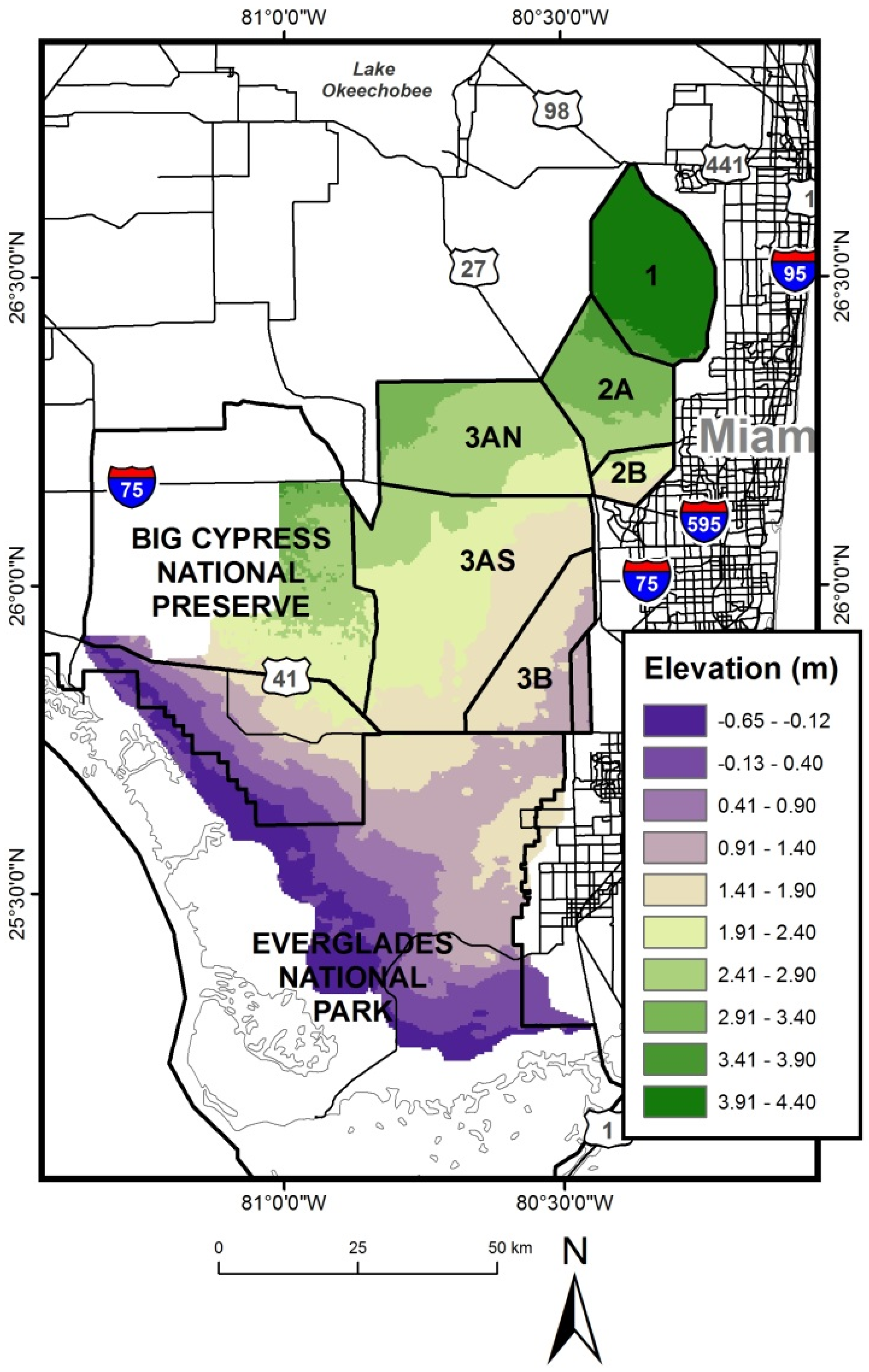
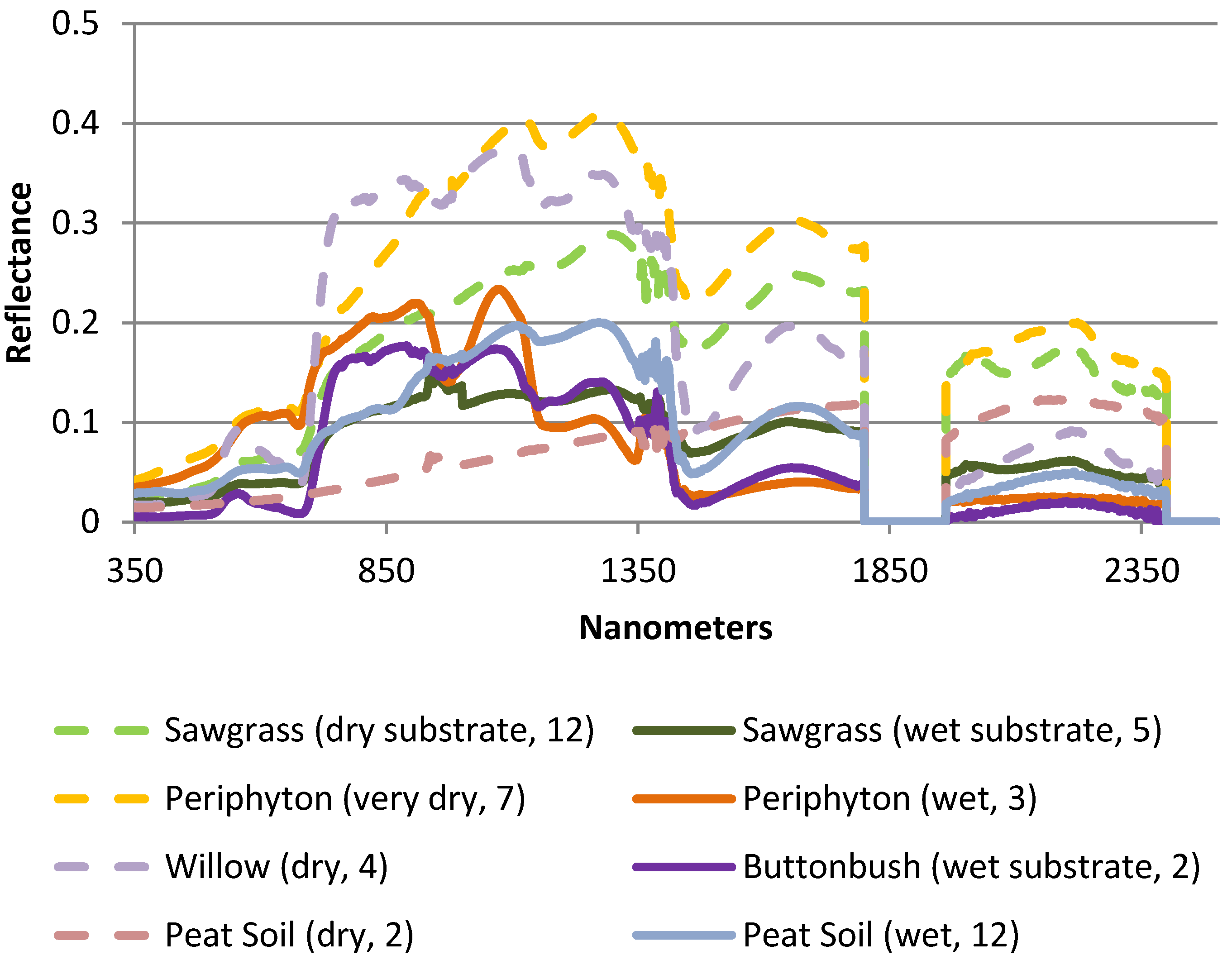
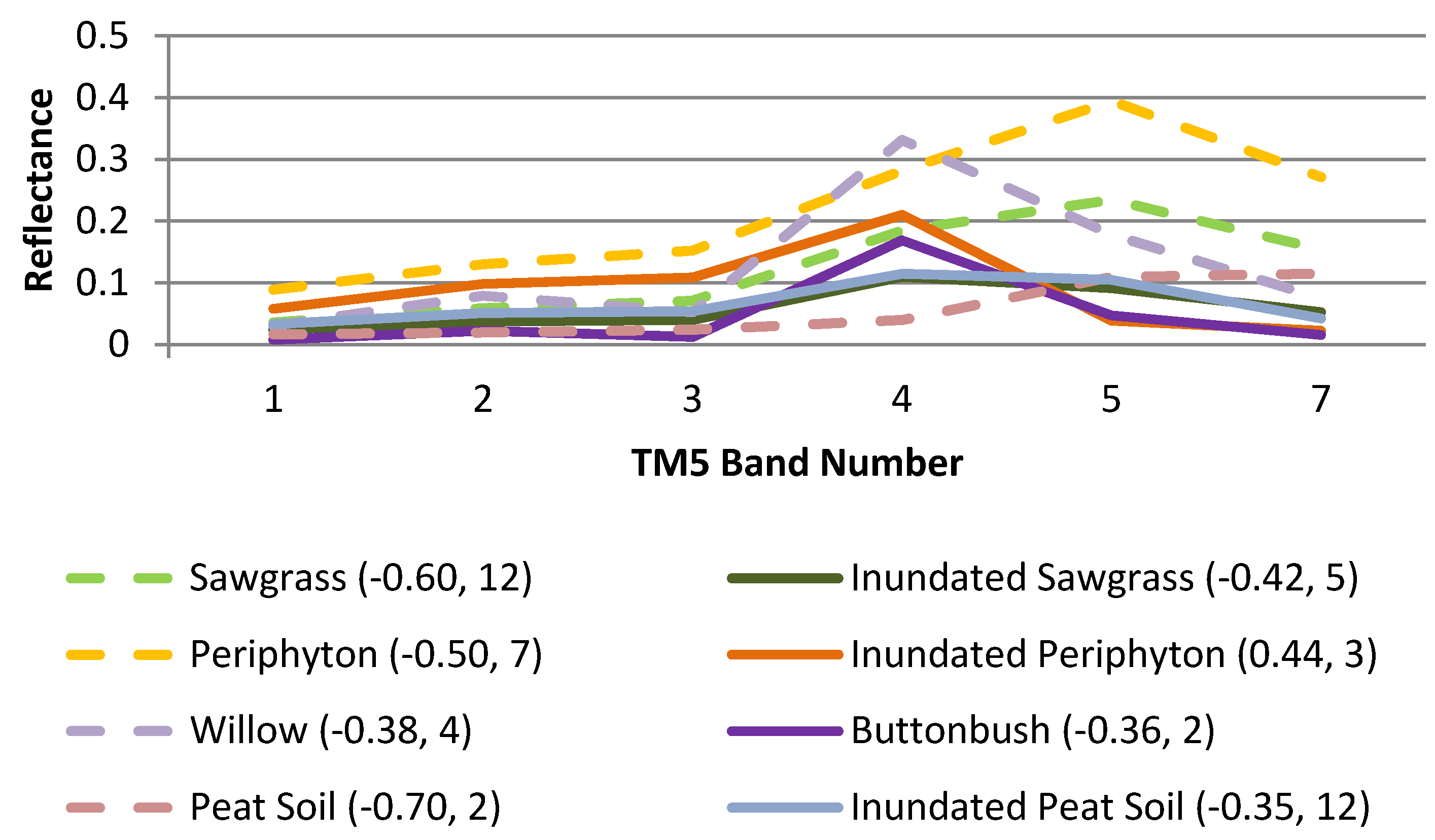
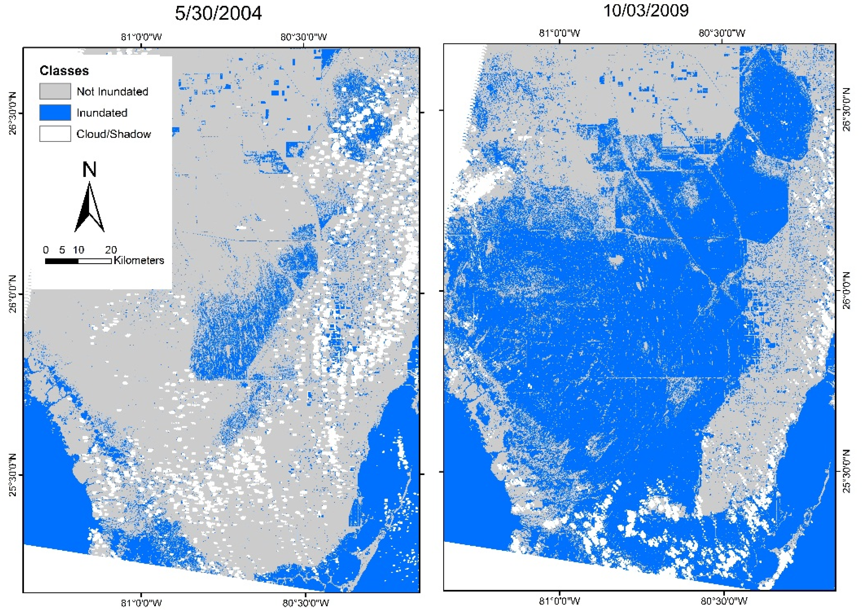
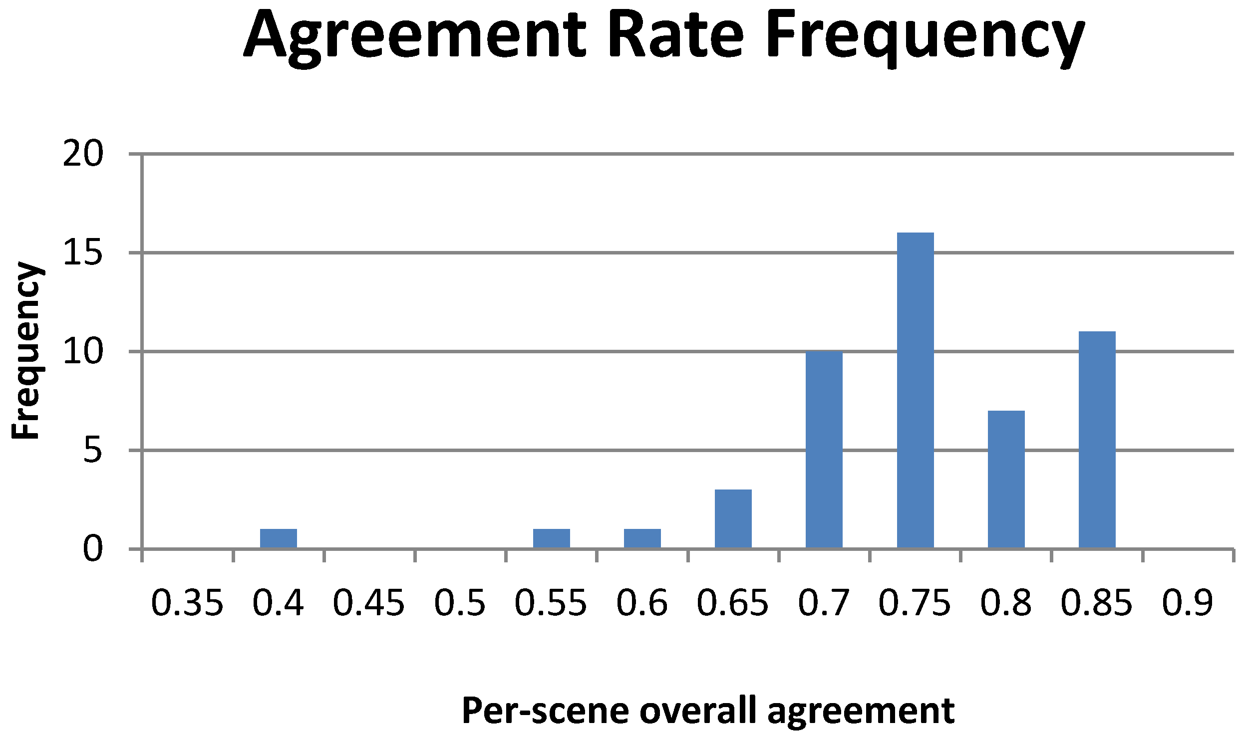
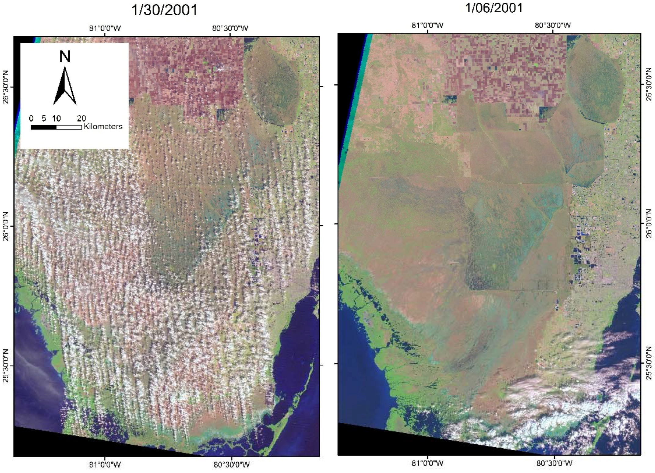
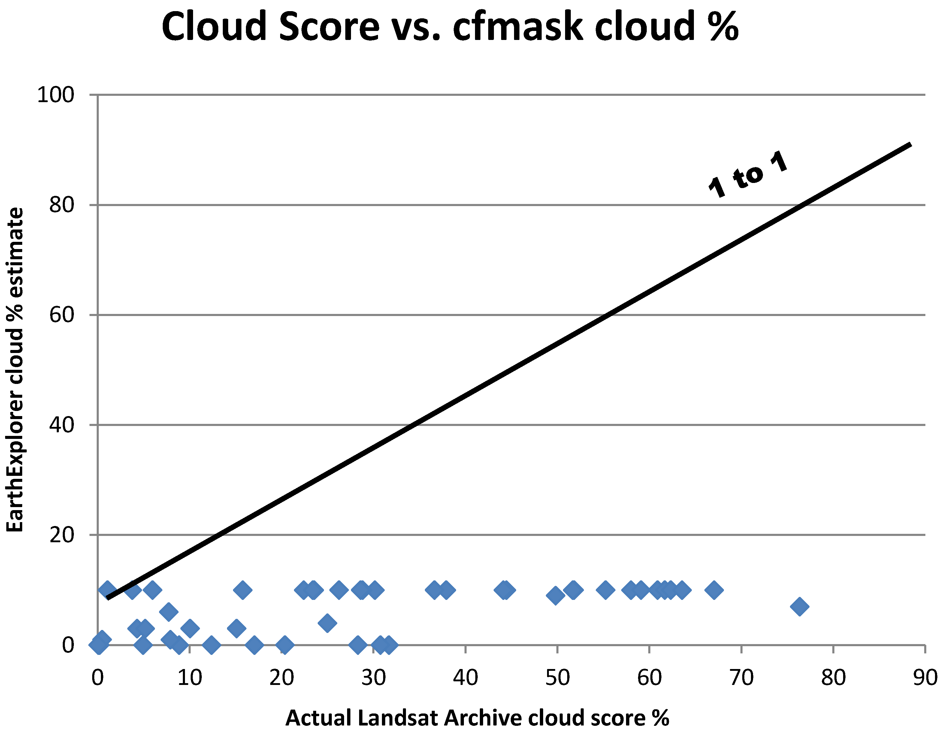
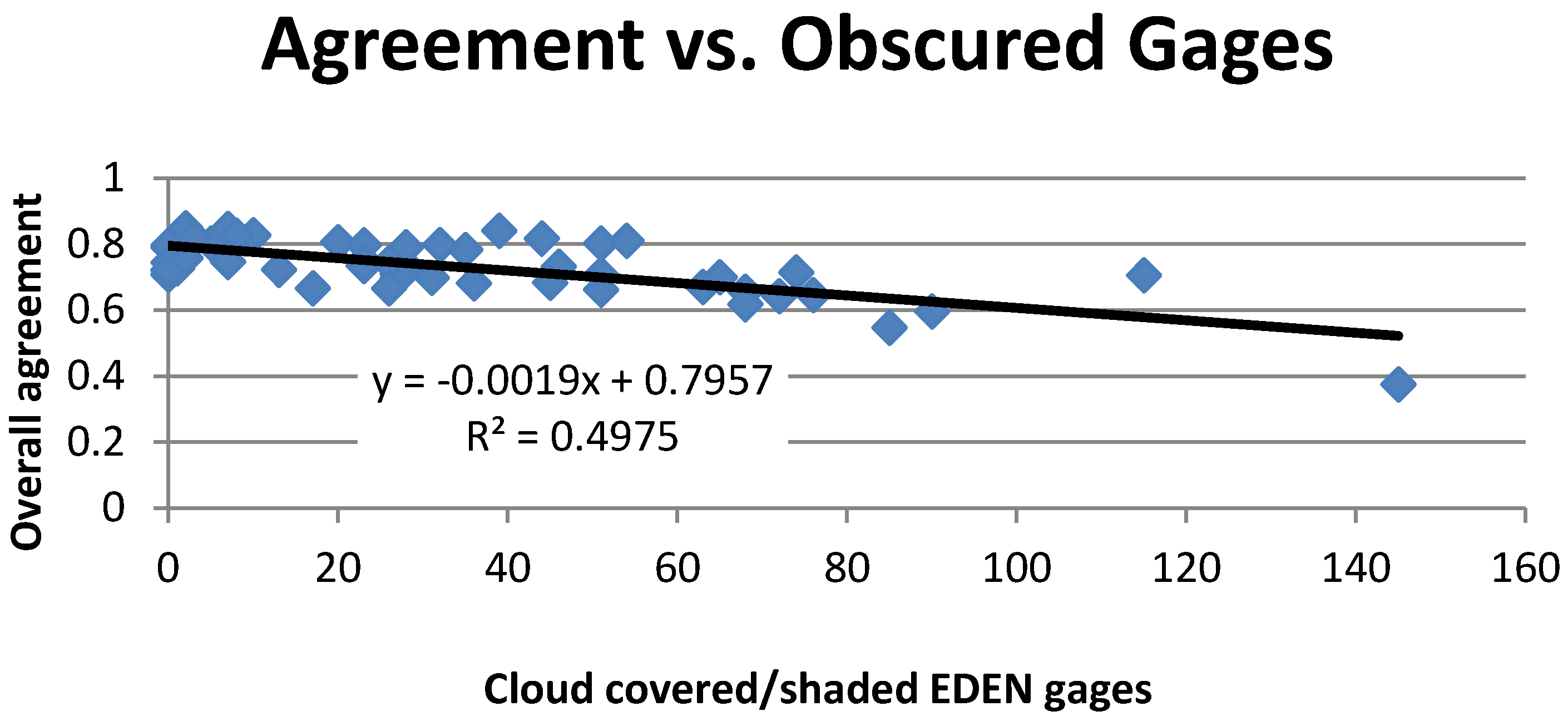
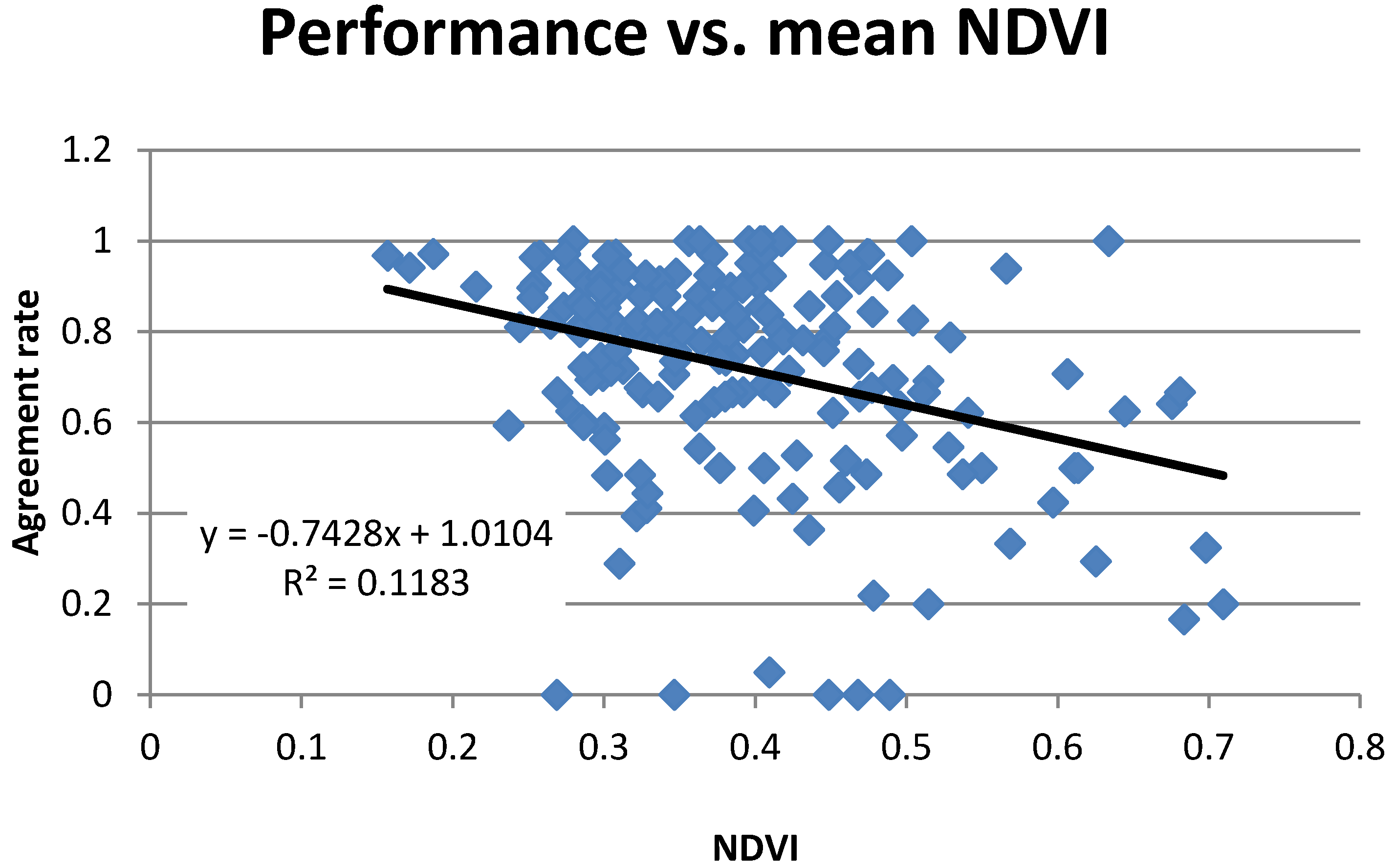
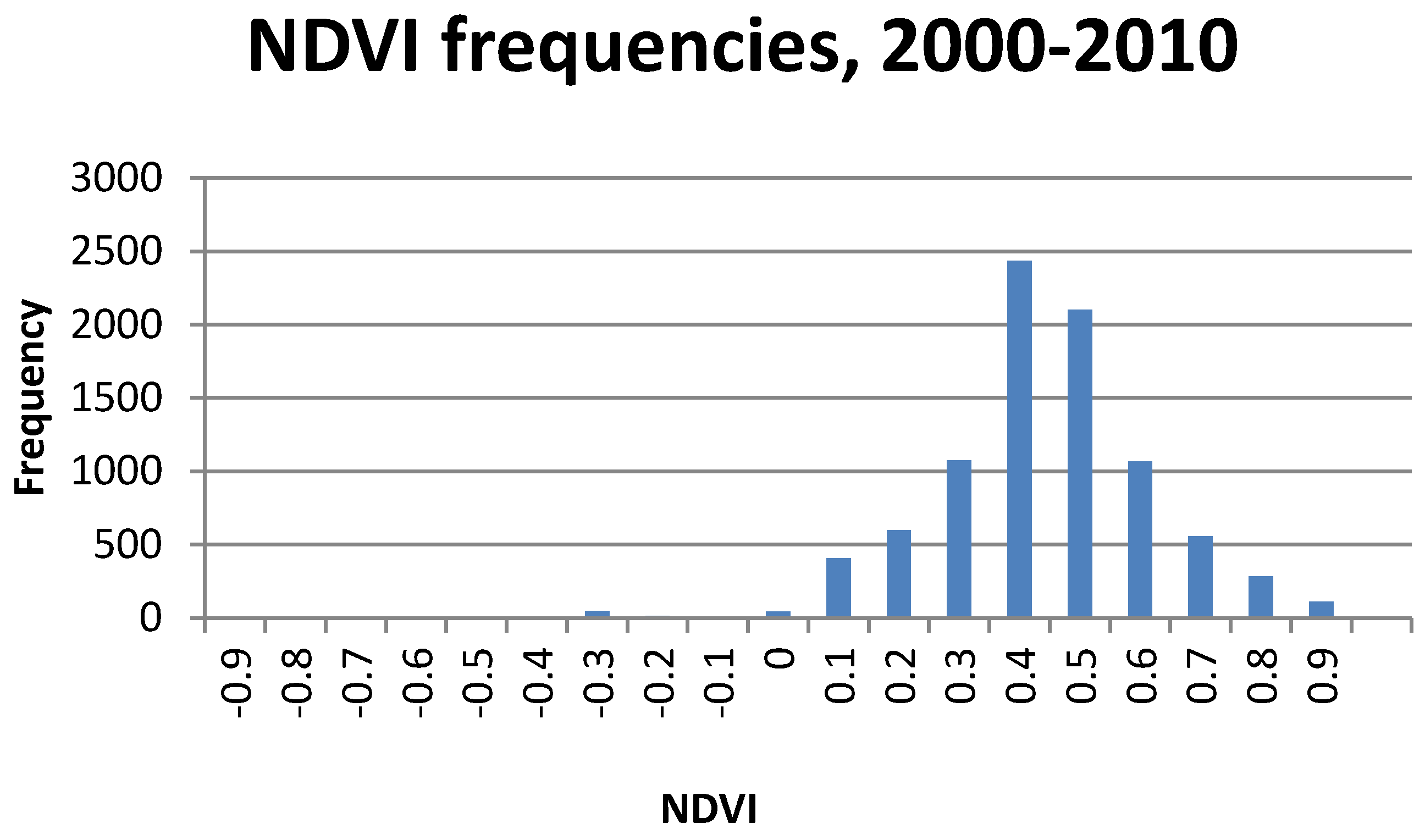
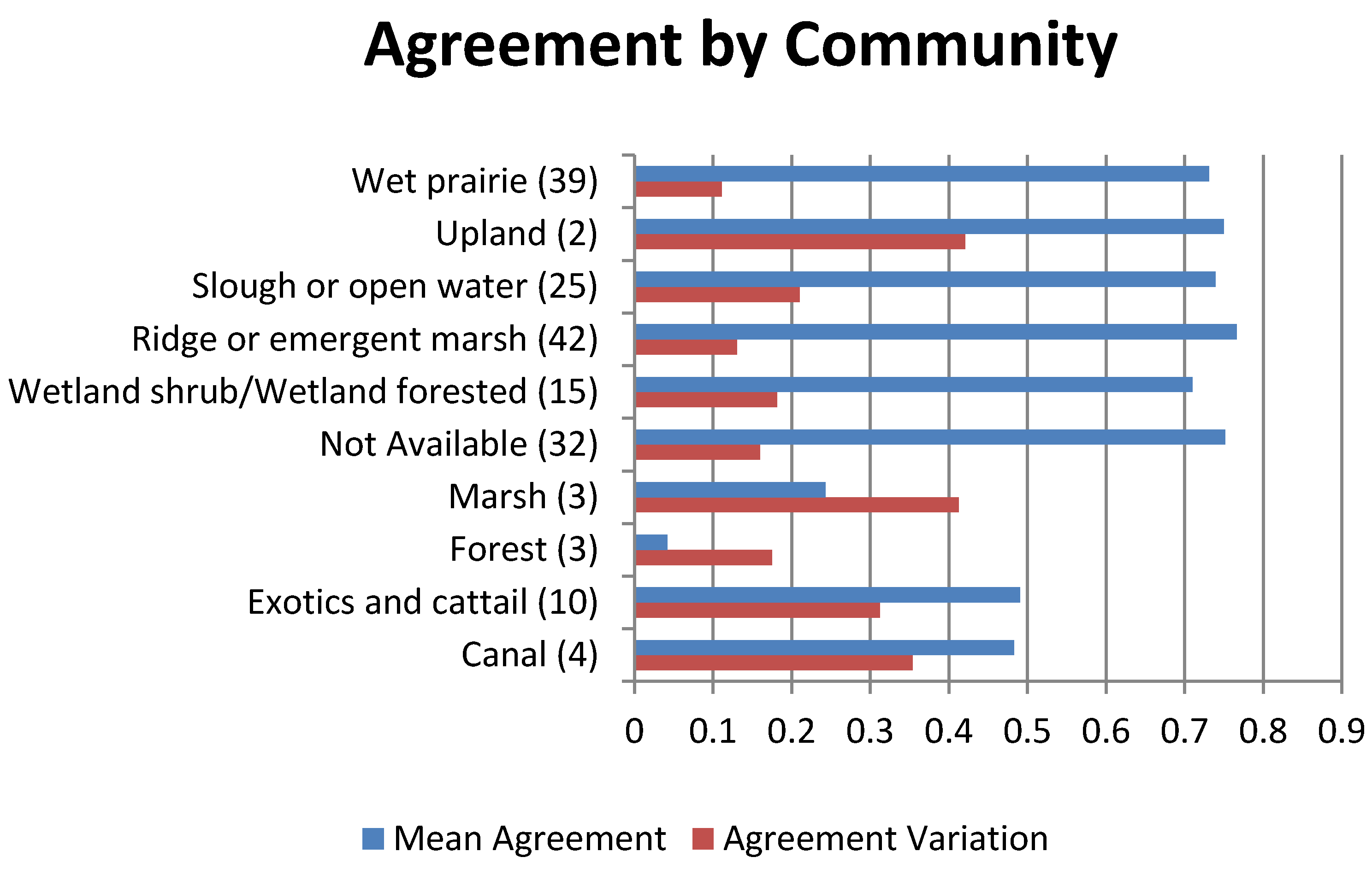
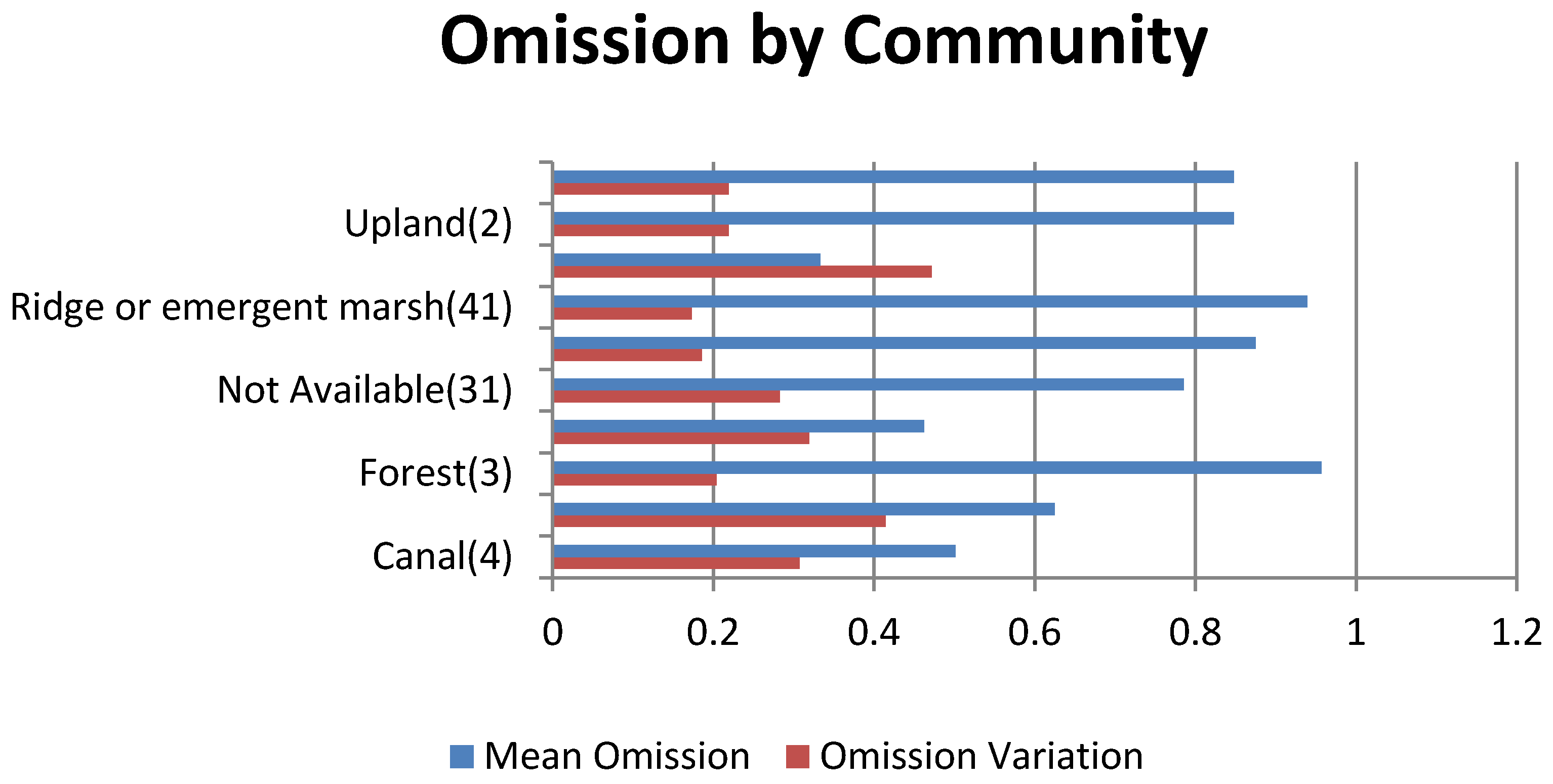
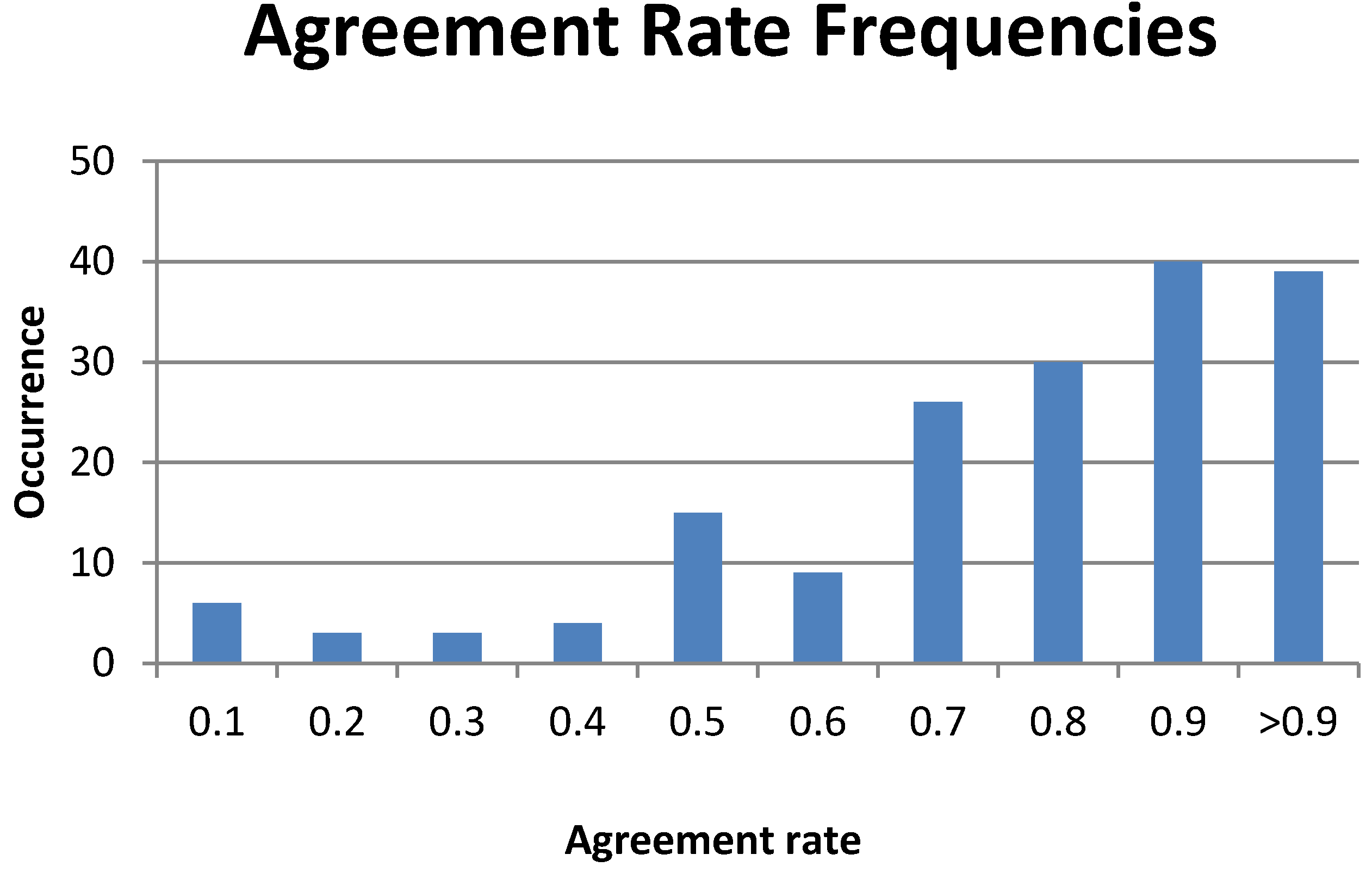
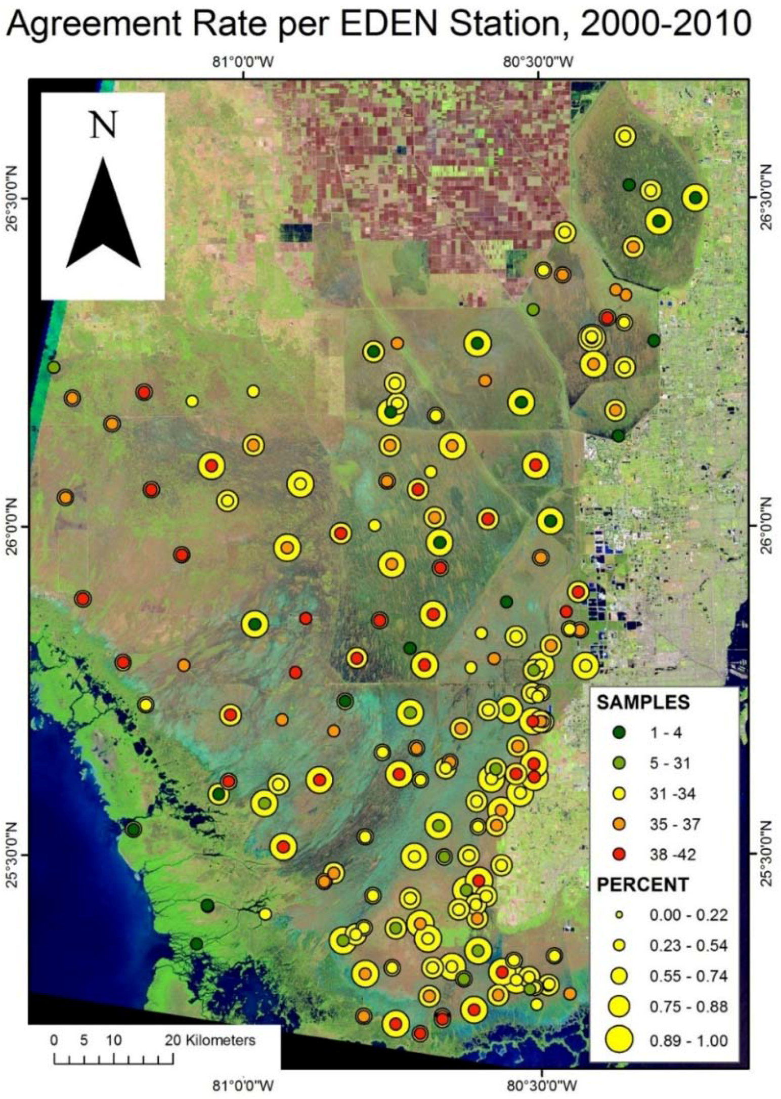
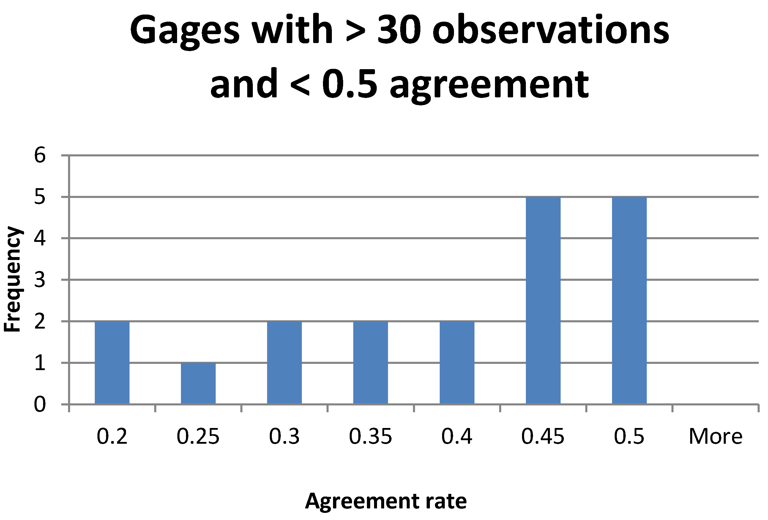
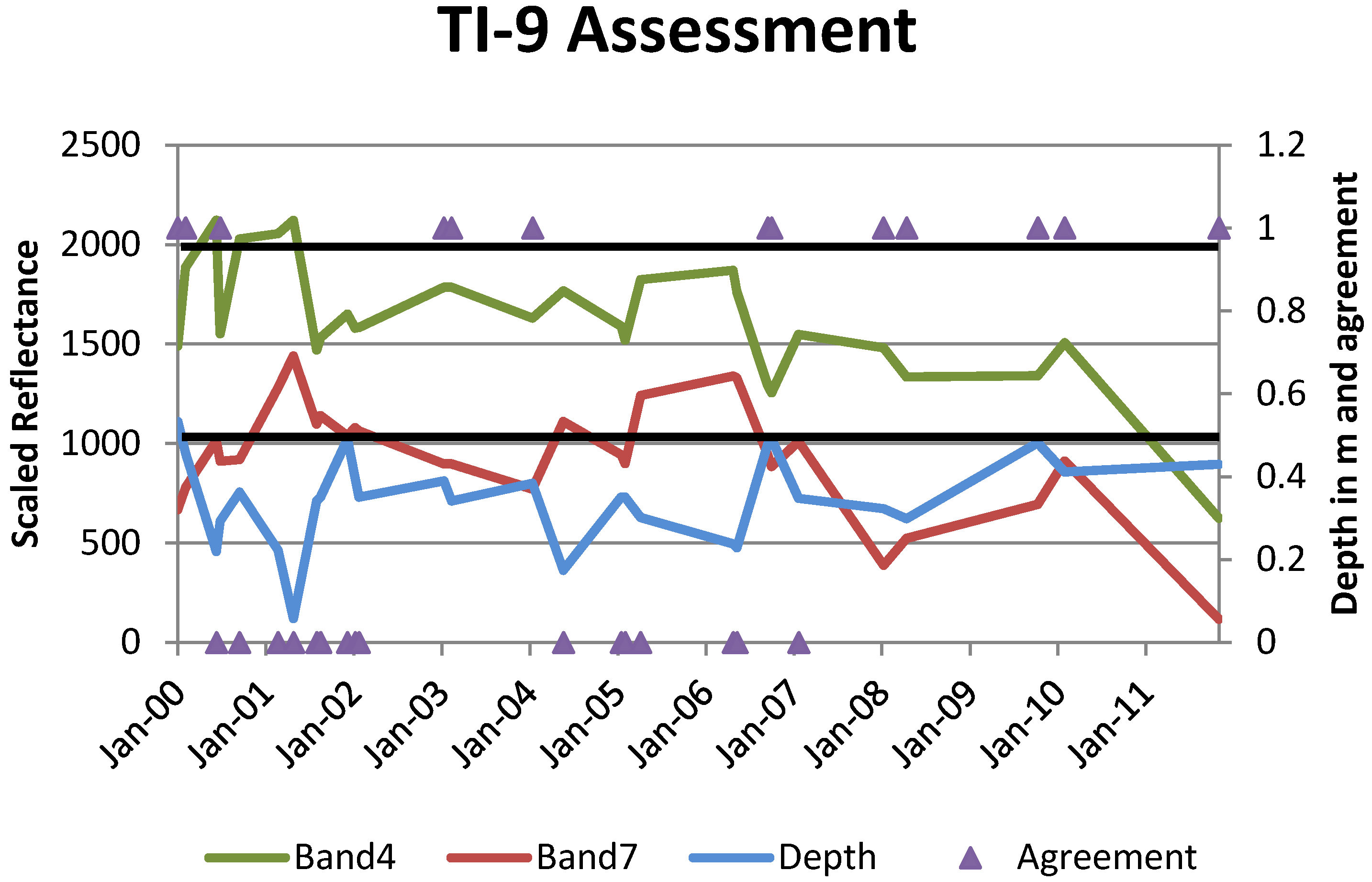
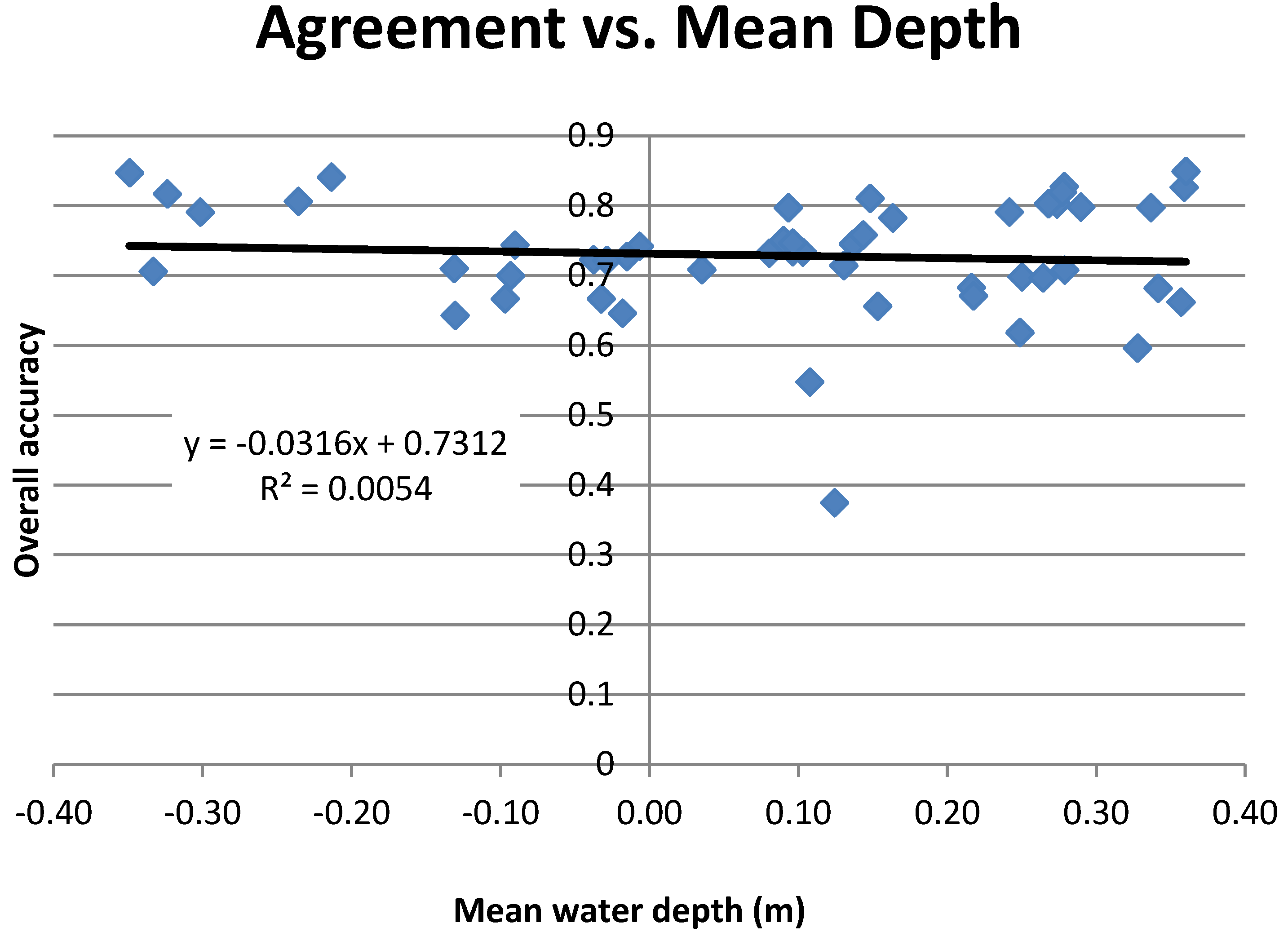
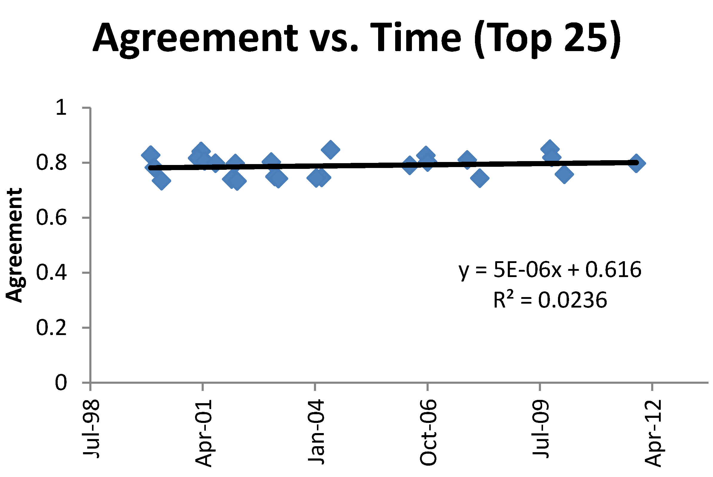


