Article

Long-Term Monitoring of the Flooding Regime and Hydroperiod of Doñana Marshes with Landsat Time Series (1974–2014)

by
Ricardo Díaz-Delgado
1,*,†,
David Aragonés
1,†,
Isabel Afán
1,† and
Javier Bustamante
1,2,†
1
Remote Sensing and GIS Laboratory (LAST-EBD), Estación Biologica de Doñana (CSIC), Avda. Américo Vespucio s/n, Isla de la Cartuja, 41092 Sevilla, Spain
2
Department of Wetland Ecology, Estación Biologica de Doñana (CSIC), Avda. Américo Vespucio s/n, Isla de la Cartuja, 41092 Sevilla, Spain
*
Author to whom correspondence should be addressed.
Remote Sens. 2016, 8(9), 775; https://doi.org/10.3390/rs8090775
Submission received: 31 May 2016 / Revised: 6 September 2016 / Accepted: 12 September 2016 / Published: 20 September 2016
(This article belongs to the Special Issue What can Remote Sensing Do for the Conservation of Wetlands?)

Abstract

:
This paper presents a semi-automatic procedure to discriminate seasonally flooded areas in the shallow temporary marshes of Doñana National Park (SW Spain) by using a radiommetrically normalized long time series of Landsat MSS, TM, and ETM+ images (1974–2014). Extensive field campaigns for ground truth data retrieval were carried out simultaneous to Landsat overpasses. Ground truth was used as training and testing areas to check the performance of the method. Simple thresholds on TM and ETM band 5 (1.55–1.75 μm) worked significantly better than other empirical modeling techniques and supervised classification methods to delineate flooded areas at Doñana marshes. A classification tree was applied to band 5 reflectance values to classify flooded versus non-flooded pixels for every scene. Inter-scene cross-validation identified the most accurate threshold on band 5 reflectance (ρ < 0.186) to classify flooded areas (Kappa = 0.65). A joint TM-MSS acquisition was used to find the MSS band 4 (0.8 a 1.1 μm) threshold. The TM flooded area was identical to the results from MSS 4 band threshold ρ < 0.10 despite spectral and spatial resolution differences. Band slicing was retrospectively applied to the complete time series of MSS and TM images. About 391 flood masks were used to reconstruct historical spatial and temporal patterns of Doñana marshes flooding, including hydroperiod. Hydroperiod historical trends were used as a baseline to understand Doñana’s flooding regime, test hydrodynamic models, and give an assessment of relevant management and restoration decisions. The historical trends in the hydroperiod of Doñana marshes show two opposite spatial patterns. While the north-western part of the marsh is increasing its hydroperiod, the southwestern part shows a steady decline. Anomalies in each flooding cycle allowed us to assess recent management decisions and monitor their hydrological effects.

Graphical Abstract

1. Introduction

Doñana temporary marshes are one of the largest protected wetlands in Europe with an extent of 340 km2, of which 300 km2 are included in the Doñana National Park. With a typical Mediterranean climate, the flooding cycle starts in September and usually reaches maximum flooding levels at the end of boreal winter, mainly driven by rainfall [1]. The dominant clay and silt substrates of Doñana marshes are soaked with the first showers and a shallow water layer (0.51 m average water column) spreads over the floodable area (Figure 1, solid blue area). In late spring, evaporation becomes the most important factor in the hydrological balance and the marshes dry up almost completely by the end of July. During summer, groundwater plays an important role in maintaining certain humidity levels at seepages [2].
Under natural conditions, interannual variability of continental wetlands is driven by meteorological conditions (rainfall or water table oscillations). However, Doñana marshes have experienced throughout the last century a continuous and severe transformation and degradation as result of human intervention (channelling of river arms, river course dredges, wetlands drainage for farming and aquaculture, widespread groundwater extraction, pollution spills, waterway shipping, etc.). Doñana marshes have undergone not only drastic reduction of the original extent (around 1500 km2 [3,4]) but also a permanent threat to the protected area, due to the progressive reduction of both water supply and quality. Overall, changes in the original marsh area at the beginning of the 20th century have led to the current 270 km2 occupied by shallow waters (with an estimated loss of 80% from its original extent). In addition to wetland area reduction, tidal influence, one of the main flooding drivers, was also controlled in 1984 by the construction of a dike along the right bank of the Guadalquivir River inside Doñana (Figure 1). Among such dramatic changes, a massive toxic spill in April 1998 to the Guadiamar River (the major tributary), led the scientific community and policy-makers to set up and implement an ambitious restoration program, named ‘Doñana 2005’, aiming at recovering the quantity and quality of the tributary waters entering these vast wetlands [1]. The project is still ongoing, assessing the success of restoration action.
Now more than ever we need to know the historical flooding patterns, both spatial and temporal, and their relationships with natural climatic variability or anthropic modifications (land use changes and water demand). Details on flooding process, such as interannual and seasonal variations, as well as the influence of human transformations have long been demanded by decision-makers in order to apply scientifically based management to the Doñana marshes. So far, hydrological management has been conducted on an “event–reaction” basis, leading to temporal solutions that afterwards became part of new problems [5]. Hydroperiod, the length of time each point remains flooded along an annual cycle [6], is a critical ecological parameter that shapes aquatic plants’ and animals’ distribution and determines available habitat for many of the living organisms in the marshes [7,8]. Annual hydroperiod is also the ultimate result of flooding dynamics due to human activities and global trends.
Thus, the sustainable management of the Doñana wetlands requires a better understanding of the structure and dynamics of the flooding process. This knowledge can be achieved through systematic long-term monitoring, although access limitations may make the cost of direct monitoring prohibitive. Remote sensing is cost-effective in terms of the extent surveyed and has the potential to scale up ground-based surveys and studies [9] by repeatedly imaging large areas. Many methods are available to represent accurately on-the-ground information and phenomena through collected imagery. One of the main advantages of remote sensing information sources comes from the possibility to access, for any place in the world, historical scenes revealing past land uses and cover.
Optical images have been widely proved to be an excellent tool to discriminate continental water bodies [10,11] from other targets, or to monitor inland water characteristics [12,13,14,15,16], but their use is less frequent for shallow wetlands covered by aquatic plants [17,18]. Many previous studies have used optical images to reveal and assess the damage caused by catastrophic floods as well [19,20]. Low reflectance in the Short Wave Infrared (SWIR) region (1.4–3 µm) is characteristically related to the presence of water [21]. However, several water characteristics such as depth and turbidity, as physical constraints, reduce the ability to discriminate accurately, in a simple way, shallow water’s extent [19]. In addition, shallow and clean waters make the bottom visible, which increases radiometric signal from the soil. Turbid waters usually show reflectance peaks between 700 and 900 nm, related to the presence of phytoplankton and/or suspended sediments [22,23]. Moreover, the presence of aquatic plants contributes to the noise when delineating wetlands due to their heterogeneous distribution. These constraints enhance the challenge of systematically producing flood maps for shallow wetlands such as the Doñana marshes.
Alternatively, many studies have relied on microwave imagery to map flood levels [24,25,26,27]. Radar sensors have several advantages over optical and thermal ones that make them particularly applicable to monitoring hydrologic conditions of wetlands. Radar imaging operates independent of cloud cover and solar illumination, and microwaves are very sensitive to the moisture content of the elements being imaged. However, wetlands usually present complex vegetation cover and structure patterns and differences in surface roughness that affect the way the microwave radiation interacts with the target and ultimately how much energy is returned to the satellite [28]. In addition, roughness caused by aquatic plants or wind on the water surface in shallow marshes may contribute to backscattering signal [29] according to the SAR band used. Despite such limitations, radar is being widely used for continental wetlands delineation in many studies [30,31].
Long time series of images have been stored and made available for several remote sensing sensors, allowing researchers to revisit any place in a former time. Moreover, for Landsat platforms, different sensors have been acquiring comparable images since 1972 [32]. This valuable spatial and temporal information is enhanced by spectral resolution, which makes Landsat remote sensing images a very useful tool for land cover change mapping [33]. In the case of large study areas, the cost-benefit rate rises when dealing with long-term monitoring programs and land use change analysis [34,35].
In this work we assess the performance of different digital image analysis techniques with Landsat images seeking to accurately determine flooded areas in the Doñana marshes. Different empirical modeling techniques and supervised classification methods were evaluated. Method selection was based on ground-truth assessment of different flood classes. Once the optimal method was selected, our main goal was to implement a semiautomatic procedure to produce systematically reliable and comparable flood maps of the Doñana marshes for the last 40 years [36]. The selected method should be consistent enough to be applied over a radiometrically normalized long time series of Landsat images. The resulting flooding masks allowed us to reconstruct historical flooding patterns and temporal trends for every single 30-m pixel in the Doñana marshes. Systematic flood mapping has enabled the reconstruction of an annual hydroperiod for every flooding cycle. This critical and ecologically meaningful variable is being used to assess the effects of global change processes and human management on the Doñana marshes.

2. Material and Methods
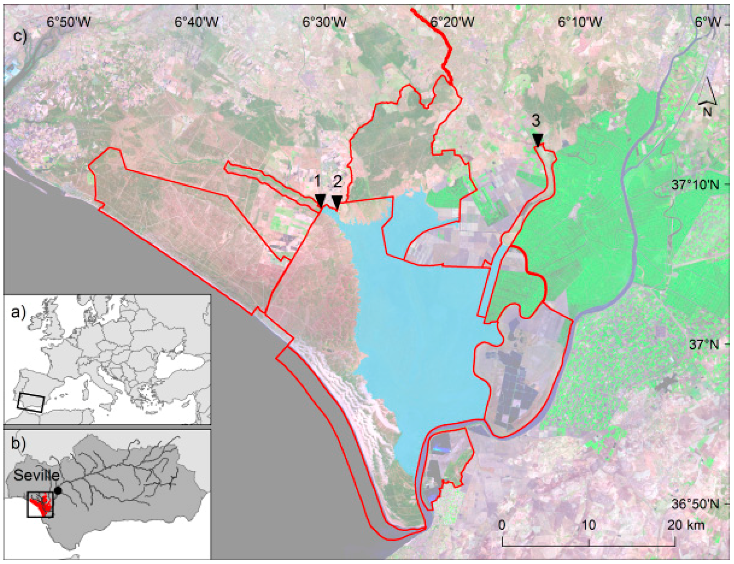
2.1. Study Area

The study area is located at the estuary of the Guadalquivir River (37°0′N 6°37′W), a large and shallow floodplain in Southwestern Spain (Figure 1). The Doñana marshes are a vast seasonal freshwater wetland of international importance, considered as Western Europe’s largest sanctuary for migratory birds. In 1969 they were declared a national park, then a Biosphere Reserve in 1980, an Important Wetland Site under the Ramsar Convention in 1982, and a Natural World Heritage Site in 1984 [1]. Doñana is also recognized as a Long-Term Socio-Ecological Research (LTSER) platform integrated in the LTER-Europe network [37] by applying harmonized protocols for long-term socio-ecological research.
The climate of the area is subhumid Mediterranean with Atlantic influence. The mean annual temperature is 17 °C, the coldest month is January with 10 °C, and the warmest month is July with 24 °C. The average annual rainfall is 550 mm, with dramatic interannual variation, going from 170 mm (2004–2005) to 1000 mm (1995–1996). Rainfall concentrates between October and April, whereas the dry season occurs from May to September [38]. The variable winter rainfall floods Doñana marshes, forming a wide floodplain that dries up during summer. Flooded areas are variable in depth, turbidity, and vegetation cover, being driven mainly by the amount and seasonal pattern of rainfall. In dry years, flooding occurs only on the sparsely distributed depressions (lucios) and historical tidal courses (caños). Maximum water volume may reach 265 hm3 during exceptionally wet flooding cycles such as the 1995–1996 one, achieving 2.47 m of water column at the deepest points, although average annual maximum depth is about 0.51 m for the whole marshes. Later in the season, the evaporation rate, going from 2 mm/day in January to 10 mm/day in July, controls the water bodies’ permanence [39].

2.2. Satellite Imagery

We acquired all available cloud-free Landsat MSS, TM and ETM+ scenes for Doñana National Park (Path: 202, Row: 34). Altogether, 462 images covering the 1974–2014 period form the time series for this study (70 MSS, 262 TM and 130 ETM+). From them, up to 71 scenes were discarded due to different and unexpected acquisition problems such as missing lines and columns, radiometric incoherences, line shifts, and cloud cover over the study area. The minimum number of scenes per year was three for 1980, while a maximum of 27 scenes was available for 2009; the average number was 10 valid scenes per year. The final number of valid scenes was 391, evenly distributed along the flooding cycle (December to May, 45% of total available scenes).

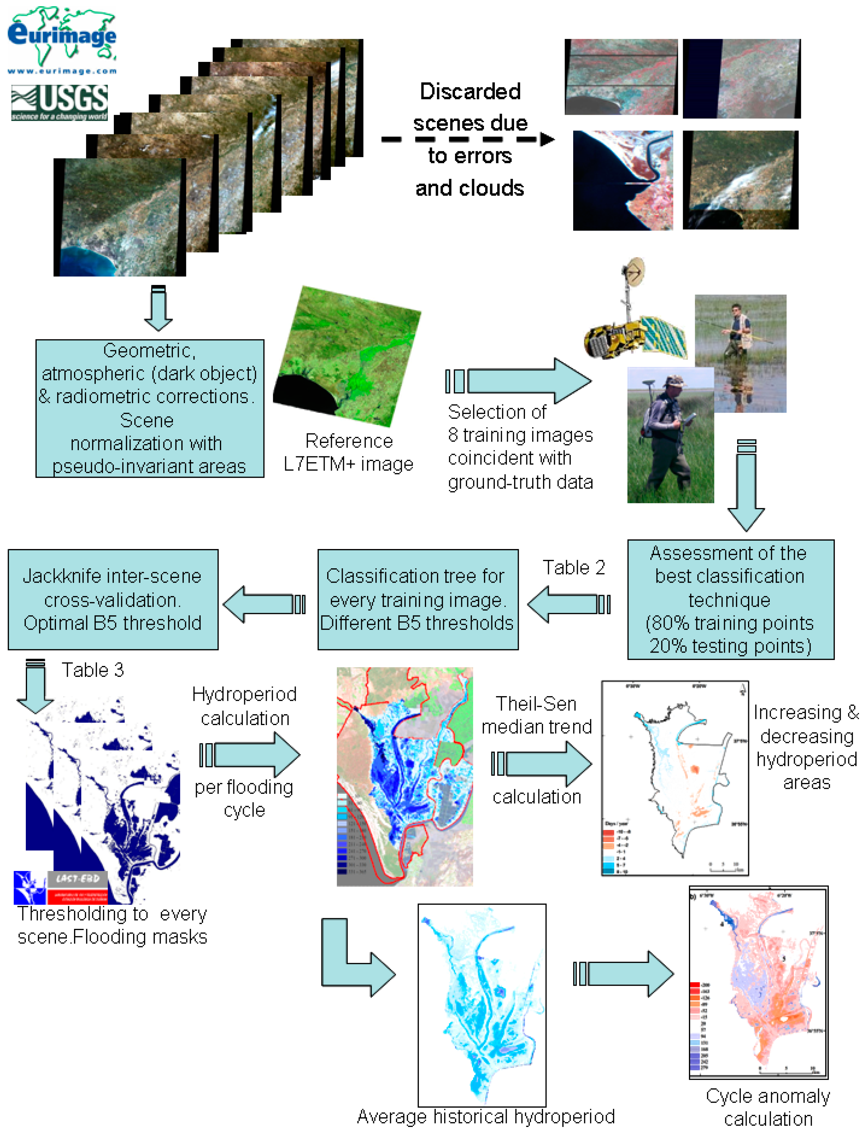
2.3. Image Processing

In order to make the time series comparable, a semi-automatic robust and coherent pre-processing protocol was applied. The complete procedure included metadata retrieval from raw 1G data images, geometric and atmospheric corrections, followed by time series radiometric normalization using ordinary least squares regression towards a reference cloud-free and clear atmosphere scene (18 July 2002 for Landsat ETM+ and TM images and 28 August 1985 for Landsat MSS images) using pseudo-invariant areas [40,41].
The panchromatic band (0.52–0.90 µm) of a Landsat 7 ETM+ image from 18 July 2002 was georeferenced with 100 ground control points (GCP) using the the 1998–1999 1:60,000 aerial orthophoto as reference [42]. The rest of the TM and ETM+ images were automatically co-registered to this reference image with RMSE < 1 pixel. The resampling method was cubic convolution in order to improve spatial coherence of final classification maps [43]. Average RMSE calculated with an independent set of GCP on co-registered images was 17.5 m. For MSS images we followed the same approach, using as reference a Landsat 4 summer scene acquired in 1985 by both sensors, MSS and TM, aboard the same platform. MSS output pixel size was set to 60 m × 60 m from the nominal 79 m × 57 m. RMSE for MSS co-registration was independently estimated in 23 m. For Landsat 7 ETM+ SLC-off images acquired after 31 May 2003 we applied gap filling based on the segmentation model approach [44]. Such a method does not use external data to interpolate gaps but segments from the original image elements. With a similar method Chen et al. [45] demonstrated similar land cover map classification accuracies compared to gap-free scenes.
Images were then atmospherically corrected and transformed into reflectance values using the Pons and Solé-Sugrañes [46] method based on the dark object model [47]. No topographic correction was applied since in the study area relief is negligible (the study area range being less than 10 m a.s.l.).
Finally, all the images were radiometrically normalized to allow comparisons across different sensors, dates, and atmospheric conditions by using a set of pseudo-invariant areas [40,48,49]. Pseudo-invariant areas comprised over 60,000 pixels inside the scene, covering the full reflectance range, and selected from eight area types: deep sea, reservoirs, sand dunes, rocky outcrops, bare soils, airport runways, urban areas, and open mines [22]. They were confirmed to have low seasonal changes in reflectance and to be present from the beginning of the image time series. The method includes a cloud masking process based on empirical slicing of the Landsat thermal and red bands. Accordingly, pseudo-invariant pixels were rejected whenever covered by clouds. We used the same Landsat 7 ETM+ image as the radiometric reference image, which provided a high sun angle and overall good radiometric quality. For every combination of scene and band, we calculated a linear regression model using all pseudo-invariant pixels. Pixels with regression residuals greater than 1 Standard Deviation were assumed to have changed significantly in reflectance between the scenes and were therefore rejected. Once removed, a new regression model was then adjusted. Offsets and gains from the fitted regression models were used to normalize the time series of images to the reference one (band to band processing). More than 97% of the scenes bands were fitted with R2 values greater than 0.90. As expected, offset values were consistently lower for winter scenes. Certain bands of up to 18 scenes could not be normalized due to radiometric inconsistencies and they were discarded.

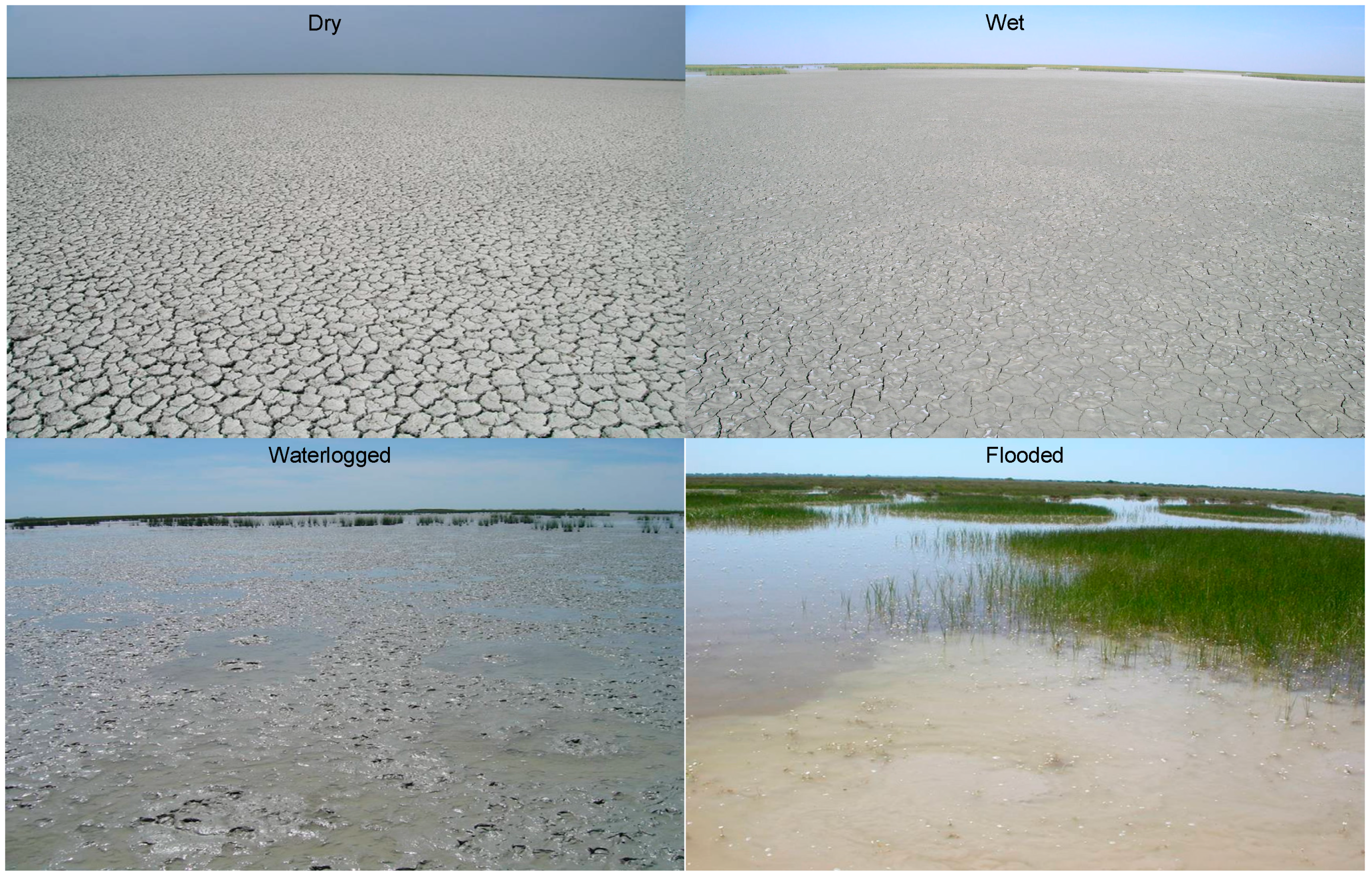
2.4. Ground Truthing

The Doñana marshes are a highly dynamic seasonal wetland. They may appear as a dry cracked clay soil in summer, bare water pools during the flooding season, or pools densely covered by emergent and floating plants. In addition, the marshes usually exhibit patchy turbidity patterns due to differences in suspended sediment concentrations (Figure 2). In order to capture such variability, we carried out 31 extensive ground-truth field campaigns coincident with 29 different Landsat overpasses (17 TM and 12 ETM+) from 2003 to 2013.
Ground-truth transects were designed to cross heterogeneous flooded areas and sampled simultaneous or recently after a satellite overpass. Sampling points were taken every 60 m in homogeneous covers collecting field information from a radius of 15 m, representative of the 30 m × 30 m Landsat TM and ETM+ pixel size. In order to collect the complete flooding gradient we recorded four different flooding classes (Figure 2) in relation to the percent of soil covered by water: dry soil (0%), wet (1%–25%), waterlogged (25%–75%), and flooded (>75%). Additionally, we recorded ancillary information on many other relevant variables such as water turbidity, water depth, percent of bare ground, plant and open water cover, and plant species abundance and dominance (Table 1). Such complementary information might help in assessing the discriminative ability of flooded pixels under different conditions. Geolocation of every point was recorded by means of PDA-GPS units with less than 4 m horizontal position error on average.
A total of 6005 field sampling points were collected by transects on foot and on horseback—and, in certain flood occasions, by canoe—to extend the ground-truth dataset. Ground-truth data were used to train (80% of the sample) and validate (20%) the classification procedures.

2.5. Flood Mapping and Accuracy Assessment

Clear water bodies have a very low reflectance in the optical spectrum, especially in the Near and Mid Infrared bands (bands 4, 5, and 7 of TM and ETM+). Reflectance in the visible and IR regions depends on the reflectance of the submerged soil, the water depth, the amount of suspended particles, and their optical properties [50,51]. The abundance of optically active components, such as phytoplankton, suspended minerals, and dissolved organic carbon directly affect water turbidity and colour [52]. The more turbid water bodies have higher reflectance values in the green and red visible bands [22].
Several procedures have been proposed to identify shallow inundated areas based on the low reflectance values of water bodies in the SWIR (Short Wave InfraRed) region. We tested various optical indices proposed in the literature ([53,54,55]) and several empirical classification approaches (Maximum Likelihood, Discriminant Function Analysis, and Logistic Regression using all six Landsat optical bands, and Classification Trees [18] using Landsat TM and ETM+ band 5) to automatically determine the flooding level in Landsat scenes. Kyu-Shun et al. [56], working in shallow wetlands with different turbidity levels, showed that Landsat TM band 5 (1.55–1.75 µm) is less sensitive to sediment-charged waters and therefore the best at delineating the limits between water and dry ground in turbid waters. Similar results were found by Bustamante et al. [57], showing that a classification tree on band 5 of Landsat TM and ETM+ sensors performed better when discriminating the Doñana shallow flooding levels.
As our study is focused on flood and hydroperiod mapping, we generated from the four flooding classes a simple flooding binary masks by merging the dry and wet classes as non-flooded and the waterlogged and flooded classes as flooded class.
We tested the different classifiers on a set of eight Landsat TM and ETM+ scenes (between 2004 and 2007) with coincident ground-truth data identifying flooded and non-flooded classes. The set of scenes was selected in order to use a balanced sample of ground-truth points (flooded vs. non-flooded), to work with exact matching between acquisition dates and sampling dates (see Table S1 for acquisition dates and ground-truth data). We built up classification trees with every band 5 of the training images by using a subset of ground-truth data as training sample (80% of points). For every scene we obtained different thresholds to provide the two classes: flooded and non-flooded. Classification trees on band 5 for every training date provided slightly different threshold values. Classification performance was assessed with coincident ground-truth observations for every single scene. Predictive accuracy was assessed using a random set from 20% of all sampling points (183 samples) and by computing the Cohen’s Kappa statistic [58] in order to measure the degree of agreement between classified and observed data and to test whether the prediction exceeded one that could be produced by chance alone (where k = 1 means perfect agreement and k = 0 no more agreement than by chance alone). Additionally, confusion matrices were calculated to retrieve Global Accuracy Values for every single classification tree, as an additional measure of the total accuracy of the classified maps [59].
However, in order to select the best threshold for the whole time series, we carried out a global accuracy assessment by following a Jackknife inter-scene cross-validation approach [18,60,61] (Figure 3). The proposed threshold should be consistent throughout years, sensors, illumination angles, and land cover changes. The Jackknife procedure estimates the classification agreement for each subsample of images omitting the ith observation to estimate the previously unknown agreement value. This inter-scene cross-validation consisted of three steps:
  • Computing classification trees, using the whole set of training images except for one of them each time, which was used as a validation image.
  • Computing the classification tree using all the training images.
  • Evaluating threshold accuracies from the all training images classification tree over the validation image with the ground-truth data for the corresponding date.
Once the optimal threshold was selected we applied it to the whole time series of images. Finally, as our study area corresponds to the Doñana marshes, we built up a background mask with the limits of the marshes, excluding the surrounding area where a network of water ponds may appear as flooded. Such a binary mask was systematically applied over every resulting flooding mask.

2.6. Hydroperiod Mapping and Trend Analysis

Once the best flood mapping method was identified, we applied a simple method to retrieve hydroperiod value (H) per pixel for every flooding cycle (Hc). We computed Hc according to the following equation:
H c = i = 1 n 1 ( D o C i + 1 D o C i ) = ( D o C 2 D o C 1 ) + + ( D o C n D o C n 1 )
where DoC stands for Day of Cycle (flooding cycle is set to 1 on the 1st of September of the previous year and to 365 on 31st of August of the year that follows). For every flooding cycle, the ith image corresponds to the first date the pixel was classified as flooded, while the n image is the last date when the pixel was labelled as flooded. The n value may eventually equal the total available number of flooding masks per cycle when a pixel is classified as flooded at every flooding mask for the complete flooding cycle. The procedure assumes constant flooding for a pixel classified as flooded between two consecutive available scenes. We calculated two different indexes in order to assess the representativeness of Hc for inter-cycle comparisons:
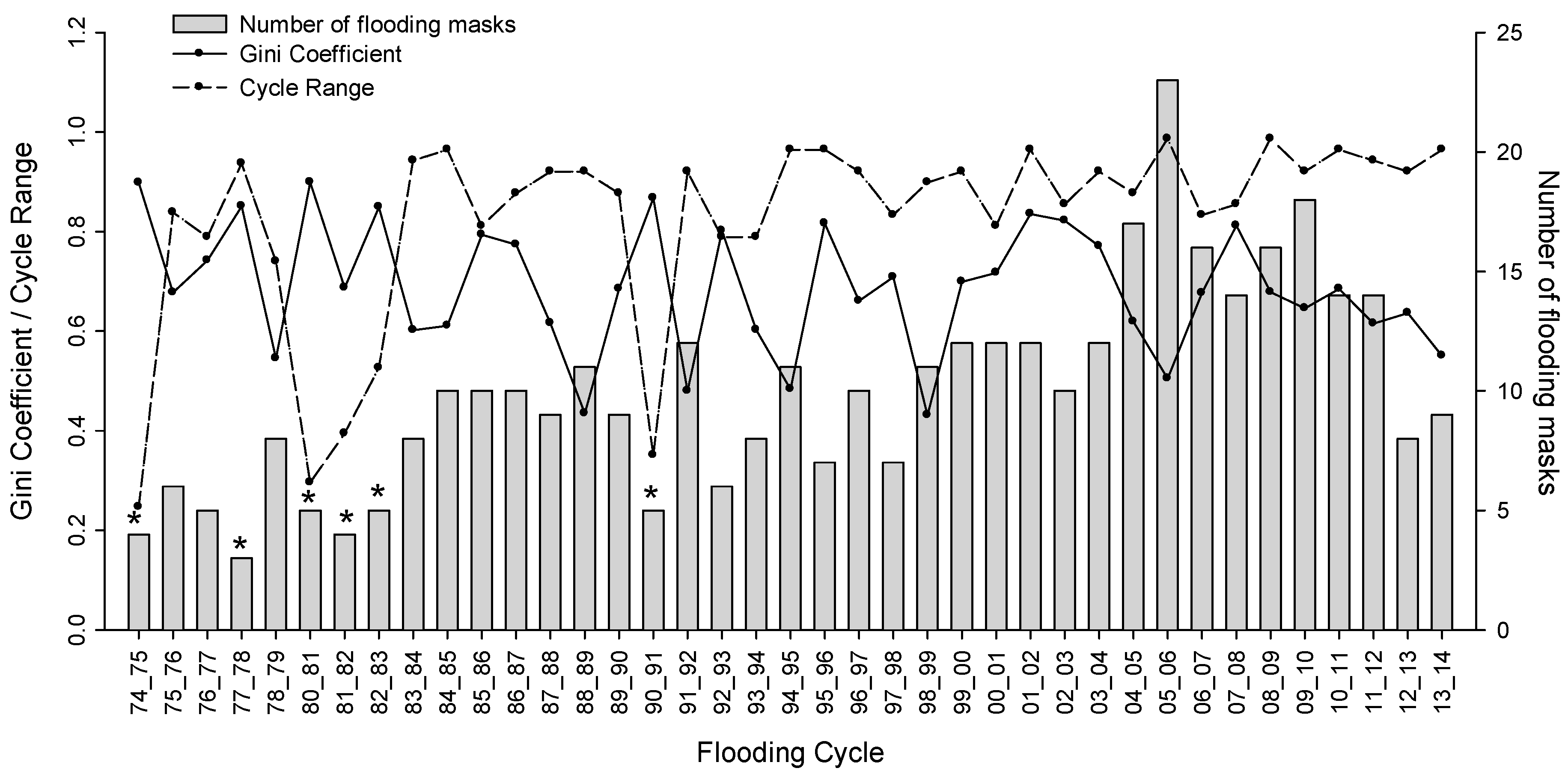
  • Cycle range (Cr): the ratio between the DoC range (earliest available date minus latest available date) per cycle and the complete cycle value (365 days). This index provides a rapid assessment of the percentage of the complete cycle covered by the first and last flooding mask available for each cycle.
  • Gini Index [62]: Calculated as the area under the equality curve and the cumulative proportion of available dates in relation to possible dates (22 Landsat MSS or TM acquisitions for a complete flooding cycle from 1974 to 1998 and 45 Landsat TM and ETM+ acquisitions from 1999 to 2011). The Gini Index provides a quick assessment on the evenness of available flood masks along the flooding cycle (values from 0 to 1). The higher the Gini Index for a cycle the lower the representativeness of the Hc values.
A low number of flood masks per flooding cycle produced a systematic bias in permanent inundated areas like the ocean or the river. In order to remove such bias we applied a linear stretch to the Hc estimate multiplying Hci by 365 and dividing by Hcmax, with Hci the value of the pixel and Hcmax the maximum value of Hc obtained for permanent waters like the sea. Such post-processing eliminates this systematic bias for the initial flooding cycles in the time series with a low number of flood masks.
Final hydroperiod maps indicate the number of days a pixel was detected as flooded (from 0 to 365) during the flooding cycle. Independent accuracy assessment of hydroperiod estimates by remote sensing was carried out using historical readings of water column values from a network of permanent limnimetric scales distributed across the Doñana marshes (see Figure S1 containing a location map of the scales in the marsh together with an example of a full flooding cycle reading values). Fixed limnimetric scales are periodically visited and the water column recorded by national park rangers. We selected the readings of the N28 limnimetric scale (Figure 4) since it has been agreed to be the most representative of the flooding levels for the whole marshland. In addition, N28 is the one with the longest continuous record of readings (1394 readings from 1995 to 2009). From such data, the ground-truth hydroperiod was therefore calculated by subtracting the last flooding day (water column reading = 0 cm) from the first observed flooding day (water column reading > 0 cm).
Time series of annual hydroperiod maps were used to calculate the Theil–Sen median trend, which uses a robust non-parametric trend operator highly recommended for assessing the rate of change in short or noisy time series [63]. Theil–Sen analysis calculates the slope of the trend from the median value of every pairwise combination of cycles. An interesting feature of the median trend is its breakdown bound. The breakdown bound for a robust statistic is the number of wild values that can occur within a series before it will be affected. For the median trend, the breakdown bound is approximately 29%. Thus the trends expressed in the image have to have persisted for more than 29% of the length of the series in flooding cycles (i.e., more than nine years for Doñana marshes).
Finally, in order to assess significant interannual changes, we computed hydroperiod anomalies for every flooding cycle as the difference between Hc and the mean hydroperiod of the whole time series [64]. For comparison purposes, MSS flooding masks were resampled to 30 m pixel size.

3. Results

3.1. Flood Mapping and Global Accuracy Assessment

Table 2 shows the mean global accuracies and mean Kappa values for every classification method. We chose a classification tree as the most accurate according to high Kappa and global accuracy and low variance.
The Jackknife inter-scene cross-validation procedure allowed us to derive the most accurate classification tree threshold value for the normalized band 5 of Landsat TM and ETM+ sensors (ρ < 0.186) for all the scenes with an average Kappa value of 0.66 and an average global accuracy of 94% (Table 3). The same process was applied to band 4 of Landsat MSS (0.8–1.1 µm) images, which provided a MSS band 4 threshold value of 0.10. Overall, the threshold reflectance values computed for single training scenes were lower than those calculated for training scenes. Such results indicate a much higher consistency expected for the threshold applied over the complete time series of images.
Final binary flood masks were calculated by applying the selected threshold to band 5 of the 345 Landsat TM and ETM+ images from 1984 to 2014 and the ρ < 0.10 threshold to band 4 of the 46 Landsat MSS images from 1974 to 1984.

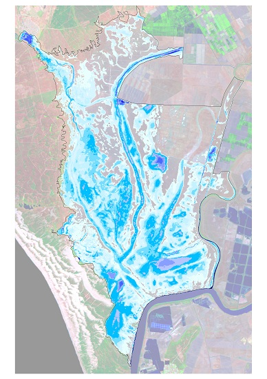
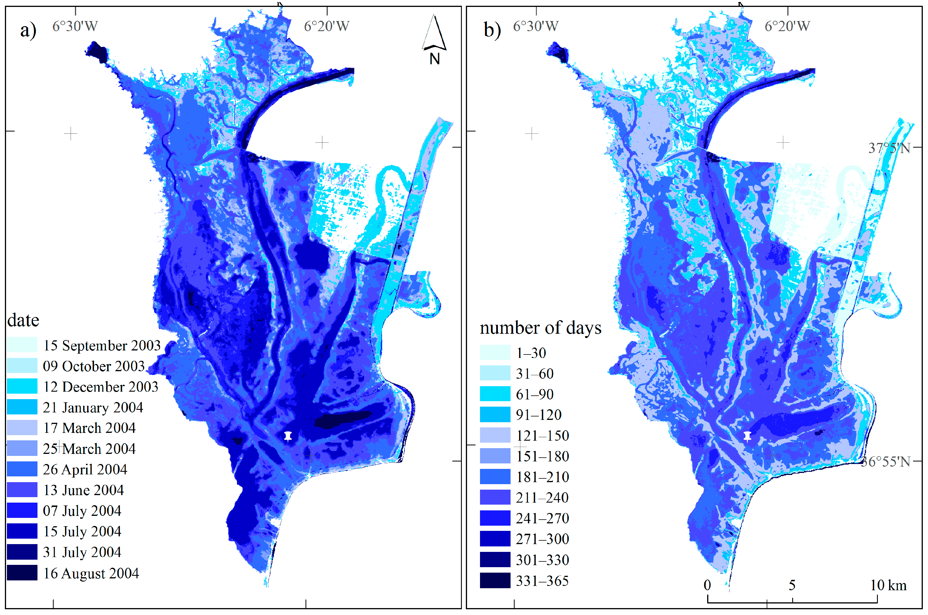
3.2. Hydroperiod Mapping

Figure 4a shows, as an example, the overlay of the 2003–2004 flooding masks; Figure 4b depicts the corresponding hydroperiod map. The hydroperiod map (Figure 4b) provides a more reliable and synoptic picture of the spatial distribution and duration of Doñana marshes flooding than the simple overlay of flooding masks. While the hydroperiod map provides quick information on how long every pixel was flooded for the selected cycle, the overlay of flooding masks does not allow us to visualize the whole extent of a single date because of overlying constraints.
Hydroperiod estimated from flooding masks derived from satellite images showed a significant and positive correlation with the one calculated from limnimetric readings (r2 = 0.90, p < 0.005, n = 13).
Hydroperiods between 1974 and 2014 were calculated for every flooding cycle except for the 1974–1975, 1977–1978, 1980–1981, 1981–1982, 1982–1983, and 1990–1991 cycles. We discarded these cycles because of the low total number of available flooding masks and the small Cycle Range and Gini coefficient values (Figure 5).
Once computed, mean hydroperiod and maximum flooded area per cycle showed a significant positive relationship with total rainfall during the flooding cycle (R2 = 0.36 and R2 = 0.56, respectively; p < 0.005, n = 33; see Figure 6). Yet there is still ca. 64% of unexplained hydroperiod variability that might be linked to non-coherent marsh trends and consequently to management actions or, less likely, to accumulated error in flood mapping and hydroperiod calculation. Although long assumed to be steadily increasing [65], the global mean marsh hydroperiod (with non-flooded pixels in the marshes accounting for 0) did not show any significant temporal trend. However, such global indicators may be hiding local opposing trends, which makes it essential to assess spatial variability along the time series.

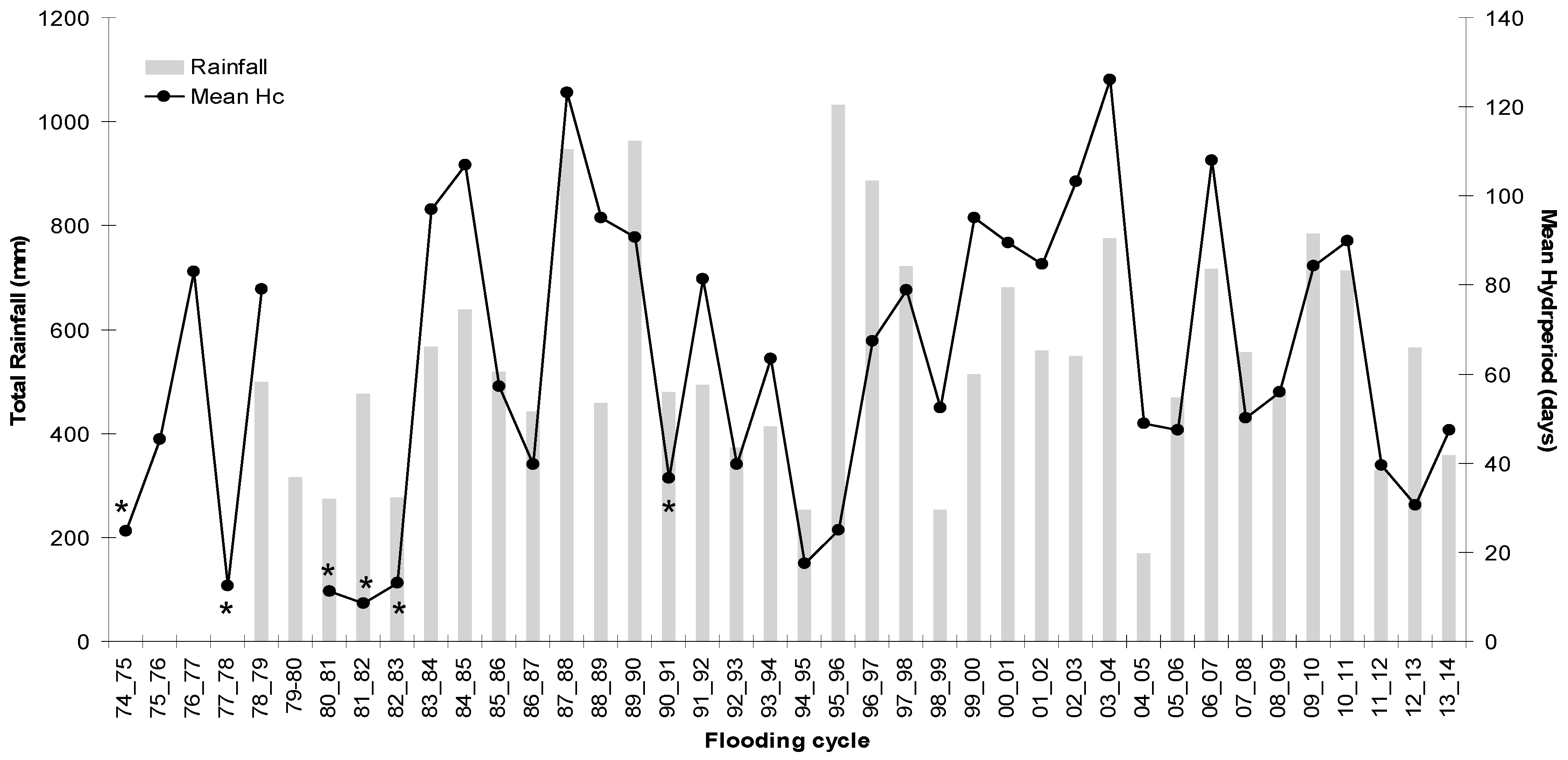
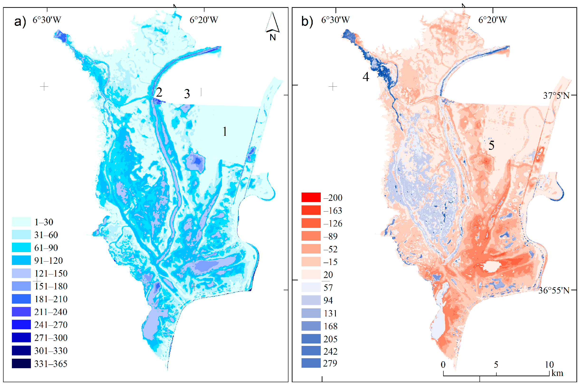
3.3. Hydroperiod Historical Trend and Anomalies

We evaluated interannual variation on hydroperiod dynamics by estimating the time series mean hydroperiod from 1974 to 2014 (excluding the previously mentioned cycles) and calculating the hydroperiod anomalies per flooding cycle (Figure 7).
Mean hydroperiod still reveals the dominance of hydrological features such as caños and lucios with higher hydroperiod values. The relationship with the marsh Digital Elevation Model derived from LiDAR [66] showed a tight correlation between microtopography and hydroperiod (r2 = 0.90, p < 0.001). The remaining unexplained variability might well reflect the wind drag effects that have been described in such a shallow wetland [25].
However, local management decisions have left several footprints in such a synoptic map. For instance, a recently incorporated area of 2700 ha into Doñana National Park (labelled as 1 in Figure 7a) was cultivated, mainly with cereals, from 1970 up to 2004. This plot was hydrologically disconnected from the marshes to prevent flooding [67,68,69]. The mean hydroperiod in this area is close to 0, which highlights a negligible effect of the recovery to the former hydrological conditions 10 years after restoration. On the other hand, artificially flooded areas such as Lucio de la FAO or Lucio del Lobo (labelled as 2 and 3 in Figure 7a) stand for the maximum hydroperiod values.
Alternatively, hydroperiod anomalies evidence the spatial patterns of temporal changes on hydroperiod versus the historical average flooding patterns, enabling the identification of changes attributed to management decisions and/or interannual climatic variability (Figure 7b). For instance, the 2007–2008 flooding cycle was close to the historical average rainfall (550 mm), but it was unevenly distributed along the cycle. This situation led to an average low hydroperiod in the marsh (mostly red in Figure 7b), which led to a low waterbird diversity [70] and productivity [71] in that year. Not only are natural drivers clearly evidenced in Doñana flooding regime, but anthropic management actions are locally conspicuous. During that flooding cycle the northwestern area of the marsh showed a relevant increase in hydroperiod values, as revealed by the anomaly image. The accretion of a large depositional delta with sandy sediments from El Partido tributary stream [72] has dammed the surface inflow waters and re-drawn the original water course, bringing more water to areas that previously did not receive so much (label 4 in Figure 7b). The flooding of artificial ponds in the Caracoles restored area [69] is also evident (label 5 in Figure 7b).
The calculated Theil-Sen slope for hydroperiod reveals a consistent and significant increase on hydroperiod in the north-western area of the marsh and a relevant decrease in the South and the centre of the marshes (Figure 8). The average trend is 0.09 days per year, what confirms the negligible whole marsh trend. However, local trends critically evidence a two-fold and opposite functioning areas in the marsh:
(a)
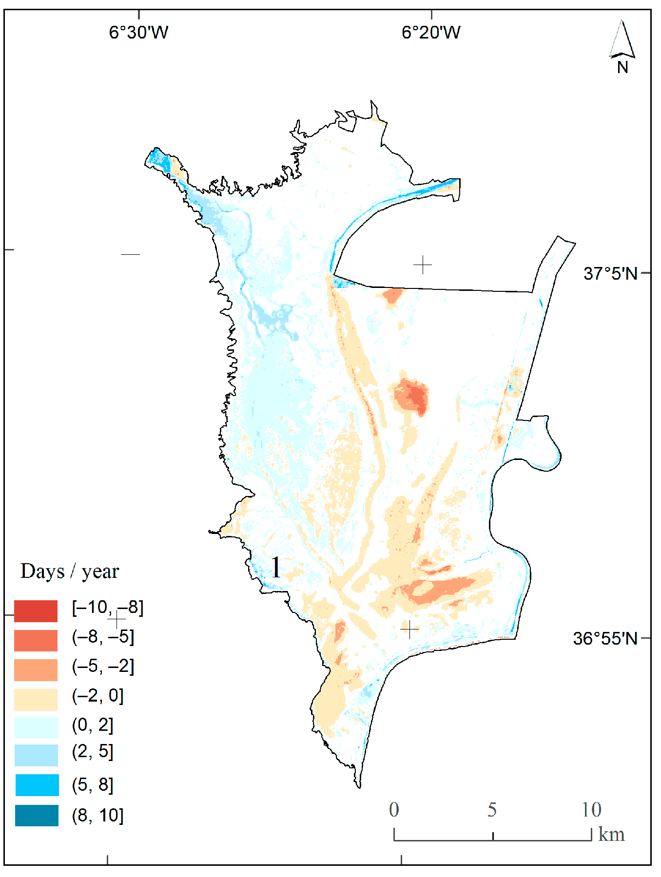
an area (bluish colours in Figure 8) fed by tributaries, both canalized and natural (Caño Travieso, Caño Guadiamar, Arroyo de la Rocina see Figure 1), pumping stations (Lucio de la FAO, label 2 in Figure 7a), groundwater seepages (Lucio del Hondón and Vera Sur labelled as 1 in Figure 8) or brackish waters from Guadalquivir River; and
(b)
a region (reddish colours in Figure 8) strictly fed by rainfall and eventually drained under management decisions for the avoidance of harmful algal blooms [73].

4. Discussion

4.1. Overall Assessment of the Method

Flooding patterns in the Doñana shallow marshes have been retrospectively mapped by means of Landsat imagery. The semiautomatic methodology based on simple threshold in the SWIR band was the most accurate method not only for single dates but also for the whole multi-sensor time series of images. Pre-processing with geometric co-registration and normalization of the Landsat time series proved to be essential to provide consistency to the results [51,57]. A simple threshold on the SWIR band performed accurately across sensors, dates, and marsh conditions. The method worked acceptably with turbid waters as well. Turbidity may eventually reach values of ca. 600 NTU in Doñana marshes. During such episodes flooding was successfully discriminated too. Similar results were observed for flooded pixels densely covered by emergent vegetation. For a few scenes (<1%), errors have been found for areas shadowed by small clouds over the marsh. Cloud masking provided accurate removal of pixels covered by clouds but not cloud shadows. The method is being updated for Landsat 8 OLI and Sentinel-2 images in order to extend the time series of flooding masks and hydroperiods. Microwave sensors such as Sentinel-1 are going to be explored, seeking for an enhancement of hydroperiod estimates by incorporating information for cloud-covered scenes.
While most of the remote sensing applications for wetlands have focused on delineating surface water extent or retrieving water levels [17], few of them have provided insights into hydroperiod mapping. Although optical winter images in the area are influenced by cloud cover—especially in rainy years and winter, images are more problematic due to the low sun angle and shadows—the Doñana hydroperiod estimated from the Landsat time series has been shown to be consistent with in situ observations at limnimetric scales.

4.2. Monitoring Flooding Regime of Doñana Marshes: The Scientific Contribution

The analyzed time span of 40 years adequately represents the immense rainfall variability in Doñana marshes (169 mm in the 2004–2005 cycle; 1032 mm in the cycle 1995–1996; mean rainfall of 550 mm). Rainfall is confirmed as the main driver of the flooding regime in the Doñana marshes. The almost complete isolation from the Guadalquivir estuary before the time series began gives the marshes its endorheic character. Topographical features such as depressions and water courses keep flooding for longer, but sediment transport and siltation dynamics, especially the deposition in the marshes of sandy sediments from tributary ravines, are continuously shaping the marsh bottom [72,74]. The effects of such alterations are evidenced by the synoptic outputs from our analysis.
The rainfall regime over the last 36 years shows no significant trend, with 20 cycles below and 17 above the mean total cycle rainfall. Detailed analysis of management periods shows critical cut-offs, from which the cycles 1983–1984 and 1998–1999 represent subtle shifts towards slight hydroperiod increase (Figure 6). For both dates, management actions were focused on the construction and prolongation of an artificial levee along the Guadalquivir river bank (the so-called Montaña del Río). Restoration actions by the Project Doñana 2005 have been assessed using this valuable information [74]. The deposition rate at the mouth of the El Partido ravine has declined in the last years as a consequence of the upstream dam control. However, the dramatic shift produced in the main water course is evidenced by the hydroperiod increase observed downstream (Figure 7b label 4). The adaptive restoration action in the Caracoles area (Figure 7b label 5), consisting of the creation of artificial ponds and profiling of one tidal course (Caño Travieso), is being revealed by the reconstructed hydroperiod patterns. Nowadays, the restoration program has just implemented the major decision of re-connecting the marsh with the Guadalquivir estuary and with the most relevant tributary to the marsh (the Guadiamar ravine; see Figure 1). The follow-up application of this methodology will enable us to identify early trends as a consequence of such management actions.
The ecological implications of the observed flooding regime are likely visible in the aquatic plant distribution and the habitats available for the waterfowl of Doñana marshes. The flooding gradient has been identified as a major driver for the distribution of emergent helophytes and submerged macrophytes [75]. Submerged macrophytes do play a major role in the marsh metabolism [38]. Hydroperiod becomes a net predictor for aquatic plant species distribution, marsh primary production, and habitat characteristics. Several works have already identified the importance of the hydroperiod duration in predicting the presence, abundance, and breeding success of different waterbird species in the Doñana marshes [76,77,78,79,80,81], and also on raptors foraging in the marshes [82]. The output layers for every single date, i.e., flooding masks and hydroperiod maps per cycle, are accessible online via Web Map Services [83].

5. Conclusions

A semiautomatic procedure to delineate the flooded surface of the Doñana marshes for the last 40 years has provided accurate results sufficient for assessing hydroperiod trends. Time series of Landsat images were standardized to produce consistent flooding masks. Amid different classifiers, a classification tree was found to be the most accurate, using a set of Landsat acquisitions and ground-truth data. The inter-scene cross-validation provided a single optimal threshold for the Landsat TM/ETM+ 5 band and Landsat MSS 4 band. A direct method to estimate the flooding cycle hydroperiod in Doñana marshes has been proposed and tested, providing consistent hydroperiod estimates and revealing a flooding regime mainly driven by rainfall, topography, and local hydrological management actions. Historical trend was assessed by time series analysis, depicting two opposite patterns in the hydroperiod of the Doñana marshes: a significant decrease in the southern area and an increase in the northwestern region. Flooding anomalies are periodically calculated per flooding cycle, allowing us to synoptically assess management decisions and climatic variability and monitor hydrological effects on marsh functioning. Several studies have revealed the utility of the produced spatial layers in predicting changes in associated flora and fauna, also useful for conservation management and restoration programs. The proposed semiautomatic procedure can easily be replicated for other shallow seasonal wetlands.

Supplementary Materials

The following are available online at www.mdpi.com/2072-4292/8/9/775/s1, Figure S1: Location of limnimetric scales in Doñana marshes and water level readings. (A) Location of limnimetric scales in Doñana marshes (red dots). Yellow dots are the ones selected for the plot S2C. Black lines depict the limits of Doñana protected area; (B) Location of Doñana in Spain; (C) Water level readings above sea level (a.s.l.) during the 2003–2004 flooding cycle of the yellow dotted scales in Figure S2A. Table S1: Ground-truth data and training scenes used.

Acknowledgments

This study was funded by the Spanish Ministry of Science and Innovation through the research projects HYDRA (#CGL2006-02247/BOS) and HYDRA2 (CGL2009-09801/BOS), and by funding from the European Union’s Horizon 2020 research and innovation program under grant agreement No. 641762 to ECOPOTENTIAL project. The Espacio Natural de Doñana provided permits for fieldwork in protected areas with restricted access and historical data from water column readings. We are grateful to many MSc students who helped in image processing and field sampling.

Author Contributions

The authors are all intellectually responsible for the conducted research. Ricardo Díaz-Delgado and Javier Bustamante designed the work presented and Ricardo Díaz-Delgado prepared the manuscript. Together with David Aragonés and Isabel Afán, they developed and tested the methodology, processed and analyzed the time series of images, and participated in ground-truth data collection.

Conflicts of Interest

The authors declare no conflict of interest.

References

  1. Garcia Novo, F.; Alonso Vizcaino, E.M.; Marin Cabrera, C. Doñana-Water and Biosphere; Mateu Cromo Artes Gráficas: Madrid, España, 2006. [Google Scholar]
  2. Manzano, M.; Custodio, E.; Mediavilla, C.; Montes, C. Effects of localised intensive aquifer exploitation on the Doñana wetlands (SW Spain). In Groundwater Intensive Use; IAH Selected Papers on Hydrogeology; Taylor & Francis: Leiden, The Netherlands, 2005; p. 401. [Google Scholar]
  3. Casado, S.; Montes, C. Estado de conservación de los humedales peninsulares españoles. Quercus 1991, 66, 18–26. [Google Scholar]
  4. Sánchez Navarro, R. Environmental Flows in the Marsh of the National Park of Doñana and Its Area of Influence; WWF España: Madrid, España, 2009. [Google Scholar]
  5. Méndez, P.F.; Isendahl, N.; Amezaga, J.M.; Santamaría, L. Facilitating Transitional Processes in Rigid Institutional Regimes for Water Management and Wetland Conservation: Experience from the Guadalquivir Estuary. Ecol. Soc. 2012, 17, 26. [Google Scholar] [CrossRef]
  6. Nuttle, W.K. Measurement of wetland hydroperiod using harmonic analysis. Wetlands 1997, 17, 82–89. [Google Scholar] [CrossRef]
  7. Alcorlo, P.; Jimenez, S.; Baltanas, A.; Rico, E. Assessing the patterns of the invertebrate community in the marshes of Donana National Park (SW Spain) in relation to environmental factors. Limnetica 2014, 33, 189–204. [Google Scholar]
  8. Tarr, M.; Babbitt, K.J. The Importance of Hydroperiod in Wetland Assessment A Guide for Community Officials, Planners, and Natural Resource Professionals; University of New Hampshire Cooperative Extension, the UNH Department of Natural Resources, and the NH Fish and Game Department: Durham, NH, USA, 2008. [Google Scholar]
  9. Zhang, M.; Ustin, S.L.; Rejmankova, E.; Sanderson, E.W. Monitoring Pacific coast salt marshes using remote sensing. Ecol. Appl. 1997, 7, 1039–1053. [Google Scholar] [CrossRef]
  10. Baker, C.; Lawrence, R.; Montagne, C.; Patten, D. Mapping wetlands and riparian areas using Landsat ETM+ imagery and decision-tree-based models. Wetlands 2006, 26, 465–474. [Google Scholar] [CrossRef]
  11. Xu, H. Modification of normalised difference water index (NDWI) to enhance open water features in remotely sensed imagery. Int. J. Remote Sens. 2006, 27, 3025–3033. [Google Scholar] [CrossRef]
  12. Belluco, E.; Camuffo, M.; Ferrari, S.; Modenese, L.; Silvestri, S.; Marani, A.; Marani, M. Mapping salt-marsh vegetation by multispectral and hyperspectral remote sensing. Remote Sens. Environ. 2006, 105, 54–67. [Google Scholar] [CrossRef]
  13. Cózar, A.; García, C.M.; Gálvez, J.A.; Loiselle, S.A.; Bracchini, L.; Cognetta, A. Remote sensing imagery analysis of the lacustrine system of Ibera wetland (Argentina). Ecol. Model. 2005, 186, 29–41. [Google Scholar] [CrossRef]
  14. Doxaran, D.; Castaing, P.; Lavender, S.J. Monitoring the maximum turbidity zone and detecting fine-scale turbidity features in the Gironde estuary using high spatial resolution satellite sensor (SPOT HRV, Landsat ETM+) data. Int. J. Remote Sens. 2006, 27, 2303–2321. [Google Scholar] [CrossRef]
  15. Lira, J. Segmentation and morphology of open water bodies from multispectral images. Int. J. Remote Sens. 2006, 27, 4015–4038. [Google Scholar] [CrossRef]
  16. Shanmugam, P.; Ahn, Y.H.; Sanjeevi, S. A comparison of the classification of wetland characteristics by linear spectral mixture modelling and traditional hard classifiers on multispectral remotely sensed imagery in southern India. Ecol. Model. 2006, 194, 379–394. [Google Scholar] [CrossRef]
  17. Gardiner, N.; Díaz-Delgado, R. Trends in Selected Biomes, Habitats and Ecosystems: Inland Waters. In Sourcebook on Remote Sensing and Biodiversity Indicators; Technical Series; Secretariat of the Convention on Biological Diversity: Montreal, QC, Canada, 2007; pp. 83–102. [Google Scholar]
  18. Davranche, A.; Poulin, B.; Lefebvre, G. Mapping flooding regimes in Camargue wetlands using seasonal multispectral data. Remote Sens. Environ. 2013, 138, 165–171. [Google Scholar] [CrossRef] [Green Version]
  19. Jain, S.K.; Singh, R.D.; Jain, M.K.; Lohani, A.K. Delineation of Flood-Prone Areas Using Remote Sensing Techniques. Water Resour. Manag. 2005, 19, 333–347. [Google Scholar] [CrossRef]
  20. Overton, I.C. Modelling floodplain inundation on a regulated river: integrating GIS, remote sensing and hydrological models. River Res. Appl. 2005, 21, 991–1001. [Google Scholar] [CrossRef]
  21. Johnston, R.; Barson, M. Remote sensing of Australian wetlands: An evaluation of Landsat TM data for inventory and classification. Mar. Freshw. Res. 1993, 44, 235–252. [Google Scholar] [CrossRef]
  22. Bustamante, J.; Pacios, F.; Díaz-Delgado, R.; Aragonés, D. Predictive models of turbidity and water depth in the Doñana marshes using Landsat TM and ETM+ images. J. Environ. Manage. 2009, 90, 2219–2225. [Google Scholar] [CrossRef] [PubMed]
  23. Binding, C.E.; Bowers, D.G.; Mitchelson-Jacob, E.G. Estimating suspended sediment concentrations from ocean colour measurements in moderately turbid waters; the impact of variable particle scattering properties. Remote Sens. Environ. 2005, 94, 373–383. [Google Scholar] [CrossRef]
  24. Marti-Cardona, B.; Dolz-Ripolles, J.; Lopez-Martinez, C. Wetland inundation monitoring by the synergistic use of ENVISAT/ASAR imagery and ancilliary spatial data. Remote Sens. Environ. 2013, 139, 171–184. [Google Scholar] [CrossRef]
  25. Ramos-Fuertes, A.; Marti-Cardona, B.; Blade, E.; Dolz, J. Envisat/ASAR Images for the Calibration of Wind Drag Action in the Donana Wetlands 2D Hydrodynamic Model. Remote Sens. 2014, 6, 379–406. [Google Scholar] [CrossRef] [Green Version]
  26. Marti-Cardona, B.; Lopez-Martinez, C.; Dolz-Ripolles, J.; Bladè-Castellet, E. ASAR polarimetric, multi-incidence angle and multitemporal characterization of Doñana wetlands for flood extent monitoring. Remote Sens. Environ. 2010, 114, 2802–2815. [Google Scholar] [CrossRef]
  27. Bourgeau-Chavez, L.; Endres, S.; Battaglia, M.; Miller, M.E.; Banda, E.; Laubach, Z.; Higman, P.; Chow-Fraser, P.; Marcaccio, J. Development of a bi-national great lakes coastal wetland and land use map using three-season PALSAR and Landsat imagery. Remote Sens. 2015, 7, 8655–8682. [Google Scholar] [CrossRef]
  28. Bourgeau-Chavez, L.L.; Smith, K.B.; Brunzell, S.M.; Kasischke, E.S.; Romanowicz, E.A.; Richardson, C.J. Remote monitoring of regional inundation patterns and hydroperiod in the Greater Everglades using Synthetic Aperture Radar. Wetlands 2005, 25, 176–191. [Google Scholar] [CrossRef]
  29. Hong, S.H.; Kim, H.O.; Wdowinski, S.; Feliciano, E. Evaluation of polarimetric SAR decomposition for classifying wetland vegetation types. Remote Sens. 2015, 7, 8563–8585. [Google Scholar] [CrossRef]
  30. Lyon, J.G.; Lyon, L.K. Practical Handbook for Wetland Identification and Delineation, Second Edition; CRC Press: Boca Raton, FL, USA, 2011. [Google Scholar]
  31. White, L.; Brisco, B.; Dabboor, M.; Schmitt, A.; Pratt, A. A collection of SAR methodologies for monitoring wetlands. Remote Sens. 2015, 7, 7615–7645. [Google Scholar] [CrossRef]
  32. Röder, A.; Kuemmerle, T.; Hill, J. Extension of retrospective datasets using multiple sensors. An approach to radiometric intercalibration of Landsat TM and MSS data. Remote Sens. Environ. 2005, 95, 195–210. [Google Scholar] [CrossRef]
  33. Wang, Z.; Zhang, B.; Zhang, S.; Li, X.; Liu, D.; Song, K.; Li, J.; Li, F.; Duan, H. Changes of land use and of ecosystem service values in Sanjiang Plain, Northeast China. Environ. Monit. Assess. 2006, 112, 69–91. [Google Scholar] [CrossRef] [PubMed]
  34. Lan, Z.; Zhang, D. Study on optimization-based layered classification for separation of wetlands. Int. J. Remote Sens. 2006, 27, 1511–1520. [Google Scholar] [CrossRef]
  35. Leimgruber, P.; Christen, C.A.; Laborderie, A. The impact of landsat satellite monitoring on conservation biology. Environ. Monit. Assess. 2005, 106, 81–101. [Google Scholar] [CrossRef] [PubMed]
  36. Islam, M.A.; Thenkabail, P.S.; Kulawardhana, R.W.; Alankara, R.; Gunasinghe, S.; Edussriya, C.; Gunawardana, A. Semi-automated methods for mapping wetlands using Landsat ETM+ and SRTM data. Int. J. Remote Sens. 2008, 29, 7077–7106. [Google Scholar] [CrossRef]
  37. Haberl, H.; Gaube, V.; Díaz-Delgado, R.; Krauze, K.; Neuner, A.; Peterseil, J.; Plutzar, C.; Singh, S.J.; Vadineanu, A. Towards an integrated model of socioeconomic biodiversity drivers, pressures and impacts. A feasibility study based on three European long-term socio-ecological research platforms. Ecol. Econ. 2009, 68, 1797–1812. [Google Scholar] [CrossRef] [Green Version]
  38. Duarte, C.; Montes, C.; Agustí, S.; Martino, P.; Bernués, M.; Kalff, J. Biomasa de macrófitos acuáticos en la marisma del Parque Nacional de Doñana (SW España): Importancia y factores ambientales que controlan su distribución. Limnetica 1990, 6, 1–12. [Google Scholar]
  39. Díaz-Delgado, R. La investigación y seguimiento ecológico a largo plazo (LTER). Ecosistemas 2016, 25, 1–3. [Google Scholar] [CrossRef]
  40. Hall, F.G.; Strebel, D.E.; Nickeson, J.E.; Goetz, S.J. Radiometric rectification: Toward a common radiometric response among multidate, multisensor images. Remote Sens. Environ. 1991, 35, 11–27. [Google Scholar] [CrossRef]
  41. Schott, J.R.; Salvaggio, C.; Volchok, W.J. Radiometric scene normalization using pseudoinvariant features. Remote Sens. Environ. 1988, 26, 1–16. [Google Scholar] [CrossRef]
  42. De Junta, A. Ortofotografía digital de Andalucía (color) 1998–1999. Cons. Obras Públ. Transp. 2003. [Google Scholar]
  43. Chuvieco, E. Teledetección ambiental: La observación de la tierra desde el espacio, 3rd ed.; Ariel: Barcelona, Spain, 2010. [Google Scholar]
  44. Maxwell, S.K.; Schmidt, G.L.; Storey, J.C. A multi-scale segmentation approach to filling gaps in Landsat ETM+ SLC-off images. Int. J. Remote Sens. 2007, 28, 5339–5356. [Google Scholar] [CrossRef]
  45. Chen, J.; Zhu, X.; Vogelmann, J.E.; Gao, F.; Jin, S. A simple and effective method for filling gaps in Landsat ETM+ SLC-off images. Remote Sens. Environ. 2011, 115, 1053–1064. [Google Scholar] [CrossRef]
  46. Pons, X.; Solé-Sugrañes, L. A simple radiometric correction model to improve automatic mapping of vegetation from multispectral satellite data. Remote Sens. Environ. 1994, 48, 191–204. [Google Scholar] [CrossRef]
  47. Chavez, P.S. Image-based atmospheric corrections-revisited and improved. Photogramm. Eng. Remote Sens. 1996, 62, 1025–1035. [Google Scholar]
  48. McGovern, E.A.; Holden, N.M.; Ward, S.M.; Collins, J.F. The radiometric normalization of multitemporal Thematic Mapper imagery of the midlands of Ireland-a case study. Int. J. Remote Sens. 2002, 23, 751–766. [Google Scholar] [CrossRef]
  49. Pons, X.; Pesquer, L.; Cristóbal, J.; González-Guerrero, O. Automatic and improved radiometric correction of landsat imageryusing reference values from MODIS surface reflectance images. Int. J. Appl. Earth Obs. Geoinf. 2014, 33, 243–254. [Google Scholar] [CrossRef]
  50. Díaz-Delgado, R.; Bustamante, J.; Aragonés, D.; Pacios, F. Determining water body characteristics of Doñana shallow marshes through remote sensing. In Proceedings of the International Geoscience and Remote Sensing Symposium, Denver, CO, USA, 2006.
  51. Díaz-Delgado, R.; Aragonés, D.; Ameztoy, I.; Bustamante, J. Monitoring marsh dynamics through remote sensing. In Conservation Monitoring in Freshwater Habitats; Hurford, C., Scheneider, M., Cowx, I., Eds.; Springer: New York, NY, USA, 2010; pp. 375–386. [Google Scholar]
  52. Bilge, F.; Yazici, B.; Dogeroglu, T.; Ayday, C. Statistical evaluation of remotely sensed data for water quality monitoring. Int. J. Remote Sens. 2003, 24, 5317–5326. [Google Scholar] [CrossRef]
  53. Montesinos, S.; Castaño, S.M. Monitoring of Wetlands Evolution; European Comission: Madrid, España, 1999. [Google Scholar]
  54. Domínguez Gómez, J.A. Estudio de la Calidad del Agua de Lagunas de Gravera Mediante Teledetección. Ph.D. Thesis, Universidad de Alcalá de Henares, Alcalá de Henares, Madrid, 2003. [Google Scholar]
  55. Ordoyne, C.; Friedl, M.A. Using MODIS data to characterize seasonal inundation patterns in the Florida Everglades. Remote Sens. Environ. 2008, 112, 4107–4119. [Google Scholar] [CrossRef]
  56. Kyu-Shun, L.K.; Yeo-Sang, Y.; Sang-Ming, S. Spectral characteristics of shallow turbid water near the shoreline on in ter-tidal flat. Korean J. Remote Sens. 2001, 17, 131–139. [Google Scholar]
  57. Bustamante, J.; Díaz-Delgado, R.; Aragonés, D. Determinación de las características de masas de aguas someras en las marismas de Doñana mediante teledetección. Rev. Teledetec. 2005, 24, 107–111. [Google Scholar]
  58. Cohen, J. A Coefficient of agreement for nominal scales. Educ. Psychol. Meas. 1960, 20, 37–46. [Google Scholar] [CrossRef]
  59. Lillesand, T. Remote Sensing and Image Interpretation, 6th Revised Edition; Wiley: Hoboken, NJ, USA, 2008. [Google Scholar]
  60. Pradhan, B. Remote sensing and GIS-based landslide hazard analysis and cross-validation using multivariate logistic regression model on three test areas in Malaysia. Adv. Space Res. 2010, 45, 1244–1256. [Google Scholar] [CrossRef]
  61. Foody, G.M.; Mathur, A. A relative evaluation of multiclass image classification by support vector machines. IEEE Trans. Geosci. Remote Sens. 2004, 42, 1335–1343. [Google Scholar] [CrossRef]
  62. Díaz-Delgado, R.; Lloret, F.; Pons, X. Spatial patterns of fire occurrence in Catalonia, NE, Spain. Landsc. Ecol. 2004, 19, 731–745. [Google Scholar] [CrossRef]
  63. Hoaglin, D.C.; Mosteller, F.; Tukey, J.W. Understanding Robust and Exploratory Data Analysis; John Wiley & Sons: New York, NY, USA, 2000. [Google Scholar]
  64. Anyamba, A.; Tucker, J.C.; Eastman, J.R. NDVI anomaly patterns over Africa during the 1997/98 ENSO warm event. Int. J. Remote Sens. 2001, 22, 1847–1859. [Google Scholar]
  65. Fernández-Delgado, C. Doñana fish species threats affecting a community in decline. In Doñana, Water and Biosphere; Confederación Hidrográfica del Guadalquivir. Ministerio de Medio Ambiente: Madrid, España, 2006; pp. 237–242. [Google Scholar]
  66. Ibáñez, E.; Gili, J.A.; Ripollès, J.D.; Bayán, B. MDT de precisión de la marisma del P.N. de Doñana mediante láser escáner aerotransportado (LIDAR). Rev. Inst. Naveg. Esp. Publ. Téc. Cuatrimest. Naveg. Marítima Aérea Espac. Terr. 2007, 14–25. [Google Scholar]
  67. Frisch, D.; Moreno-Ostos, E.; Green, A.J. Species richness and distribution of copepods and cladocerans and their relation to hydroperiod and other environmental variables in Doñana, south-west Spain. Hydrobiologia 2006, 556, 327–340. [Google Scholar] [CrossRef]
  68. Frisch, D.; Rodríguez-Pérez, H.; Green, A.J. Invasion of artificial ponds in Doñana Natural Park, southwest Spain, by an exotic estuarine copepod. Aquat. Conserv. Mar. Freshw. Ecosyst. 2006, 16, 483–492. [Google Scholar] [CrossRef]
  69. Santamaría, L.; Green, A.; Díaz-Delgado, R.; Bravo, M.Á.; Castellanos, E. Caracoles: A new laboratory for science and wetland restoration. In Doñana, Water and Biosphere; Confederación Hidrográfica del Guadalquivir. Ministerio de Medio Ambiente: Madrid, España, 2006; pp. 313–315. [Google Scholar]
  70. Sebastián-González, E.; Green, A.J. Reduction of avian diversity in created versus natural and restored wetlands. Ecography 2016, in press. [Google Scholar]
  71. Equipo de Seguimiento de Doñana; ICTS-Reserva Biológica de Doñana (EBD-CSIC). Memoria del año hidrometeorológico 2007–2008. Programa de Seguimiento de Procesos y Recursos Naturales en el Espacio Natural Doñana; Dirección General de Espacios Naturales y Participación Ciudadana. Junta de Andalucía—Estación Biológica de Doñana (CSIC): Sevilla, España, 2008; p. 199. [Google Scholar]
  72. García-Novo, F.; García, J.C.E.; Carotenuto, L.; Sevilla, D.G.; Faso, R.P.F.L. The restoration of El Partido stream watershed (Doñana Natural Park): A multiscale, interdisciplinary approach. Ecol. Eng. 2007, 30, 122–130. [Google Scholar] [CrossRef]
  73. Báez, J.C.; Real, R.; López-Rodas, V.; Costas, E.; Salvo, A.E.; García-Soto, C.; Flores-Moya, A. The North Atlantic Oscillation and the Arctic Oscillation favour harmful algal blooms in SW Europe. Harmful Algae 2014, 39, 121–126. [Google Scholar] [CrossRef]
  74. Chans, J.J.; Díaz-Delgado, R. Monitoring and Evaluation: The key to the Doñana 2005 Restoration Project. In Doñana, Water and Biosphere; Confederación Hidrográfica del Guadalquivir. Ministerio de Medio Ambiente: Madrid, España, 2006; pp. 319–326. [Google Scholar]
  75. Espinar, J.L.; García, L.V.; García Murillo, P.; Toja, J. Submerged macrophyte zonation in a Mediterranean salt marsh: A facilitation effect from established helophytes? J. Veg. Sci. 2002, 13, 831–840. [Google Scholar] [CrossRef]
  76. Kloskowski, J.; Green, A.J.; Polak, M.; Bustamante, J.; Krogulec, J. Complementary use of natural and artificial wetlands by waterbirds wintering in Doñana, south-west Spain. Aquat. Conserv. Mar. Freshw. Ecosyst. 2009, 19, 815–826. [Google Scholar] [CrossRef]
  77. Ramo, C.; Aguilera, E.; Figuerola, J.; Máñez, M.; Green, A.J. Long-term population trends of colonial wading birds breeding in Doñana (SW Spain) in relation to environmental and anthropogenic factors. Ardeola 2013, 60, 305–326. [Google Scholar] [CrossRef]
  78. Márquez-Ferrando, R.; Figuerola, J.; Hooijmeijer, J.C.E.W.; Piersma, T. Recently created man-made habitats in Doñana provide alternative wintering space for the threatened Continental European black-tailed godwit population. Biol. Conserv. 2014, 171, 127–135. [Google Scholar] [CrossRef]
  79. Toral, G.M.; Aragonés, D.; Bustamante, J.; Figuerola, J. Using Landsat images to map habitat availability for waterbirds in rice fields. Ibis 2011, 153, 684–694. [Google Scholar] [CrossRef]
  80. Rendón, M.A.; Green, A.J.; Aguilera, E.; Almaraz, P. Status, distribution and long-term changes in the waterbird community wintering in Doñana, south–west Spain. Biol. Conserv. 2008, 141, 1371–1388. [Google Scholar] [CrossRef] [Green Version]
  81. Ramírez, F.; Navarro, J.; Afán, I.; Hobson, K.A.; Delgado, A.; Forero, M.G. Adapting to a changing world: Unraveling the role of man-made habitats as alternative feeding areas for slender-billed gull (Chroicocephalus genei). PLoS ONE 2012, 7. [Google Scholar] [CrossRef] [Green Version]
  82. Sergio, F.; Blas, J.; López, L.; Tanferna, A.; Díaz-Delgado, R.; Donázar, J.A.; Hiraldo, F. Coping with uncertainty: Breeding adjustments to an unpredictable environment in an opportunistic raptor. Oecologia 2011, 166, 79–90. [Google Scholar] [CrossRef] [PubMed]
  83. Díaz-Delgado, R. Servidor de Imágenes Landsat y productos derivados de Doñana. Available online: http://venus.ebd.csic.es/imgs/ (accessed on 15 September 2016).
Figure 1. Location of (a) Andalusia in Europe and (b) Doñana in Andalusia at the mouth of the Guadalquivir River; (c) the area covered by Doñana natural marshes (solid blue) within the protected area of Doñana National and Natural parks (red line). Numbers indicate main tributary rivers and ravines (1. Arroyo de la Rocina; 2. Arroyo del Partido; 3. Encauzamiento del Río Guadiamar). Background: False color composite of a 2007 Landsat TM image.
Remotesensing 08 00775 g001
Figure 2. Different flooding features in Doñana marshes showing the spatio-temporal variability found in these wetlands. The flooded picture shows the shallow inundation with variable plant cover and turbidity.
Remotesensing 08 00775 g002
Figure 3. Flowchart of the methodology followed in the study.
Remotesensing 08 00775 g003
Figure 4. (a) Overlay of flooding masks for the wet cycle in 2003–2004 (total rainfall = 775 mm); (b) calculated hydroperiod in number of days for the same cycle. Color palettes and number of classes are the same for comparison purposes. The white tack indicates the location of the N28 limnimetric scale.
Remotesensing 08 00775 g004
Figure 5. Number of total available flooding masks per flooding cycle. Gini coefficients are also depicted (solid line), pointing up the uniform distribution of flooding masks for every flooding cycle (high values indicate uneven distribution of available flooding masks). Cycle range values are also shown (dotted line), revealing the time span between the earliest and latest flooding masks. Asterisks indicate the discarded cycles for time series analysis.
Remotesensing 08 00775 g005
Figure 6. Mean marsh hydroperiod versus total accumulated rainfall per flooding cycle. Asterisks indicate the discarded cycles for time series analysis. Rainfall data available since 1978.
Remotesensing 08 00775 g006
Figure 7. (a) Mean hydroperiod for Doñana marshes (1974–2014); (b) Hydroperiod anomaly calculated for the flooding cycle 2007–2008. Both are expressed in days per year. Numbers in both figures indicate interesting features (see text for more details).
Remotesensing 08 00775 g007
Figure 8. Theil–Sen slope in days/year for the hydroperiod time series (1974–2014). Red indicates consistent and significant decreasing trend while blue indicates the opposite. Yellowish pixels show significant but slight trends. Transparent pixels show non-significant trends. Label 1 locates Vera Sur (see text for details).
Remotesensing 08 00775 g008
Table 1. Ground-truth points collected variables with their corresponding units and categories.
VariableUnitsCategories/Range
TurbidityNefelometric Turbid Units (NTU)Continuous (0–653)
Water DepthCentimeterContinuous (0–140)
Water conductivitymicroSiemens/cm2Continuous (300–42,700)
Dry bare-ground coverPercent per pixel0%, 1%–5%, 5%–25%, 25%–75%, >75%
Plant typePlant dominant speciesEmergent, floating, submerged, algae
Plant statusAlive/Dead% Green/% Dry
Plant cover per plant typePercent per pixel0%, 1%–5%, 5%–25%, 25%%–75%, >75%
Alien spp abundancePercent per pixel0%, 1%–5%, 5%–25%, 25%–50%, 50%–75%, >75%
Open waterPercent per pixel0%, 1%–5%, 5%–25%, 25%–75%, >75%
Flood coverPercent per pixel0%, 1%–5%, 5%–25%, 25%–75%, >75%
Table 2. Mean overall agreement values and mean Kappa values for the five classification methods compared for the classes flooded and non-flooded. Standard deviation is shown in brackets. Statistics are from the eight Landsat training scenes.
MethodMean AccuracyMean Kappa
Maximum Likelihood0.78 (0.14)0.50 (0.23)
Mahalanobis Distance0.80 (0.13)0.55 (0.23)
Discriminant Analysis0.84 (0.07)0.62 (0.16)
Logistic Regression0.85 (0.06)0.61 (0.16)
Classification Tree0.85 (0.06)0.64 (0.14)
Table 3. Band 5 reflectance thresholds estimated from classification trees on the set of training Landsat images. Kappa and global accuracy values for every classification tree are also provided. Dates in the first column indicate the discarded scene for every cross-validation model. The total number of ground-truth points (N) used for validation is also shown.
Discarded Scene Modelsρ ThresholdGlobal AccuracyKappaN
25 March 20040.1880.9550.429112
11 February 20060.1850.9800.91250
8 April 20060.1840.9800.87850
2 May 20060.1820.9810.92253
3 June 20060.1890.8580.325122
10 November 20060.1800.9460.81793
2 March 20070.1900.9280.418138
18 March 20070.1840.9140.560160
All scenes model0.1860.9330.605778

