Multi-Task Joint Sparse and Low-Rank Representation for the Scene Classification of High-Resolution Remote Sensing Image

Abstract

Scene classification plays an important role in the intelligent processing of High-Resolution Satellite (HRS) remotely sensed images. In HRS image classification, multiple features, e.g., shape, color, and texture features, are employed to represent scenes from different perspectives. Accordingly, effective integration of multiple features always results in better performance compared to methods based on a single feature in the interpretation of HRS images. In this paper, we introduce a multi-task joint sparse and low-rank representation model to combine the strength of multiple features for HRS image interpretation. Specifically, a multi-task learning formulation is applied to simultaneously consider sparse and low-rank structures across multiple tasks. The proposed model is optimized as a non-smooth convex optimization problem using an accelerated proximal gradient method. Experiments on two public scene classification datasets demonstrate that the proposed method achieves remarkable performance and improves upon the state-of-art methods in respective applications.

1. Introduction

With the rapid development of remote sensing techniques over recent years, High-Resolution Satellite (HRS) images are becoming increasingly available thus enabling us to study earth observations in greater detail. However, despite enhanced resolution, these details often suffer from the spectral uncertainty problem stemming from an increase of the intra-class variance and decrease of the inter-class variance [1], and the curse of dimensionality problem resulting from the small ratio between the number of training samples and features [2]. Taking into account these characteristics, HRS image classification methods have evolved from pixel-oriented methods to object-oriented methods and achieved precise object recognition [3,4,5]. Object-oriented feature extraction methods cluster homogeneous pixels and take advantage of both local and global properties [6]. These successful developments in feature extraction technologies for HRS satellite images have increased the usefulness of remote sensing applications in environmental and land resource management, security and defense issues, and urban planning, etc.

Scene representation and recognition of HRS satellite images is a challenging task given the ambiguity and variability of scenes, and has attracted much attention in recent years [7,8,9,10]. Scene classification is aimed at automatically labeling an image from a set of semantic categories [11,12,13]. In this paper, the term “scenes” refers to separated sub-blocks split from a large satellite image. Scenes often contain multiple land-cover objects having a specific semantic meaning, such as an agricultural area, residential area, mobile home park, and golf course in a satellite image. These high-level latent semantic concepts make it difficult to recognize HRS satellite scenes. As a consequence, the main problem in the HRS satellite scene interpretation is bridging semantic gaps [14]. Semantic-based scene classification has been widely applied in HRS image scene interpretation [15,16]. It is usually difficult to understand and recognize scene categories because of the high complexity of spatial and structural patterns in the massive HRS satellite images [17]. Therefore, feature representation in each scene is a key step and highly demanded for accurate scene classification.

To obtain the meaningful features for scene classification, many descriptors have been developed in recent years. Features such as color distributions describing the reflective spectral information [18,19], textures reflecting a specific and spatially repetitive pattern of surfaces [20,21], and structures containing macroscopic relationships between objects [22,23] have been widely used in HRS satellite image classification; however, none of the feature descriptors has the same discriminating power for all classes of scenes. For example, features based on color information might perform well when classifying forest and desert, while a classifier for residential areas should be invariant to the actual color of the scenes. Therefore, instead of using a single modality of feature for all classes, adaptively fusing a set of diverse and complementary feature modalities might more accurately and precisely discriminate a class from all others.

There are two general fusion strategies within the machine learning trend to semantic scene analysis, namely: early fusion and late fusion. The former combines cues prior to feature extraction [11,24], and the latter first separately extracts features and then combines them at the classifier stage [25,26]. Both early and later fusion methods can be used to classify an HRS image because satellite scene classes have multiple features dependency and independency simultaneously [6,27]. Because different features may have different scales, hard combination methods, such as concatenation, may cause redundancy and degenerate efficiency and performance. Recent studies on Multiple Kernel Learning (MKL) [28] that fuse different features through multiple similarity function combinations can effectively improve the classification performance [29,30]. Several combination methods inspired by MKL have been proposed varying from linear to nonlinear, and from the same type of kernel to different types of kernels [25,31].

In contrast to this family of work, Yuan et al. [32] proposed a Multi-Task Joint Sparse Representation and Classification (MTJSRC) framework for visual recognition in a regularized Multi-Task Learning (MTL) framework. The idea behind MTL is basically that, when the tasks to be learned are similar or related in some sense, it may be advantageous to take into account these cross-task relations in the model. Experimental results have demonstrated the effectiveness of such a framework [33,34]. The MTJSRC framework was motivated by the success of multi-task joint sparse linear regression and the Sparse Representation Classification (SRC) [35] approaches, that have been applied in HRS satellite image classification and achieve excellent performances [36,37]. Based on the knowledge transferring mechanism in MTL [38] and the collaborative representation mechanism in SRC [39], MTJSRC can deal with the “lack of samples” problem for high-dimensional signal recognition [36]. The MTJSRC method can learn a common subset of features for all tasks through joint sparsity regularization [40] by penalizing the sum of $l_2$ norms of the blocks of coefficients associated with each covariate group across different classification problems. From the perspective of linear regression, MTJSRC was inspired by Multi-Task Joint Covariate Selection (MTJCS) which can be regarded as a combination model of the group Least Absolute Shrinkage and Selection Operator (LASSO) [41] and multi-task LASSO [42]. Li et al. [36] introduced the MTJSRC paradigm for hyperspectral image classification and achieved competitive performance. However, the multiple learning tasks in MTJSRC can be coupled using a set of shared factors possessing low-rank structure [43]. For example, satellite scene images with different labels may share similar background under a low-rank structure. Chen et al. [44] demonstrated the effectiveness of the MTL formulation considering the sparse and low-rank patterns from multiple related tasks.

Inspired by the existing works in these fields, we present a Multi-Task Joint Sparse and Low-rank Representation and Classification (MTJSLRC) for HRS images. In this paper, the term “multi-task” means that several linear representation models are simultaneously estimated through regularization on parameters across all the models. For example, when classifying scenes, we obtain K different linear representation models from K different visual features (e.g., texture, shape, and color). The joint sparsity and low-rank structures are enforced by imposing the $l_{1,2}$-norm penalty as proposed by [38,40] and trace norm penalty as previously developed approaches in [45,46]. The objective in MTJSLRC is to determine a squared reconstruction error term and two convex but non-smooth ($l_{1,2}$-norm and trace norm) regularization terms. We deform the model and then use the Accelerated Proximal Gradient (APG) method [47] to solve this non-smooth convex optimization problem. Similar to MTJSRC, classification is ruled in favor of the class that has lowest total reconstruction error accumulated from all the tasks [32]. Extensive experiments show that our method takes advantage of multiple features and thus overcomes the over-fitting problem produced by the hyper-dimensional stacked feature space and “lack of samples.” In our framework, a low-rank constraint is applied to reduce redundancy and correlation in highly correlated tasks for HRS satellite image classification.

The contribution of this study lies in the combination of multiple features based on MTL, SRC, and low-rank representation. We found that the multi-task joint sparse and low-rank representation is a simple yet effective way to combine multiple complementary features to improve the HRS image classification accuracy. We overcome the problem of incoherent sparse and low-rank patterns by considering multiple related features, and decomposing model parameters as a joint sparsity-inducing component and a low-rank component. Specifically, we employ a $l_{1,2}$-norm regularization term to enforce group sparsity in the model parameter, and identify the essential discriminative features for effective HRS image classification; meanwhile, we use a trace-norm constraint to encourage the low-rank structure, capturing the underlying relationship among the tasks for improved generalization performance. We employ the APG method to solve this as a non-smooth convex optimization problem.

The remainder of this paper is organized as follows: Section 2 briefly introduces the basic theory of sparse representation. Section 3 describes the proposed MTJSLRC framework for HRS image classification. The experimental results and analysis are presented in Section 4. In Section 5, some concluding remarks and prospects for future work close the paper.

Notations: For any matrix $\mathrm{X}\in R^{m\times n}$, let $x_{ij}$ be the entry in the $i$-th row and $j$-th column of $\mathrm{X}$; $X^T$ denotes the transpose of $X$; ${\Vert X\Vert }_0$ denotes the $l_0$-norm which counts the number of non-zero entries in $\mathrm{X}$; let ${\Vert X\Vert }_1$ denote the $l_1$-norm and ${\Vert X\Vert }_1={\displaystyle \sum }_{i=1}^m{\displaystyle \sum }_{j=1}^n\left|a_{ij}\right|$; let ${\Vert X\Vert }_F=\sqrt{{\displaystyle \sum }_{i=1}^m{\displaystyle \sum }_{j=1}^n{\left|a_{ij}\right|}^2}$; let ${\Vert X\Vert }_{*}$ denote the nuclear norm which is the sum of absolute value of all the singular values.

2. Related Work

In this section, we briefly review the SRC and MTJSRC methods in scene classification. The working mechanism of the MTJSRC method is depicted in Figure 1. The MTJSRC method can combine a set of diverse and complementary modalities of features to discriminate each class better from all other classes. Instead of extracting multiple feature modalities, the MTJSRC method reduces to the SRC method when using a single modality of feature.

2.1. Sparse Representation Classification

Previous studies have shown that the sparse representation model is discriminative and particularly useful for robust multi-class classification [32]. Assuming that we have $J$ distinct classes, we define $X_j\in R^{d\times n_j}$ as a stack of $n_j$ columns of d-dimension feature vectors from training images labeled as class $j\in \left\{1,\cdots ,J\right\}$, and $\mathrm{n}={{\displaystyle \sum }}_{j=1}^J{n}_j$ Each sub-dictionary $X_j$ can model a convex set for a specific class, and the collaborative dictionary $\mathrm{X}\in R^{d\times n}$, made up of all the sub-dictionary $X_j$, maps each feature vectors into a new dimensional space corresponding to the dictionary. Given a testing image feature $\mathrm{y}\in R^d$, the optimization problem of the sparse linear representation model is described as follows:

$$\widehat{w}=\underset{w}{\min }{\Vert w\Vert }_0,\mathrm{s}.\mathrm{t}.\Vert y-Xw\Vert \le \epsilon ,$$

(1)

where $\epsilon$ denotes the noise level parameter. The problem Equation (1) is NP-hard, but previous research results [48] show that under mild assumptions, this problem can be relaxed as the following objective function:

$$\widehat{w}=\underset{w}{\min }{\Vert w\Vert }_1,\mathrm{s}.\mathrm{t}.\Vert y-Xw\Vert \le \epsilon ,$$

(2)

This optimization problem is convex and the optimal solution $\widehat{w}$ can be efficiently solved. Then, for classification, the class of the image feature $y$ can be determined by minimizing the reconstruction error $r_j$ (error between $y$ and the linearly reconstructed result from the training images in the $j$-th class) as follows:

$$\mathrm{class}\left(\mathrm{y}\right)=\widehat{j}=\underset{j\in \left\{1,\cdots ,J\right\}}{\arg \min }{r}_j\left(y\right)=\underset{j\in \left\{1,\cdots ,J\right\}}{\arg \min }{\Vert y-X_j{\widehat{w}}_j\Vert }^2,$$

(3)

where ${\widehat{w}}_j$ denotes the components of $\widehat{w}$ corresponding to class $j$. In the study of face recognition, the SRC is expressed as the model Equation (2) and the decision rule Equation (3).

2.2. Multi-Task Joint Sparse Representation Classification

The SRC model was originally developed for a single feature, and the MTJSRC model extended it to multiple features and instances-based visual recognition. Suppose K modalities of features for all the training samples with M classes, and the $X^k\in R^{d_k\times n}$ is the training feature matrix for each modality index $k=1,\cdots ,K$. Then, we denote $X_j^k\in R^{d_k\times n_j}$ as the $n_j$ columns of $X^k$ associated with the $j$-th class. For a testing image, let $\mathrm{y}=\left\{y^{kl}\in R^{d_k} k=1,\cdots ,K, l=1,\cdots ,L\right\}$ be the ensemble of L different instances (e.g., multiple transformation of a HRS scene) with same K modalities of features as training images. For each testing image feature $y^{kl}$, we suppose the representation vector as $W^{kl}={[{\left(W_1^{kl}\right)}^T,\cdots ,{\left(W_J^{kl}\right)}^T]}^T$, which $W_j^{kl}\in R^{n_j}$ restricts on class $j$. We define the coefficients associated with class $j$ as $W_j=[W_j^{11},\cdots ,W_j^{KL}]\in R^{n_j\times KL}$. Thus, the multi-task joint covariate selection model in sparse learning [40] seeks to solve the following optimization problem:

$$\widehat{W}=\underset{W}{\arg \min }f\left(W\right)+\mathsf{\alpha }P\left(W\right),$$

(4)

where the expressions of $f\left(W\right)$ and $P\left(W\right)$ are defined respectively as

$$f\left(W\right)=\frac{1}{2}{{\displaystyle \sum }}_{k=1}^K{{\displaystyle \sum }}_{l=1}^L{\Vert y^{kl}-X^k{W}^{kl}\Vert }^2,$$

(5)

$$P\left(W\right)={{\displaystyle \sum }}_{j=1}^J{\Vert W_j\Vert }_F,$$

(6)

This optimized problem can be solved by the APG method [47]. Given the optimal coefficient matrix $\widehat{W}$, we can approximately recover each testing feature $y^{kl}$ as $X^k{\widehat{W}}^{kl}$. The class can be decided with the lowest reconstruction error accumulated over all the $K\times L$ tasks:

$$\mathrm{class}\left(\mathrm{y}\right)=\underset{j\in \left\{1,\cdots ,J\right\}}{\arg \min }{{\displaystyle \sum }}_{k=1}^K{{\displaystyle \sum }}_{l=1}^L{r}_j\left(y^{kl}\right)=\underset{j\in \left\{1,\cdots ,J\right\}}{\arg \min }{{\displaystyle \sum }}_{k=1}^K{{\displaystyle \sum }}_{l=1}^L{\Vert y^{kl}-X_j^k{\widehat{W}}_j^{kl}\Vert }^2,$$

(7)

The model Equation (4) together with decision rule Equation (7) is known as MTJSRC in the study of visual classification [32].

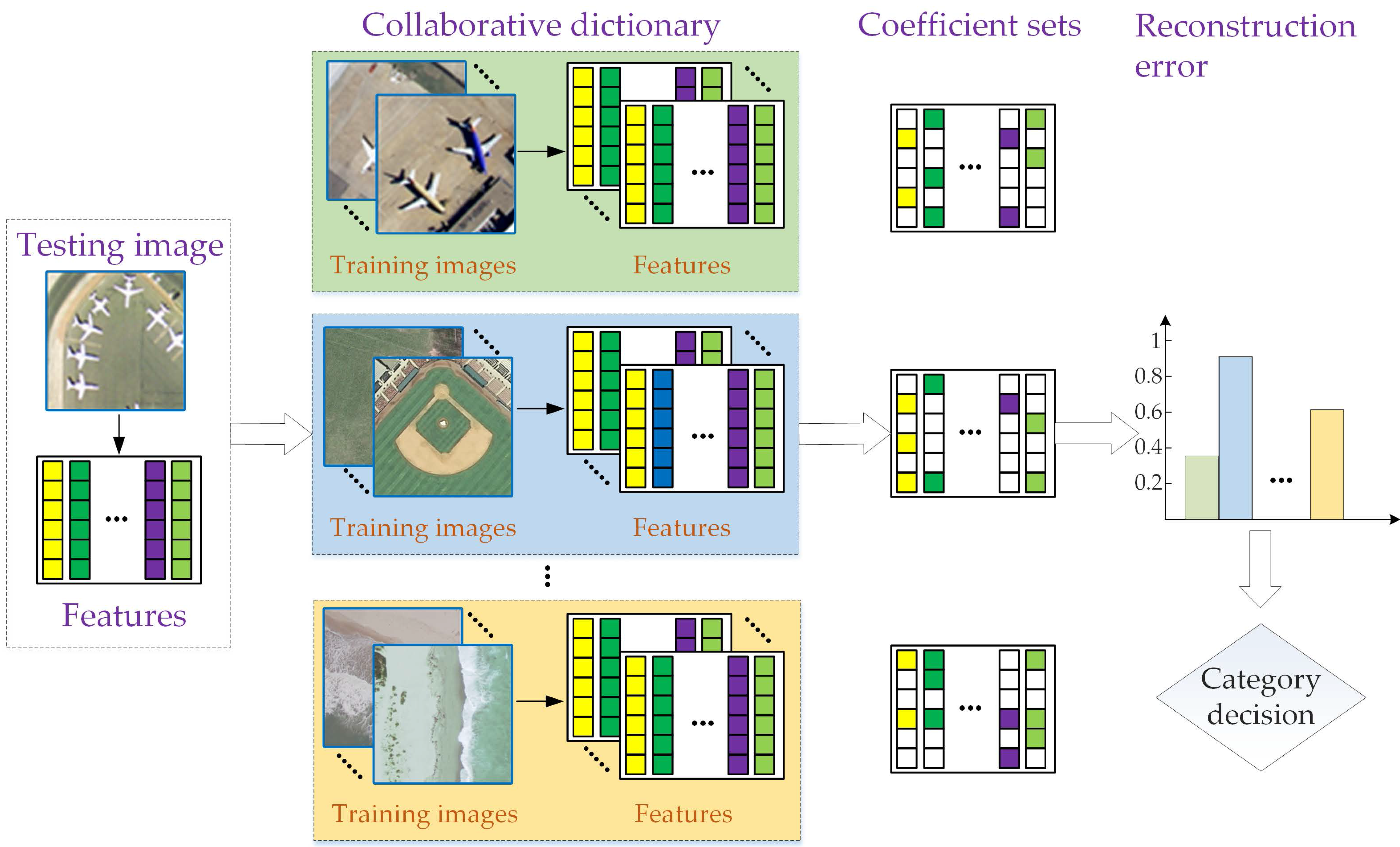
3. The Proposed Method

In this section, we describe the MTJSLRC method that makes use of sparse and low-rank learning. We also present details of the optimization method based on the APG algorithm [32,47] resorting in our method.

3.1. Sparse and Low-Rank Representation

The MTJSRC model described in the previous section considered the sparse patterns from multiple related tasks (multiple features and instances). However, in the HRS image classification, the underlying predictive classifiers lie in a hypothesis space of some low-rank structure for the redundancy and correlation in highly correlated tasks. In this paper, we consider both the sparse and low-rank patterns for multiple features and instances-based HRS image classification to improve performance. Figure 2 shows the intuition of the sparse and low-rank representation. We represent each modality of testing features as a linear combination of the corresponding training features per class by encouraging sparsity and low-rankness among features. Thus, we focus on the usage of the sparse penalty and low-rank constraint to enforce joint sparsity and low-rank structure across representation tasks.

3.2. Class-Level Joint Sparse and Low-Rank Regularization

In the MTJSRC method, the formulation of problem Equation (4) improves the independent learning model Equation (2) to a joint learning model by imposing a class-level sparsity-inducing term. It can be useful to represent a testing image by a few training samples under the common class for the multi-class classification. To encourage the low-rank structure in the model coefficient, we impose a class-level rank-constraint term to capture the underlying relationship among the tasks for improving generalization performance. Therefore, the representation of multiple features and instances may share certain class-level sparse and low-rank patterns.

To consider the low-rank structure within class $j$, we apply rank constraint over $W_j$. We employ $l_1$-norm across the rank constraint of $W_j$ to reduce the redundancy in highly correlated tasks for HRS image classification. We denote the class-level rank constraint term as follows:

$$\mathrm{\Gamma }\left(W\right)={\Vert \left[rank\left(W_1\right),\cdots ,rank\left(W_J\right)\right]\Vert }_1={{\displaystyle \sum }}_{j=1}^{J}rank\left(W_j\right),$$

(8)

We propose to solve the following multi-task joint sparse and low-rank representation model:

$$\widehat{W}=\underset{W}{\arg \min }f\left(W\right)+\mathsf{\alpha }P\left(W\right)+\mathsf{\beta }\mathrm{\Gamma }\left(W\right),$$

(9)

where the expressions of $f\left(W\right)$, $P\left(W\right)$, and $\mathrm{\Gamma }\left(W\right)$ are given in Equations (5), (6) and (8) respectively, and $\mathsf{\alpha }$ and $\mathsf{\beta }$ are the regularization coefficients to balance the strength of the general loss component and regularization terms. The problem Equation (9), however, is non-convex and the solution may not be unique due to the rank-constraint in $\mathrm{\Gamma }\left(W\right)$, which can be regarded as $l_0$-norm of its singular value matrix. To make the problem tractable, we relax the rank operator with nuclear norm, and rewrote the model as follows:

$$\widehat{W}=\underset{W}{\arg \min }f\left(W\right)+\mathsf{\alpha }P\left(W\right)+\mathsf{\beta }Q\left(W\right),$$

(10)

where $Q\left(W\right)$ is the following $l_1$-norm across the nuclear norm:

$$\mathrm{Q}\left(W\right)={\Vert \left[{\Vert W_1\Vert }_{*},\cdots ,{\Vert W_J\Vert }_{*}\right]\Vert }_1={{\displaystyle \sum }}_{j=1}^J{\Vert W_j\Vert }_{*},$$

(11)

The classification rule of our model, therefore, is identical with MTJSRC. We call the model Equation (10) together with the decision rule Equation (7) MTJSLRC, namely multi-task joint sparse and low-rank representation and classification.

3.3. Optimization Algorithm

The objective function Equation (10) consists of a squared reconstruction error term $f\left(W\right)$, a non-smooth $l_{1,2}$-norm regularization term $P\left(W\right)$, and a non-smooth $l_1$-norm across low-rank regularization term $Q\left(W\right)$. The problem is intractable for the two non-smooth convex regularization terms $P\left(W\right)$ and $Q\left(W\right)$. Considering a general minimization problem of the objective composing a smooth convex term and a non-smooth convex term, Nesterov et al. [47] proposed the APG method achieving $\mathrm{O}\left(1/t^2\right)$ rate of convergence. Chen et al. [49] applied a nearly unified treatment using existing APG methods to group/multi-task joint sparse learning. Similar to [49], Yuan et al. implemented an APG optimization procedure for MTJSRC [32]. In this paper, we solve the problem (10) by transforming it to a combination of a smooth convex term and a non-smooth term. Then, we can apply the APG algorithm as used in MTJSRC to optimize our objective function.

We adopt the Moreau Proximal Smoothing [50] on the nuclear norm regularization term in $Q\left(W\right)$. More formally, the nuclear norm $\mathsf{\beta }{\Vert W_m\Vert }_{*}$ is approximated by Moreau approximation

$${\mathrm{\Phi }}_{\mathsf{\mu }}\left(W_j\right)=\underset{G}{\min }(\frac{1}{2\mathsf{\mu }}{\Vert W_j-G\Vert }_F^2+\mathsf{\beta }{\Vert W_j\Vert }_{*}),$$

(12)

where $\mathsf{\mu }$ is the smoothing parameter. The ${\mathrm{\Phi }}_{\mathsf{\mu }}\left(W_j\right)$ is convex and smooth with respect to $W_j$, and the gradient can be computed as

$$\nabla {\mathrm{\Phi }}_{\mathsf{\mu }}\left(W_j\right)=\mathsf{\beta }\left(W_j-G^{*}\left(W_j\right)\right),$$

(13)

where $G^{*}\left(W_j\right)=\arg \underset{G}{\min }(\frac{1}{2\mathsf{\mu }}{\Vert W_j-G\Vert }_F^2+\mathsf{\beta }{\Vert G\Vert }_{*})$ The closed-form expression of $G^{*}\left(W_j\right)$ can be determined using the soft-threshold operation on the singular values of $W_j$ [46], and the gradient can be denoted as

$$\nabla \mathrm{\Phi }\left(W_j\right)=\mathsf{\beta }\left(W_j-U{\mathrm{\Sigma }}_{\mathrm{\lambda }}{\mathrm{V}}^{\mathrm{T}}\right),$$

(14)

where $W_j=U{\mathrm{\Sigma }\mathrm{V}}^{\mathrm{T}}$ is the singular value decomposition of $W_j$, ${\mathrm{\Sigma }}_{\mathrm{\lambda }}$ is diagonal with ${\left({\mathrm{\Sigma }}_{\mathrm{\lambda }}\right)}_{ii}=\max \left(0,{\mathrm{\Sigma }}_{ii}-\mathrm{\lambda }\right)$, and $\mathrm{\lambda }=\mathsf{\beta }/\mathsf{\mu }$. Therefore, we apply the following smoothing function to the class-level rank constraint term $Q\left(W\right)$, and the approximation is:

$$\mathrm{\Omega }\left(W\right)={{\displaystyle \sum }}_{j=1}^J{\mathrm{\Phi }}_{\mathsf{\mu }}\left(W_j\right),$$

(15)

The $\mathrm{\Omega }\left(W\right)$ is convex and smooth due to ${\mathrm{\Phi }}_{\mathsf{\mu }}\left(W_j\right)$ is convex and smooth, and the gradient is:

$$\nabla \mathrm{\Omega }\left(W\right)={{\displaystyle \sum }}_{j=1}^J{\mathrm{\Phi }}_{\mathsf{\mu }}\left(W_j\right),$$

(16)

We replace the nuclear norm with its Moreau approximation in model Equation (12) and obtain the approximated objective with only one non-smooth term.

$$\widehat{W}=\underset{W}{\arg \min }f\left(W\right)+\mathsf{\alpha }P\left(W\right)+\mathsf{\beta }\mathrm{\Omega }\left(W\right),$$

(17)

We define the smooth component in Equation (17) as $H\left(W\right)=f\left(W\right)+\mathsf{\beta }\mathrm{\Omega }\left(W\right)$. The objective function can be seen as the summation of a smooth term $H\left(W\right)$ and a non-smooth $l_{1,2}$-norm regularization term $\mathsf{\alpha }P\left(W\right)$.

$$\widehat{W}=\underset{W}{\arg \min }H\left(W\right)+\mathsf{\alpha }P\left(W\right),$$

(18)

Then, we can use the APG optimization algorithm to solve problem Equation (18).

Algorithm 1 summarizes the details of optimization and classification. As MTJSRC in [32], each iteration consists of the generalized gradient mapping step and the aggregation forward step. The difference between MTJSRC and MTJSLRC is the gradient calculation in generalized gradient mapping step. We update the $W^{\left(t+1\right)}$ using current matrix $V^{\left(t+1\right)}$ in the generalized gradient mapping step as follows:

$$W^{\left(t+1\right)}=\underset{W}{\arg \min }H(V^{\left(t\right)})+\langle \nabla H(V^{\left(t\right)}),(W-V^{\left(t\right)})\rangle +\frac{1}{2\mathrm{\lambda }}{\Vert W-V^{\left(t\right)}\Vert }_F^2+\mathsf{\alpha }{\Vert W\Vert }_{1,2},$$

(19)

where $\mathrm{\lambda }$ is the step-size parameter. The solution of problem shown in [51] is:

$$U^{\left(t\right)}=V^{\left(t\right)}-\mathrm{\lambda }\nabla H\left(V^{\left(t\right)}\right),$$

(20)

$$W_j^{\left(t+1\right)}=\max (0,\left[1-\frac{\mathsf{\alpha }\mathrm{\lambda }}{\Vert U_j^{\left(t\right)}\Vert }\right])·U_j^{\left(t\right)},$$

(21)

Then, we apply the aggregation forward step to update $V^{\left(t\right)}$ as follows:

$$V^{\left(t+1\right)}=W^{\left(t+1\right)}+\frac{{\mathsf{\theta }}_t-1}{{\mathsf{\theta }}_{t+1}}(W^{\left(t+1\right)}-W^{\left(t\right)}),$$

(22)

$${\mathsf{\theta }}_{t+1}=\frac{1}{2}(1+\sqrt{1+4{\mathsf{\theta }}_t^2})$$

(23)

Since the convergence is not necessary for the good classification performance, we take the account of the maximum number of iterations which is denoted as $T$ in Algorithm 1.

Algorithm 1: MTJSLRC Algorithm

Inputs:   The training image feature matrices, $\{X^k,k=1,\dots ,K\}$;   All testing image features, $\{y^{kl},k=1,2,\cdots ,K,l=1,2,\cdots ,L\}$;   The regularization parameters, $\mathsf{\alpha }>0$, $\mathsf{\beta }>0$;   The step-size parameter, $\mathrm{\lambda }>0$;   The maximum number of iteration, $T$; Output:   The representation coefficients, $W^{\left(t\right)}$;   The predicted labels for testing image scenes, $\widehat{j}$; Initialization:   $W_0=V_0=0$, ${\mathsf{\theta }}_0=1$, $t=0$  1: repeat:  2:  Calculate $U^{\left(t\right)}=V^{\left(t\right)}-\mathrm{\lambda }\nabla H\left(V^{\left(t\right)}\right)$, in which $\nabla H\left(V^{\left(t\right)}\right)$ is given by $$\nabla H\left(V^t\right)=\nabla f\left(V^{\left(t\right)}\right)+\mathsf{\beta }\nabla \mathrm{\Omega }\left(V^{\left(t\right)}\right),$$ (24) $${[\nabla f\left(V^{\left(t\right)}\right)]}^{kl}=-{(X^k)}^T{y}^{kl}+{(X^k)}^T{X}^k{\left[V^{\left(t\right)}\right]}^{kl},$$ (25) $${[\nabla \mathrm{\Omega }\left(V_j^{\left(t\right)}\right)]}^{kl}={(\nabla {\mathrm{\Phi }}_{\mathsf{\mu }}\left(V_j^{\left(t\right)}\right))}^{kl},$$ (26)     $l=1,\dots ,\mathrm{L},k=1,\dots ,K,j=1,\dots ,J$  3:  Calculate $W_j^{\left(t+1\right)}$ as     $W_j^{\left(t+1\right)}=\max (0,\left[1-\frac{\mathsf{\alpha }\eta }{\Vert U_j^{\left(t\right)}\Vert }\right])·U_j^{\left(t\right)}$, $j=1,\dots ,J$  4:  Set ${\mathsf{\theta }}_{t+1}=\frac{1}{2}(1+\sqrt{1+4{\mathsf{\theta }}_t^2})$  5:  Update $V^{\left(t+1\right)}=W^{\left(t+1\right)}+\frac{{\mathsf{\theta }}_t-1}{{\mathsf{\theta }}_{t+1}}\left(W^{\left(t+1\right)}-W^{\left(t\right)}\right)$  6:  Set $\mathrm{t}\leftarrow \mathrm{t}+1$  7: until converges or $\mathrm{t}>\mathrm{T}$; 8: Calculate $\widehat{j}=\mathit{arg}\mathit{min}{{\displaystyle \sum }}_{k=1}^K{{\displaystyle \sum }}_{l=1}^L{\Vert y^{kl}-X_j^k{W}_j^{kl}\Vert }^2$

3.4. Time Complexity Analysis

Due to the iterative characteristic of MTJSLRC, the computational complexity depends on two factors, the number of iterations before convergence and the time consumed at each iteration. As MTJSRC, the objective of our proposed model also is to minimize the reconstruction error of a testing image; therefore, it is not necessary to execute the algorithm until convergent for the best recognition performance. Therefore, we consider the dominant computational cost at each iteration of Algorithm 1, which comes from the calculation of Equations (25) and (26) in step 2. As the gradient estimation in [34], the first term $-{(X^k)}^T{y}^{kl}$ in Equation (25) can be pre-computed. Assume $\mathrm{T}$ be the average number of iterations for the running of Algorithm 1, then the total Floating-point operations (Flops) for gradient estimation of Equation (25) in step 2 is $O\left(KLn{d}_k+2TKLn{d}_k\right)$ as estimated in [32]. The time-consuming part of Equation (26) are SVD of matrix $V_j^{\left(t\right)}$ and the $U{\mathrm{\Sigma }}_{\mathrm{\lambda }}{\mathrm{V}}^{\mathrm{T}}$ in $\nabla {\mathrm{\Phi }}_{\mathsf{\mu }}$($V_j^{\left(t\right)}$). The costs of the two terms are typically $\mathrm{O}\left(s\right)$ and $\mathrm{O}(2{\left(KL\right)}^2{n}_j)$ Flops, respectively, where $s$ is the average computation time for the SVD of $V_j^{\left(t\right)}$. The total Flops consumed by gradient estimation in Equation (24) are typically $\mathrm{O}(KLn{d}_k+T(2KLn{d}_k+Js+2J{\left(KL\right)}^2{n}_j))$. The time consumed in the other steps is negligible in comparison to that of gradient estimation in step 2.

4. Experiments and Analysis

In this section, we provide the experimental setup, and discuss the results on two public datasets. We conducted several groups of experiments to evaluate the capability and effectiveness of MTJSLRC for HRS image classification.

4.1. Experimental Setup

We evaluated our proposed MTJSLRC method on two public land-use scene datasets, which were:

• UC Merced Land Use Dataset. The UC Merced dataset (UCM) [10] is one of the first ground truth datasets derived from a publicly available high resolution overhead image; it was manually extracted from aerial orthoimagery and downloaded from the United States Geological Survey (USGS) National Map. This dataset contains 21 typical land-use scene categories, each of which consists of 100 images measuring $256\times 256$ pixels with a pixel resolution of 30 cm in the red-green-blue color space. Figure 3 shows two examples of ground truth images from each class in this dataset. The classification of UCM dataset is challenging because of the high inter-class similarity among categories such as medium residential and dense residential areas.
• WHU-RS Dataset. The WHU-RS dataset [52] is a new publicly available dataset wherein all the images are collected from Google Earth (Google Inc. Mountain View, CA, USA). This dataset consists of 950 images with a size of $600\times 600$ pixels distributed among 19 scene classes. Examples of ground truth images are shown in Figure 4. It can be seen that, as compared to the UCM dataset, the scene categories in the WHU-RS dataset are more complicated due to variations in scale, resolution, and viewpoint-dependent appearance.

For the testing image, we utilize four types of transform to obtain multiple instances as follows: zoom it in 1.2, flip it left to right, and rotate it five degrees clockwise and counterclockwise. Therefore we utilized $L=4$ instances for each testing image in the MTJSRC and MTJSLRC models. We give an overview of the features used in our experiments, and refer to the corresponding publications for more details:

• Bag of Visual Words (BoVW). We extracted Scale-Invariant Feature Transform (SIFT) descriptors [18] using a dense regular grid on the image with image patches at a $16\times 16$ pixel size over a grid with spacing of eight pixels [22]. The visual vocabulary containing 600 entries was formed by k-means clustering of a random subset of patches from the training set.
• Multi-Segmentation-based correlaton (MS-based correlaton) [8]. SIFT descriptors were extracted on a regular grid with a spacing of eight pixels and at $16\times 16$ pixel grid size. The segmentation size was set at six and the number of segments were $\left\{2^2,2^3,2^4,2^5,2^6,2^7\right\}$. The MS-based correlograms were quantized in 300 MS-based correlatons using k-means.
• Dense words (including PhowGray, PhowColor) [11]. The PhowGray was modeled using rotationally invariant SIFT descriptors computed on a regular grid with the step of five pixels at four multiple scales (5, 7, 9, 12 pixel radii), zeroing the low contrast pixels. Then the descriptors were subsequently quantized into a vocabulary of 600 visual words that were generated by k-means clustering. The PhowColor is the color version of PhowGray that stacks SIFT descriptors for each HSV color channel.
• Self-SIMilarity features (SSIM). SSIM descriptors [12] were extracted on a regular grid at steps of five pixels. We acquired each descriptor by computing the correlation map of a $5\times 5$ pixels patch in a window of radius 40 pixels, quantizing it in 3 radial bins and 10 angular bins. This way, we obtained a pack of 30 dimensional descriptor vectors. These descriptors were then quantized into 600 visual words.

We computed all but the MS-based correlaton features in a spatial pyramid as proposed in [22]. A pyramid representation consists of several levels obtained by partitioning the image into increasingly fine non-overlapping sub-regions and computing histograms of features found inside each sub-region. The features of each level were concatenated to build the final descriptor. We computed a three-level pyramid of spatial histograms for each feature channel. In the experiment, we divided the dataset 10 times to obtain reliable results, and all the final results, as well as the classification accuracy rate for categories were recorded as the mean and standard deviation of these 10 runs.

The features were computed using open source code [53]. All experiments in this work are implemented var Matlab 8.0/Windows 10, and run on a workstation equipped with 4 Intel quadcore 3.3 GHz CPUs with 16 GB memory.

4.2. Experimental Results

4.2.1. Explanation of Feature Combination

We applied the UCM dataset to demonstrate the feature combination capability of MTJSLRC. For each image, we set $K=2$ for feature combination, including the SSIM and BoVW features. These two features are complementary in terms of co-occurrence of local patches and appearance. We used $L=4$ instances for each testing image by transformation, and obtained $K\times L=2\times 4$ representation tasks. The number of training images was varied using $N_m=\left\{10,20,30,40,50,60,70,80,90\right\}$ per category for training and the remaining images for testing.

Figure 5 shows the classification accuracy results of individual features by SRC and their combination with MTJSRC and MTJSLRC. The MTL-based models including the MTJSRC and MTJSLRC models improved the performance by feature combination. We can see that the performance improved as the training ratio increased since more data became available for model training. Moreover, the average accuracy approached 80% as the number of training images per category was 20. This indicates that the SRC and MTL can handle the “lack of samples” problem in HRS image recognition. Compared with the MTJSRC model, our MTJSLRC method improved classification accuracy slightly for a low number of tasks. The low-rank structure had no significant effect on the MTJSRC whereas the class-level coefficient $rank\left(W_m\right)$ was less than or equal to the number of tasks.

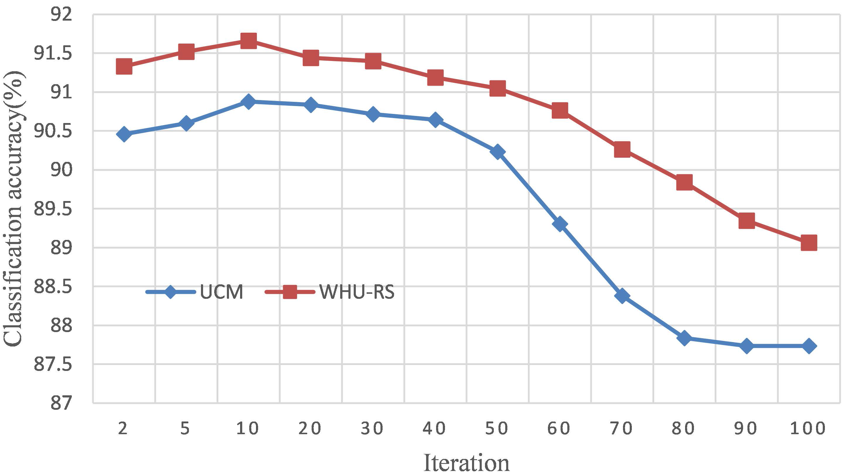
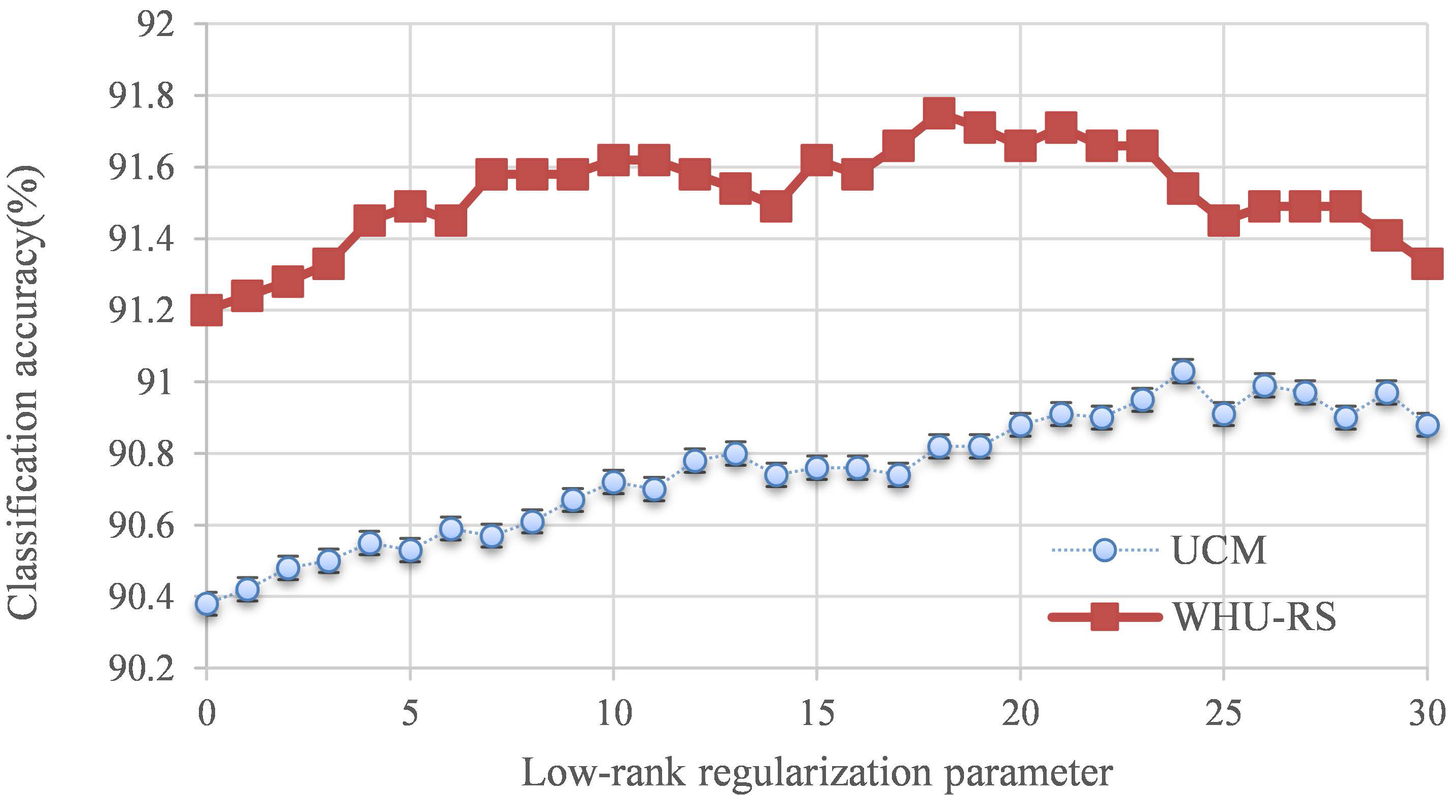
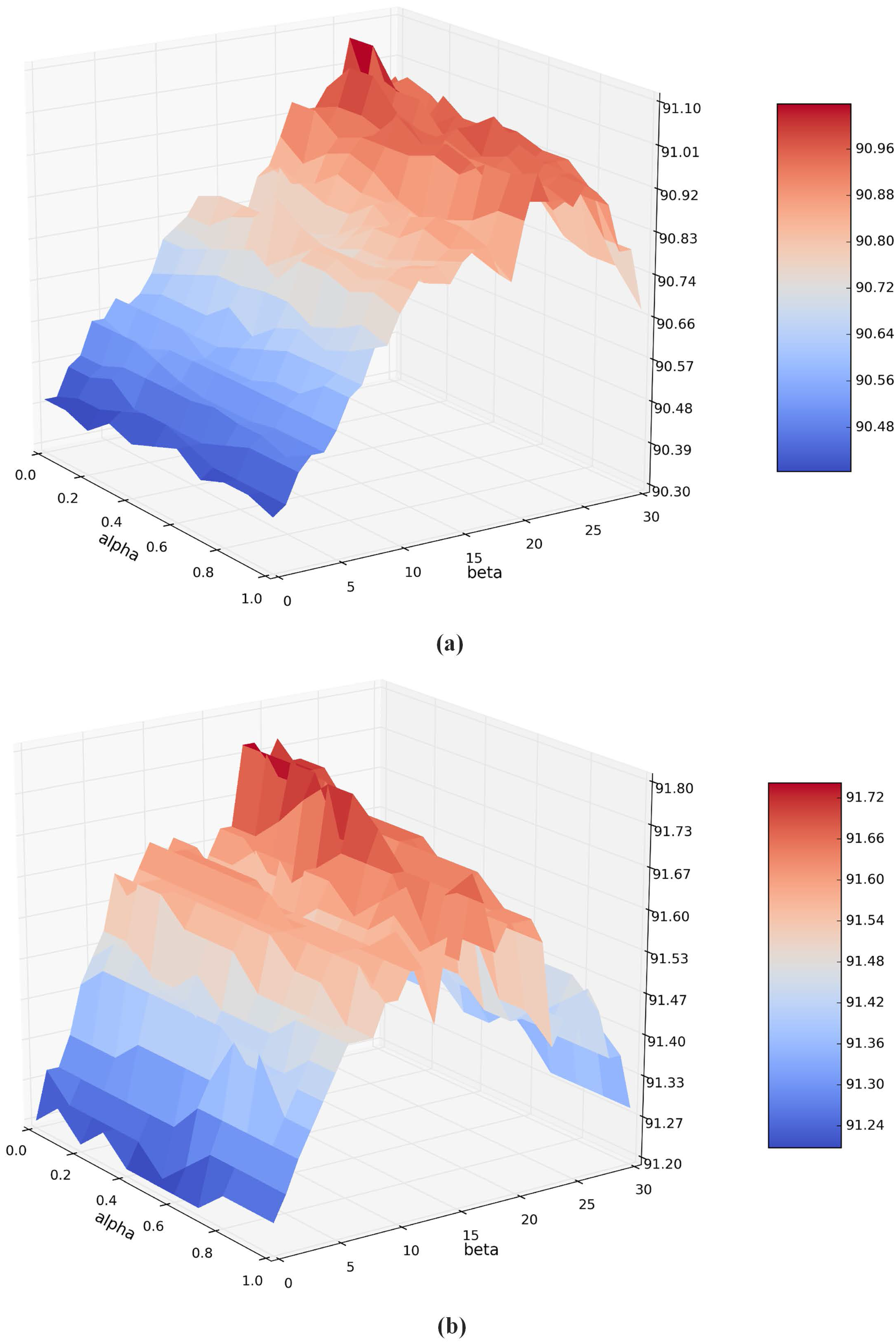
4.2.2. Parameter Effect

We investigated the effect of iteration on classification performance (Figure 6). As stated in [32], the APG algorithm has been shown to be convergent to global minimum at the optimal rate $O\left(1/t^2\right)$, but this algorithm does not guarantee a monotonic decrease in objective value. Fortunately, the convergence, which may need several hundred iterations, is not necessary for good classification performance.

The results displayed in Figure 6 show that the performance can achieve a sufficient classification performance within just a few iterations. The best performance on the two datasets consistently occurs at about 10 iterations. As proposed in [32], the MTJSRC and our proposed methods both are aimed at addressing minimal reconstruction error on a testing image, while those classifier training-based methods directly optimize the classification error on training data.

There are two other parameters that affect the classification performance, including the regularization coefficients for class-level sparsity and low-rank constraint. We analyze the effects of the parameters on the classification accuracy to choose the optimal parameters. These regularization coefficients determine the strength of the loss and regularization terms. Intuitively, there is actually a trade-off between the sparse structure and low-rank structure. Let us consider several special cases of our formulation: when $\mathsf{\alpha }=0$, the problem degenerates to a model with only a low-rank structure that learns a small number of shared features among tasks; when $\mathsf{\beta }=0$, the problem degenerates into a model with only a sparse structure term among tasks. To take advantage of both properties, we adjust $\mathsf{\alpha }$ and $\mathsf{\beta }$ to balance the sparse and low-rank structures.

We tested a series of $\mathsf{\alpha }$ and $\mathsf{\beta }$ on the UCM and WHU-RS datasets, and the classification results are shown in Figure 7. The sparse regularization parameter was selected from the range $\mathsf{\alpha }\in \left\{0,0.1,0.2,\dots ,1\right\}$, and the low-rank regularization parameter $\mathsf{\beta }\in \left\{0,1,2,\dots ,30\right\}$ was selected for these two datasets. From Figure 7, we can observe that MTJSLRC achieves the best results at most of settings for these two datasets. This verifies the capability and benefits of MTJSLRC when simultaneously learning low-rank and sparse structures from multiple tasks. For the low-rank regularization coefficient, the classification accuracy on the UCM and WHU-RS datasets takes on an overall trend that first improves, then comes to its maximum, and begins to gradually decrease. The optimal low-rank regularization coefficient was around 25 to the UCM dataset and 20 to the WHU-RS dataset for most of the sparse regularization parameter. This demonstrates the significance of the low-rank structure for these multiple feature combination tasks based on MTL and SRC. The variation of performance to the sparse regularization parameter $\mathsf{\alpha }$ was relatively smooth in comparison to the low-rank regularization coefficient. The overall optimal $\mathsf{\alpha }$ was both around 0.1 for these two datasets.

To better visualize this phenomena, we selected $\mathsf{\alpha }=0.1$ to distinguish effects of the low-rank regularization parameter $\mathsf{\beta }$ on these two datasets. As shown in Figure 8, the trend in the classification accuracy is not easy to see. This is probably because the convergence of our objective function to minimizer is no guaranteed, and the objective value does not monotonically decrease. On the whole, however, the performance first improves and then gradually drops with the increase of $\mathsf{\beta }$, and the best performance occurs at $\mathsf{\beta }=24$ for the UCM dataset and $\mathsf{\beta }=18$ for the WHU-RS dataset. The results show clearly that the multiple tasks in MTJSLRC share one low-dimension feature space assumed as low-rank structure in this paper. The low-rank regularization parameter $\mathsf{\beta }$ indeed had a substantial impact on final performance, and overlooking the low-rank structure for these two datasets would have negatively compromised the results.

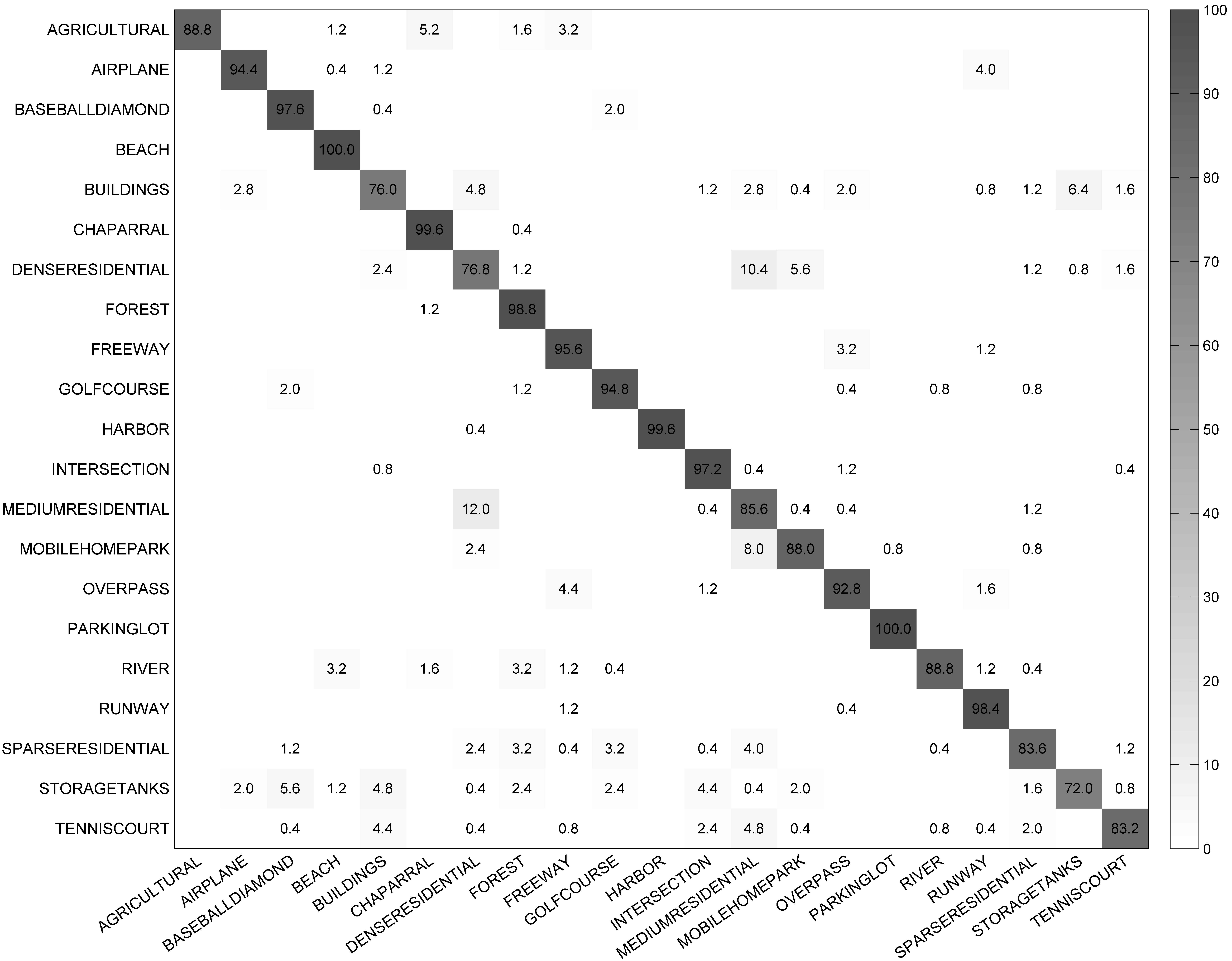
4.2.3. Classification Results

We applied the MTJSLRC to HRS image classification on the UCM and WHU-RS datasets. In addition, to further illustrate the effect of our method, we compared our MTJSLRC method with the following methods:

• Feature combination based on independent SRC. This method can be seen as a simplification of the MTJSLRC method without the joint sparsity and low-rank structure across tasks. Thus, the coefficients $\widehat{W}$ are independently learned by SRC.
• Feature combination based on MTJSRC. This method enforces the joint sparsity across tasks but ignore the low-rank structure in the multiple feature space.
• The representative multiple kernel learning method. The kernel matrices are computed as $\exp \left(-{\chi }^2\left(\mathrm{x},x^{\prime }\right)/\mathsf{\mu }\right)$, where $\mathsf{\mu }$ is set to be the mean value of the pairwise ${\chi }^2$ distance on the training set.

The classification accuracy of our MTJSLRC along with baselines and results from several representation methods on the UCM dataset are shown in

Table 1. Accuracy (mean ± std %) performance on the UCM dataset.

(a) Single Features
Features	SVM	SRC
BoVW	80.21 $\pm$ 1.6	79.92 $\pm$ 0.83
PhowColor	87.46 $\pm$ 1.7	86.99 $\pm$ 0.85
PhowGray	85.87 $\pm$ 1.75	86.35 $\pm$ 0.59
SSIM	80.95 $\pm$ 1.26	80.38 $\pm$ 1.27
MS-based Correlaton	81.73 $\pm$ 1.15	81.12 $\pm$ 0.86
(b) Feature Combination Methods
Methods	Accuracy
SRC	90.03 $\pm$ 0.78
MKL	90.15 $\pm$ 0.96
MTJSRC	90.45 $\pm$ 0.53
MTJSLRC	91.07 $\pm$ 0.67

. The results on single feature are listed in Table 1(a). We can observe that SRC-based methods yield comparable accuracies to SVM on single features. The results by feature combination methods are tabulated in Table 1(b). It can be seen that all feature combination methods dramatically improve classification performance, but our MTJSLRC-based algorithm is slightly better than the SRC-based combination method, the MTJSRC-based method, and the MKL method. The independent SRC combination, a simplification of MTJSRC or the MTJSLRC-based method, competes with the MKL. By considering the joint sparsity across different tasks, the MTJSRC-based algorithm is superior to the independent SRC combination methods, even better than the MKL, but slightly inferior to our MTJSLRC method that takes into account the low-rank structure from multiple tasks. Like the SRC-based combination and MTJSRC-based methods, our MTJSLRC method does not require any classifier training procedures. Thus it is flexible in practice, and novel reference samples can be introduced without additional efforts to update the classifier.

The HRS image classification results on the WHU-RS dataset are listed in

Table 2. Accuracy (mean ± std %) performance on the WHU-RS dataset.

(a) Single Features
Features	SVM	SRC
BoVW	85.68 $\pm$ 1.07	85.85 $\pm$ 0.95
PhowColor	86.84 $\pm$ 1.39	88.04 $\pm$ 1.32
PhowGray	85.05 $\pm$ 1.48	84.04 $\pm$ 0.96
SSIM	84.9 $\pm$ 2.18	82.32 $\pm$ 1.02
MS-based Correlaton	87.72 $\pm$ 1.42	87.12 $\pm$ 1.7
(b) Feature Combination Methods
Methods	Accuracy
SRC	91.2 $\pm$ 1.03
MKL	91.67 $\pm$ 0.95
MTJSRC	91.45 $\pm$ 0.98
MTJSLRC	91.74 $\pm$ 1.14

. Table 2(a) lists the results on a single feature, which indicate that SRC methods are competitive to SVM for single features on this dataset. Table 2(b) shows the results from feature combination methods. We can see that our algorithm performs comparably to the MKL method, and superior to the independent SRC combination and MTJSRC methods.

The classification performances of individual classes on the UCM and WHU-RS datasets using our proposed MTJSLRC method with the optimal parameters as previously described are shown in the confusion matrices shown in Figure 9. As observed, there is some confusion between certain scenes in the UCM dataset. The identified positive samples for the storage tanks display the greatest confusion because their color information, spatial information, and texture information are likely to be confused with those of baseball diamond, buildings, intersections, forests, golf courses, airplane fields, and mobile home parks. The most confusing pairs were median residential and dense residential with the misclassification rate reaching 12% because of the strong similarity of these scenes. Therefore, the features used in our research were not sufficient for separating these scenes, and additional features must be included in our future work.

The classification results on the WHU-RS dataset are illustrated in Figure 10. Based on the fusion of the visual effect, deserts, football fields, parks, ponds, mountains, and viaducts achieve the best results at over 97%; residential areas are mixed with commercial, and industrial areas are mixed with residential. This may result from the strong similarity of these scenes and intuitively, give rise to weak performance.

4.2.4. Running Time

In this experiment, we analyzed the running times for different models on the UCM and WHU-RS datasets. As shown in

Table 3. Running time comparison (total/per-image in seconds).

Methods	UCM		WHU-RS
	Training	Testing	Training	Testing
SRC	0	94.27/0.09	0	45.42/0.096
MKL	992.18/0.945	1.07/0.001	345.24/0.727	0.64/0.001
MTJSRC	0	124.98/0.119	0	58.17/0.122
MTJSLRC	0	389.2/0.37	0	179.57/0.378

, the per query times of our method were 0.37 s for the UCM dataset and 0.378 s for the WHU-RS dataset, while per query times were 0.09 s and 0.096 s for the SRC combination method, and 0.119 s and 0.122 s for the MTJSRC method. The running time of the MKL method was much longer than the others on account of the required training phase.

5. Discussion

HRS image classification plays an important role in understanding remotely sensed image. In our work, we built a multi-task joint sparse and low-rank representation for HRS image classification. Our objective is to improve the classification accuracy by fusing multiple features and instances. Experimental results on the UCM and WHU-RS datasets indicate that the proposed MTJSLRC model is competitive with other feature combination methods for HRS image classification.

From the experiments on feature combination illustrated in Figure 4, we observe that the multi-task joint sparse representations method is a simple yet effective way to fuse multiple complementary visual features and instances to improve the accuracy. By considering the low-rank structure, our MTJSLRC model achieved slightly more accurate results than the MTJSRC model for multiple tasks. The performance was competitive even when the number of samples for learning was small. This benefits from MTL as it transfers knowledge from one task to another.

We tested three important parameters of the MTJSLRC method in experiments. As shown in Figure 6, we found that the convergence is not necessary and the algorithm can achieve good classification performance with a few iterations. This means that our proposed method requires less time overall and hence is very competitive. We see from Figure 7 and Figure 8 that the two regularization parameters for the sparse structure and low-rank structure impact the final performance. It shows improvement at first and then a gradual dropping performance trend with an increasing low-rank regularization parameter. The variation of performance along with the joint sparse regularization parameter is relatively stable for two datasets as discussed in this paper. Our experiments show that the low-rank regularization parameter ranging from 20 to 25 is suitable for the best accuracy. The joint sparse regularization parameter as 0.1 is sufficient to result in good performance. Table 1 and Table 2 show that our method can fuse multiple complementary visual features and instances to improve classification accuracy. The proposed MTJSLRC method achieves better classification results than the MTJSRC method, which ignores the low-rank structure across tasks, and is slightly superior to MKL.

The proposed MTJSLRC method performs quite competitively with several representative approaches by fusing multiple complementary features and instances, thus considering the sparse and low-rank structure across tasks. However, our MTJSLRC method is inferior in terms of computational speed when compared to other representative methods since the SVD algorithm is used in the optimal solution. By considering the computational complexity, we only use four transformed instances for each testing image. In future work, we plan to improve MTJSLRC by elaborating on optimal schemes with increased instances to add more robustness and cope with variations in scales, translation and rotation, thereby making it more efficient.

6. Conclusions

This paper presents the Multi-Task Joint Sparse Representation Classification (MTJSLRC) algorithm for High-Resolution Satellite (HRS) image scenes classification. In the Multi-Task Learning (MTL) framework, both sparse and low-rank structures are important but quite different in nature. We argue that the multi-task joint sparse and low-rank representation is a simple yet effective way to fuse multiple complementary features and instances. Compared to the MTJSRC method that only considers sparse structure, our proposed method can improve classification performance by learning low-rank and sparse structures simultaneously. Experiments on the UC Merced (UCM) and WHU-RS datasets indicate that our method performs quite competitively with several representative approaches. Similar to the SRC and MTJSRC methods, our proposed method is free of classifier training, which is convenient to introduce novel reference samples and classifier updates. On the whole, multi-task joint sparse and low-rank representation is a promising method for scene classification with multiple features and/or instances in terms of accuracy and computational cost. In future work, we will incorporate additional texture, shape, or structural features that are more appropriate for HRS image scene classification, especially integrating various deep convolutional neural networks for better representation. In addition, another practical research direction would be to accelerate the speed of the algorithm.

References

1. Prasad, S.; Bruce, L.M. Decision fusion with confidence-based weight assignment for hyperspectral target recognition. IEEE Trans. Geosci. Remote Sens. 2008, 46, 1448–1456. [Google Scholar] [CrossRef]
2. Bruzzone, L.; Carlin, L. A multilevel context-based system for classification of very high spatial resolution images. IEEE Trans. Geosci. Remote Sens. 2006, 44, 2587–2600. [Google Scholar] [CrossRef]
3. Rizvi, I.A.; Mohan, B.K. Object-based image analysis of high-resolution satellite images using modified cloud basis function neural net-work and probabilistic relaxation labeling process. IEEE Trans. Geosci. Remote Sens. 2011, 49, 4815–4820. [Google Scholar] [CrossRef]
4. Bellens, R.; Gautama, S.; Martinezfonte, L.; Philips, W.; Chan, J.C.; Canters, F. Improved classification of VHR images of urban areas using directional morphological profiles. IEEE Trans. Geosci. Remote Sens. 2008, 46, 2803–2813. [Google Scholar] [CrossRef]
5. Blaschke, T. Object based image analysis for remote sensing. ISPRS J. Photogramm. Remote Sens. 2010, 65, 2–16. [Google Scholar] [CrossRef]
6. Yu, H.; Yang, W.; Xia, G.; Liu, G. A color-texture-structure descriptor for high-resolution satellite image classification. Remote Sens. 2016, 8, 30259–30292. [Google Scholar] [CrossRef]
7. Hu, F.; Xia, G.S.; Hu, J.; Zhang, L. Transferring deep convolutional neural networks for the scene classification of high-resolution remote sensing imagery. Remote Sens. 2015, 7, 14680–14707. [Google Scholar] [CrossRef]
8. Qi, K.; Wu, H.; Shen, C.; Gong, J. Land-use scene classification in high-resolution remote sensing images using improved correlatons. IEEE Geosci. Remote Sens. Lett. 2015, 12, 2403–2407. [Google Scholar]
9. Xia, G.S.; Wang, Z.; Xiong, C.; Zhang, L. Accurate annotation of remote sensing images via active spectral clustering with little expert knowledge. Remote Sens. 2015, 7, 15014–15045. [Google Scholar] [CrossRef]
10. Yang, Y.; Newsam, S. Bag-of-visual-words and spatial extensions for land-use classification. In Proceedings of the 18th SIGSPATIAL International Conference on Advances in Geographic Information Systems, San Jose, CA, USA, 3–5 November 2010; pp. 270–279.
11. Bosch, A.; Zisserman, A.; Muñoz, X. Scene classification via PLSA. In Proceedings of the 9th European Conference on Computer Vision (ECCV), Graz, Austria, 7–13 May 2006; pp. 517–530.
12. Shechtman, E.; Irani, M. Matching Local Self-Similarities across Images and Videos. In Proceedings of the IEEE Conference on Computer Vision and Pattern Recognition (CVPR), Minneapolis, MN, USA, 19–21 June 2007; pp. 1–8.
13. Bosch, A.; Munoz, X.; Marti, R. Which is the best way to organize/classify images by content? Image Vis. Comput. 2007, 25, 778–791. [Google Scholar] [CrossRef]
14. Liénou, M.; Maître, H.; Datcu, M. Semantic annotation of satellite images using latent Dirichlet allocation. IEEE Geosci. Remote Sens. Lett. 2010, 7, 28–32. [Google Scholar] [CrossRef]
15. Sheng, G.; Yang, W.; Xu, T.; Sun, H. High-resolution satellite scene classification using a sparse coding based multiple feature combination. Int. J. Remote Sens. 2012, 33, 2395–2412. [Google Scholar] [CrossRef]
16. Dai, D.; Yang, W. Satellite image classification via two-layer sparse coding with biased image representation. IEEE Geosci. Remote Sens. Lett. 2011, 8, 173–176. [Google Scholar] [CrossRef]
17. Hu, F.; Xia, G.; Hu, J.; Zhong, Y.; Xu, K. Fast Binary Coding for the Scene Classification of High-Resolution Remote Sensing Imagery. Remote Sens. 2016, 8, 70555–70578. [Google Scholar] [CrossRef]
18. Lowe, D.G. Distinctive Image Features from Scale-Invariant Keypoints. Int. J. Comput. Vis. 2004, 60, 91–110. [Google Scholar] [CrossRef]
19. Van DeWeijer, J.; Schmid, C. Coloring local feature extraction. In Proceedings of the 9th European Conference on Computer Vision (ECCV), Graz, Austria, 7–13 May 2006; pp. 334–348.
20. Ojala, T.; Pietikainen, M.; Maenpaa, T. Multiresolution gray-scale and rotation invariant texture classification with local binary patterns. IEEE Trans. Pattern Anal. Mach. Intell. 2002, 24, 971–987. [Google Scholar] [CrossRef]
21. Zhao, L.; Tang, P.; Huo, L. A 2-D wavelet decomposition-based bag-of-visual-words model for land-use scene classification. Int. J. Remote Sens. 2014, 35, 2296–2310. [Google Scholar]
22. Lazebnik, S.; Schmid, C.; Ponce, J. Beyond bags of features: Spatial pyramid matching for recognizing natural scene categories. In Proceedings of the 2006 IEEE Computer Society Conference on Computer Vision and Pattern Recognition (CVPR), New York, NY, USA, 17–22 June 2006; pp. 2169–2178.
23. Qi, K.; Zhang, X.; Wu, B.; Wu, H. Sparse coding-based correlaton model for land-use scene classification in high-resolution remote-sensing images. J. Appl. Remote Sens. 2016, 10, 042005. [Google Scholar]
24. Van De Sande, K.E.; Gevers, T.; Snoek, C.G. Evaluating color descriptors for object and scene recognition. IEEE Trans. Pattern Anal. 2010, 32, 1582–1596. [Google Scholar] [CrossRef] [PubMed]
25. Gehler, P.; Nowozin, S. On feature combination for multiclass object classification. In Proceedings of the IEEE 12th International Conference on Computer Vision, Kyoto, Japan, 29 September–2 October 2009; pp. 221–228.
26. Fernando, B.; Fromont, E.; Muselet, D.; Sebban, M. Discriminative feature fusion for image classification. In Proceedings of the IEEE Conference on Computer Vision and Pattern Recognition (CVPR), Providence, RI, USA, 16–21 June 2012; pp. 3434–3441.
27. Van de Weijer, J.; Khan, F.S. Fusing color and shape for bag-of-words based object recognition. In Proceedings of the 2013 Computational Color Imaging Workshop, Chiba, Japan, 3–5 March 2013; pp. 25–34.
28. Varma, M.; Ray, D. Learning the Discriminative Power-Invariance Trade-Off. In Proceedings of the 11th International Conference on Computer Vision (ICCV), Rio de Janeiro, Brazil, 14–20 October 2007.
29. Lin, Y.; Liu, T.; Fuh, C. Local ensemble kernel learning for object category recognition. In Proceedings of the IEEE Conference on Computer Vision and Pattern Recognition (CVPR), Minneapolis, MN, USA, 19–21 June 2007.
30. Luo, W.; Yang, J.; Xu, W.; Li, J.; Zhang, J. Higher-level feature combination via multiple kernel learning for image classification. Neurocomputing 2015, 167, 209–217. [Google Scholar] [CrossRef]
31. Vedaldi, A.; Gulshan, V.; Varma, M.; Zisserman, A. Multiple kernels for object detection. In Proceedings of the 10th International Conference on Computer Vision (ICCV), Kyoto, Japan, 27 September–4 October 2009.
32. Yuan, X.; Liu, X.; Yan, S. Visual Classification with Multitask Joint Sparse Representation. IEEE Trans. Image Process. 2012, 21, 4349–4360. [Google Scholar] [CrossRef] [PubMed]
33. Caruana, R. Multi-task learning. Mach. Learn. 1997, 28, 41–75. [Google Scholar] [CrossRef]
34. Evgeniou, T.; Pontil, M. Regularized multi-task learning. In Proceedings of the Knowledge Discovery and Data Mining, Sydney, Australia, 26–28 May 2004; pp. 109–117.
35. Wright, J.; Yang, A.Y.; Ganesh, A.; Sastry, S.S.; Ma, Y. Robust face recognition via sparse representation. IEEE Trans. Pattern Anal. Mach. Intell. 2009, 31, 210–227. [Google Scholar] [CrossRef] [PubMed]
36. Li, J.; Zhang, H.; Zhang, L.; Huang, X.; Zhang, L. Joint collaborative representation with multitask learning for hyperspectral image classification. IEEE Trans. Geosci. Remote Sens. 2014, 52, 5923–5936. [Google Scholar] [CrossRef]
37. Zhang, H.; Li, J.; Huang, Y.; Zhang, L. A nonlocal weighted joint sparse representation classification method for hyperspectral imagery. IEEE J. Sel. Top. Appl. Earth Observ. Remote Sens. 2014, 7, 2056–2065. [Google Scholar] [CrossRef]
38. Argyriou, A.; Evgeniou, T.; Pontil, M. Convex multi-task feature learning. Mach. Learn. 2008, 73, 243–272. [Google Scholar] [CrossRef]
39. Zhang, L.; Yang, M.; Feng, X.; Ma, Y.; Zhang, D. Collaborative representation based classification for face recognition. arXiv, 2012; arXiv:1204.2358. [Google Scholar]
40. Obozinski, G.; Taskar, B.; Jordan, M. Joint covariate selection and joint subspace selection for multiple classification problems. J. Stat. Comput. 2009, 20, 231–252. [Google Scholar] [CrossRef]
41. Yuan, M.; Lin, Y. Model selection and estimation in regression with grouped variables. J. R. Stat. Soc. Ser. B 2006, 68, 49–67. [Google Scholar] [CrossRef]
42. Liu, H.; Palatucci, M.; Zhang, J. Blockwise coordinate descent procedures for the multi-task lasso, with applications to neural semantic basis discovery. In Proceedings of the International Conference on Machine Learning (ICML), Montreal, QC, Canada, 14–18 June 2009; pp. 649–656.
43. Ando, R.K.; Zhang, T. A framework for learning predictive structures from multiple tasks and unlabeled data. J. Mach. Learn. Res. 2005, 6, 1817–1853. [Google Scholar]
44. Chen, J.; Liu, J.; Ye, J. Learning Incoherent Sparse and Low-Rank Patterns from Multiple Tasks. ACM Trans. Knowl. Discov. Data 2012, 5, 22–30. [Google Scholar] [CrossRef] [PubMed]
45. Abernethy, J.; Bach, F.; Evgeniou, T.; Vert, J. A new approach to collaborative filtering: Operator estimation with spectral regularization. J. Mach. Learn. Res. 2009, 10, 803–826. [Google Scholar]
46. Ji, S.; Ye, J. An accelerated gradient method for trace norm minimization. In Proceedings of the International Conference on Machine Learning (ICML), Montreal, QC, Canada, 14–18 June 2009.
47. Nesterov, Y. Gradient methods for minimizing composite functions. Math. Program. 2013, 140, 125–161. [Google Scholar] [CrossRef]
48. Candés, E.; Romberg, J.; Tao, T. Stable signal recovery from incomplete and inaccurate measurements. Commun. Pure Appl. Math. 2006, 59, 1207–1223. [Google Scholar]
49. Chen, X.; Pan, W.; Kwok, J.; Garbonell, J. Accelerated gradient method for multi-task sparse learning problem. In Proceedings of the IEEE 5th International Conference on Data Mining (DMIN), Las Vegas, NV, USA, 13–16 July 2009; pp. 746–751.
50. Mei, S.; Cao, B.; Sun, J. Encoding Low-Rank and Sparse Structures Simultaneously in Multi-Task Learning. Available online: http://research.microsoft.com/pubs/179139/LSS.pdf (accessed on 25 December 2016).
51. Schmidt, M.; Berg, E.; Friedlander, M.; Murphy, K. Optimizing costly functions with simple constraints: A limited-memory projected quasi-Newton algorithm. In Proceedings of the 12th International Conference on Artificial Intelligence and Statistics, Clearwater Beach, FL, USA, 16–18 April 2009; pp. 456–463.
52. Xia, G.S.; Yang, W.; Delon, J.; Gousseau, Y.; Sun, H.; Maitre, H. Structrual High-Resolution Satellite Image Indexing. In Proceedings of the ISPRS, TC VII Symposium (Part A): 100 Years ISPRS—Advancing Remote Sensing Science, Vienna, Austria, 5–7 July 2010.
53. Vedaldi, A.; Fulkerson, B. VLFeat: An Open and Portable Library of Computer Vision Algorithms. Available online: http://www.vlfeat.org/ (accessed on 16 November 2015).
Figure 1. Flowchart of the Multi-Task Joint Sparse Representation and Classification (MTJSRC) approach for High-Resolution Satellite (HRS) scene classification. Multiple feature modalities for all the training images from each of the classes are extracted in the preprocessing stage. Given a testing image, all features that are exactly the same as training images are abstracted. Each feature is represented as a linear combination of the corresponding training features in a joint sparse way. Once the representation coefficients are estimated, the category can be decided according to the overall reconstruction error of the individual class.
Remotesensing 09 00010 g001
Figure 2. Intuition of the sparse and low-rank representation. (a) All modalities of features in a testing image; (b), (c), and (d) are examples of coefficient sets considering sparse (MTJSRC), low-rank, and sparse + low-rank (MTJSLRC) respectively. The coefficient sets learnt by MTJSLRC are jointly sparse, and a few (but the same) training features are used to represent the testing features together, which renders the coefficients consistent and more robust to noise.
Remotesensing 09 00010 g002
Figure 3. Two example ground truth images of each scene category in UC Merced (UCM) dataset.
Remotesensing 09 00010 g003
Figure 4. Example ground truth images of each scene category in WHU-RS dataset.
Remotesensing 09 00010 g004
Figure 5. Classification results on the UCM dataset. The MTL-based models, MTJSRC and MTJSLRC models, outperformed each single-task SRC model. The gap in performance between MTJSLRC and MTJSRC models is small because the low number of tasks makes r a n k ( W j ) in Equation (8) inherently small.
Remotesensing 09 00010 g005
Figure 6. Classification performance of MTJSLRC against the times of iterations on the UCM and WHU-RS datasets.
Remotesensing 09 00010 g006
Figure 7. Classification performance of MTJSLRC against regularization parameters α and β . The x-axis (left) represents α , the y-axis (right) represents β , and the z-axis (vertical) is average classification accuracy. (a) Effect on the UCM dataset; (b) Effect on the WHU-RS dataset.
Remotesensing 09 00010 g007
Figure 8. Classification performance of MTJSLRC against low-rank regularization parameter β while sparse regularization parameter α = 0.1 . The x-axis represents low-rank regularization coefficient β , and the y-axis is average classification accuracy.
Remotesensing 09 00010 g008
Figure 9. Confusion matrix for the MTJSLRC method on the UCM dataset.
Remotesensing 09 00010 g009
Figure 10. Confusion matrix for the MTJSLRC method on the WHU-RS dataset.
Remotesensing 09 00010 g010