Hyperspectral Remote Sensing for Detecting Soil Salinization Using ProSpecTIR-VS Aerial Imagery and Sensor Simulation

Abstract

Soil salinization due to irrigation affects agricultural productivity in the semi-arid region of Brazil. In this study, the performance of four computational models to estimate electrical conductivity (EC) (soil salinization) was evaluated using laboratory reflectance spectroscopy. To investigate the influence of bandwidth and band positioning on the EC estimates, we simulated the spectral resolution of two hyperspectral sensors (airborne ProSpecTIR-VS and orbital Hyperspectral Infrared Imager (HyspIRI)) and three multispectral instruments (RapidEye/REIS, High Resolution Geometric (HRG)/SPOT-5, and Operational Land Imager (OLI)/Landsat-8)). Principal component analysis (PCA) and the first-order derivative analysis were applied to the data to generate metrics associated with soil brightness and spectral features, respectively. The three sets of data (reflectance, PCA, and derivative) were tested as input variable for Extreme Learning Machine (ELM), Ordinary Least Square regression (OLS), Partial Least Squares Regression (PLSR), and Multilayer Perceptron (MLP). Finally, the laboratory models were inverted to a ProSpecTIR-VS image (400–2500 nm) acquired with 1-m spatial resolution in the northeast of Brazil. The objective was to estimate EC over exposed soils detected using the Normalized Difference Vegetation Index (NDVI). The results showed that the predictive ability of the linear models and ELM was better than that of the MLP, as indicated by higher values of the coefficient of determination (R²) and ratio of the performance to deviation (RPD), and lower values of the root mean square error (RMSE). Metrics associated with soil brightness (reflectance and PCA scores) were more efficient in detecting changes in the EC produced by soil salinization than metrics related to spectral features (derivative). When applied to the image, the PLSR model with reflectance had an RMSE of 1.22 dS·m⁻¹ and an RPD of 2.21, and was more suitable for detecting salinization (10–20 dS·m⁻¹) in exposed soils (NDVI < 0.30) than the other models. For all computational models, lower values of RMSE and higher values of RPD were observed for the narrowband-simulated sensors compared to the broadband-simulated instruments. The soil EC estimates improved from the RapidEye to the HRG and OLI spectral resolutions, showing the importance of shortwave intervals (SWIR-1 and SWIR-2) in detecting soil salinization when the reflectance of selected bands is used in data modelling.

1. Introduction

Human-induced land degradation has become a problem on a global scale [1]. In arid and semi-arid regions of different countries, such as in the northeast of Brazil, the salinization and alkalization resulting from irrigation are the main processes that lead to a decline in soil quality. These processes result in the emergence of large tracts of land affected by salts [2]. Salts impair the development of agricultural crops, reducing their productivity [3]. Monitoring the spatial distribution of salinity is therefore vital for the management and handling of soils and agriculture as a whole [4].

Remote sensing is one alternative in the study of soils affected by salts, as it provides spatial information for large areas of land [5]. With recent advances in sensor technology and the perspective of new satellites being launched with hyperspectral instruments, different studies are necessary for a better understanding of the spectral response of saline soils [6,7,8,9]. One state-of-the-art example is the German Environmental Mapping and Analysis (EnMAP) mission, scheduled for launch in 2019, carrying a sensor with more than 200 bands (400–2500 nm), with a spatial resolution of 30 m and an imaging swath width of 30 km [10]. However, in the current absence of satellites having high spectral resolution and radiometric quality, hyperspectral instruments onboard aircraft can be used in studies of soil salinity. For example, the ProSpecTIR-VS sensor (SpecTIR Advanced Hyperspectral & Geospatial Solutions) operates in 357 spectral bands in the visible, near infrared (NIR), and shortwave infrared (SWIR) (400–2500 nm). The spatial resolution can be controlled by flight altitude. It is therefore a sensor with the necessary technical specifications, and a spectral resolution closer to that of laboratory equipment. Despite the potential use of hyperspectral sensors to detect soil salinization, as far as we know, there are no studies evaluating the effects of bandwidth and band positioning of the sensors on such detection. Hyperspectral data are adequate for this purpose, because they allow simulation of the spectral resolution of distinct multispectral sensors using their filter functions.

One way to measure soil salinity is to measure electrical conductivity (EC), either in the field or in the laboratory. Since most salts strongly reflect solar energy incident on the soil surface toward the satellite sensors, there is a direct relationship between the reflectance recorded in the images and the salt concentration, especially for NaCl. On the other hand, an indirect relationship of cause and effect is generally observed between the soil reflectance and the EC of exposed saline soils [2]. Reflectance data at certain wavelengths are therefore correlated with EC data, although there is no physical relationship of cause and effect. Thus, computational models calibrated in the laboratory can be generated and applied to the reflectance data of images to estimate EC in the scene, pixel by pixel, in areas of exposed soils.

Some studies have applied computational models to estimate soil EC by linear relationships, especially the method of Ordinary Least Squares (OLS) and Partial Least Squares Regression (PLSR). Many studies defend the use of linear models for this purpose due to the results obtained by Farifteh et al. [11]. In their work, the authors compared the use of the linear model of least squares with the non-linear model of artificial neural networks with backpropagation training. In that study, the performance of an artificial neural network was inferior to the linear model, especially when using field measurements of the EC. However, neural algorithms have shown improvement with respect to both learning period and gain in model performance. The Multilayer Perceptron (MLP) is an alternative to be tested in salinization studies. Another model that has been highlighted is that proposed by Huang et al. [12], termed the Extreme Learning Machine (ELM). ELM has some advantages compared to the other methods: low complexity of programming language; fast computation of parameters; high rates of learning; and high generalization capability [13]. This model has shown potential in various applications using hyperspectral data [14,15].

There are factors that cannot be ignored in hyperspectral studies. These factors include the need for sufficient computer memory for the rapid processing of data, and the limited capacity of these algorithms to work with a large number of bands [16]. Consequently, to facilitate the analysis, interpretation of the results, and application of the models discussed, one of the recommended approaches has been a reduction in the dimensionality of the dataset [2]. In addition to reducing data dimensionality, techniques such as principal component analysis (PCA) and derivative analysis can also provide additional input data to spectral reflectance for use in these models, as they can highlight variations in the spectral curves associated with saline soils [17,18].

Within this context, the objectives of this study are to: (1) evaluate the performance of linear (OLS and PLSR) and non-linear computational models (MLP and ELM) in estimating EC in saline soils through laboratory reflectance spectroscopy; (2) test the potential of reflectance data, first-order derivative of the spectra, and PCA transformation as input variables for these models after feature selection; (3) verify the applicability of the laboratory-calibrated model to aircraft level, using a hyperspectral image obtained by the ProSpecTIR-VS airborne sensor for estimation of soil EC on a per-pixel basis; and (4) study the influence of bandwidth and band positioning on the soil EC estimates, using the laboratory data to simulate the spectral resolution of different hyperspectral and multispectral sensors.

2. Materials and Methods

2.1. The Study Area

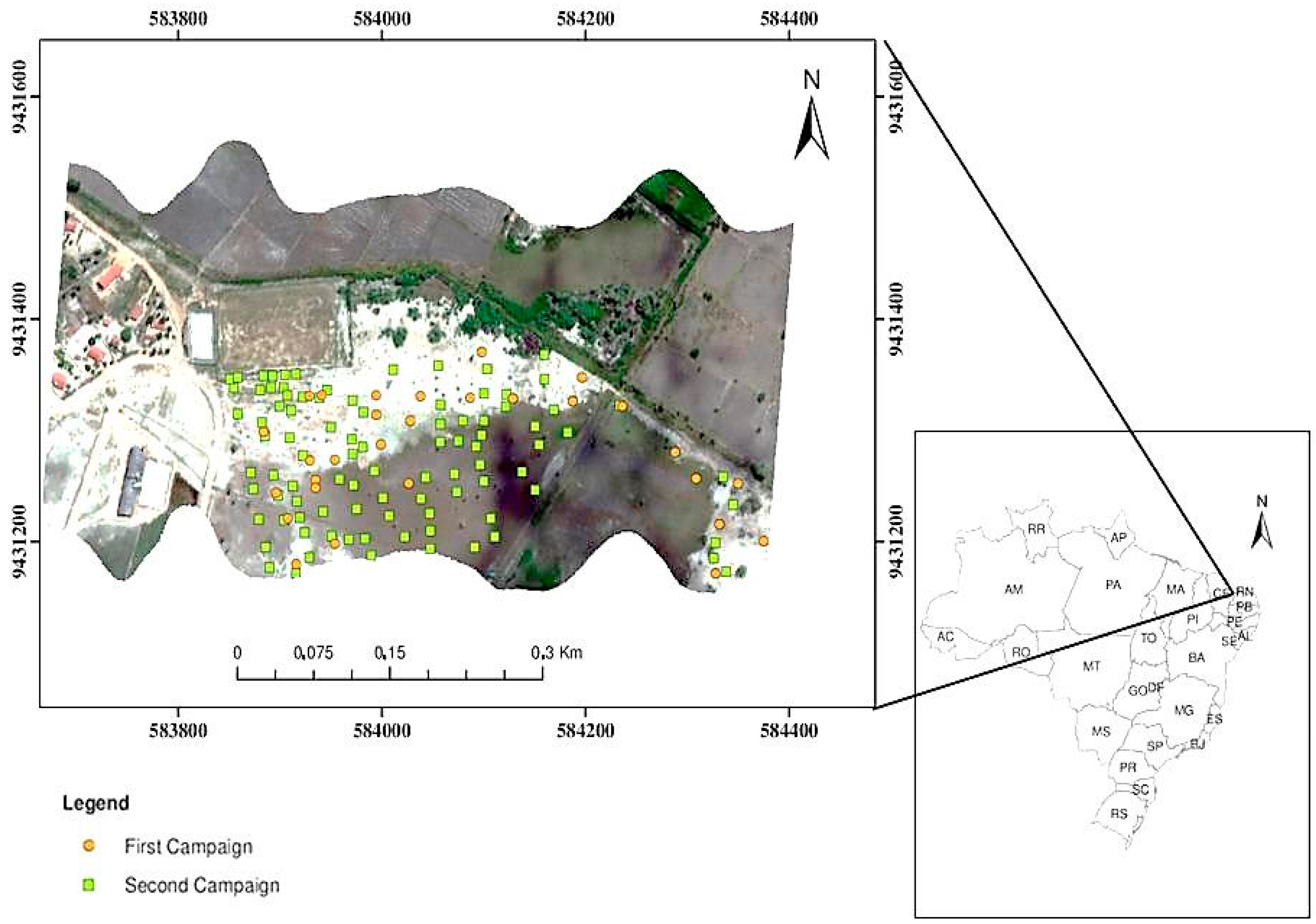
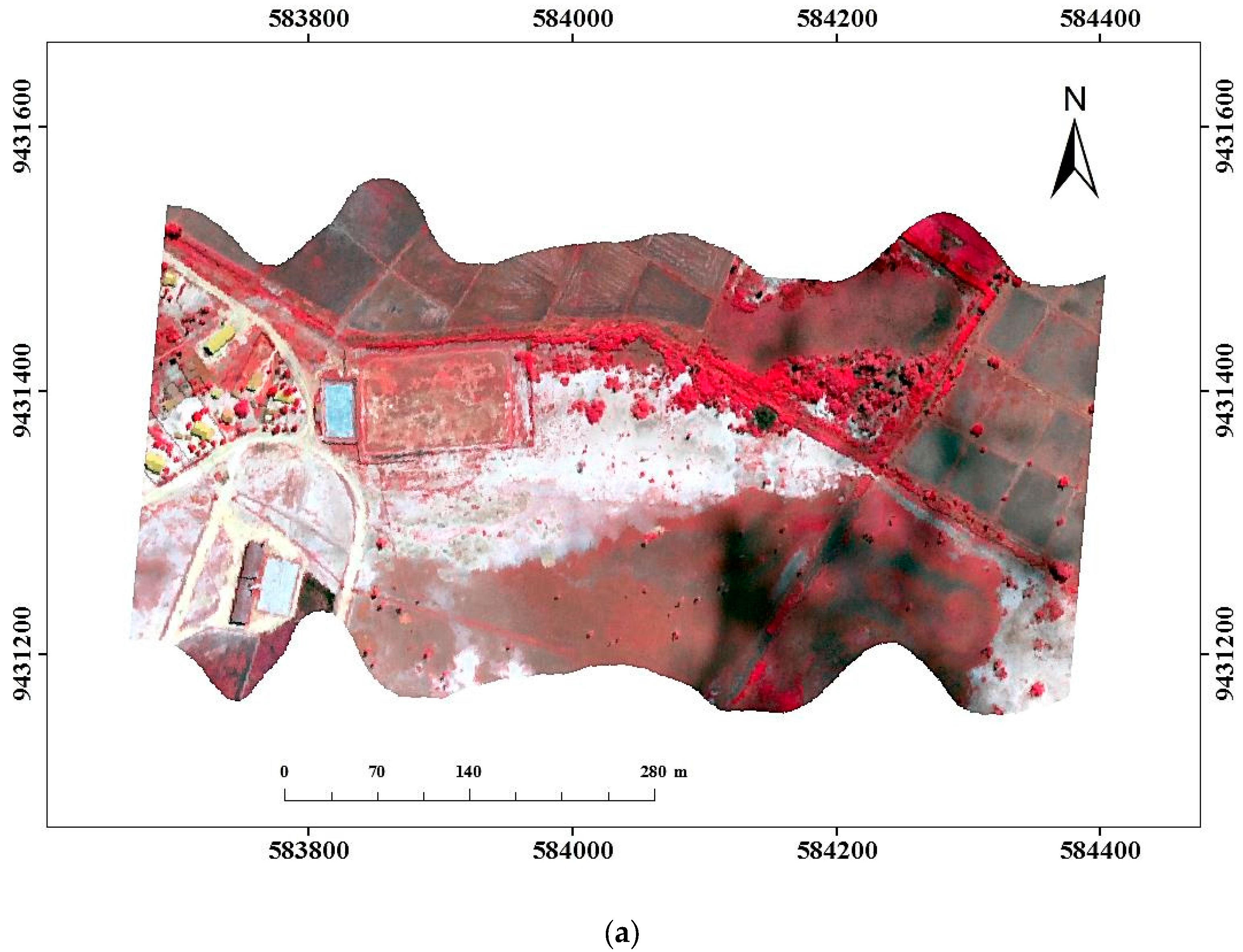
The Morada Nova Irrigation District, which has several problems of soil salinization associated with the cultivation of irrigated rice, was selected as the study area. The irrigated area is located in the towns of Morada Nova and Limoeiro do Norte, in the State of Ceará, in the Banabuiú sub-basin of the Lower Jaguaribe micro-region, 170 km from Fortaleza (Figure 1).

In the Morada Nova Irrigated Area, there is a predominance of two types of soil: Fluvic Neosols (75% of the study area) and Litholic Neosols (25% of the area) [19]. The first are alluvial soils, generally cultivated with rice for many years, which display many problems of salinization, while the latter are unsuitable for agriculture. According to Ferreyra and Silva [19], the mineralogical composition of these soils is a mixture, in which 2:1 minerals, both expansive (vermiculite and montmorillonite) and non-expansive (mica and illite), predominate in relation to kaolinite and quartz. According to the Köppen classification, the climate corresponds to BSW’h’ (very hot and semi-arid), with an average annual rainfall of less than 900 mm. Rainfall distribution is unimodal, with 80% of the total rain concentrated in the first four months of the year.

2.2. Field Data Collection

The study focused on the eastern part of the irrigated area (Figure 1). Soil samples were collected over agricultural fields previously cultivated with rice. Salinization problems were reported for most of these fields, affecting crop yield.

Two field campaigns were carried out to collect soil samples. In the first campaign (12 May 2015), 46 soil samples were collected from the surface horizon (0–10 cm). In the second campaign (31 August 2015), 107 topsoil samples were collected. The samples were taken to the laboratory, and then ground and sieved (2 mm) to reduce the effect of surface roughness.

2.3. EC and Spectral Reflectance Measurements

EC data were obtained in the laboratory using a bench conductivity meter with a range between 0 and 20 dS·m⁻¹. The EC was measured from a 1:1 dilution extract (soil sample: distilled water). The measurements were performed after 24 h of dilution.

To obtain spectral data in the laboratory, the FieldSpec Pro FR-3 spectrometer (Analytical Spectral Devices, Inc., Boulder, CO, USA) was used in a controlled environment (dark room). This equipment has a spectral resolution of three nm in the visible and near infrared region (VNIR = 350–1300 nm), and of 10 nm in the shortwave infrared (SWIR = 1300–2500 nm). At the nadir, the sensor was positioned at a distance of 7 cm from the soil sample to measure a circular area of 3 cm in diameter. The light source was a 250 W tungsten-halogen lamp with parabolic reflector and collimated beam along the target plane, and a zenith angle of 45°. To obtain the reflectance of the soil sample, white Spectralon of known reflectance was used as reference standard. Three readings were made by the spectrometer for the calculation of the mean reflectance with a sample rotation of 120° to reduce the influence of soil roughness and bidirectional effects on the spectral measurements.

2.4. Generation of the OLS, PLSR, MLP, and ELM Models with Laboratory Data

2.4.1. Model Calibration

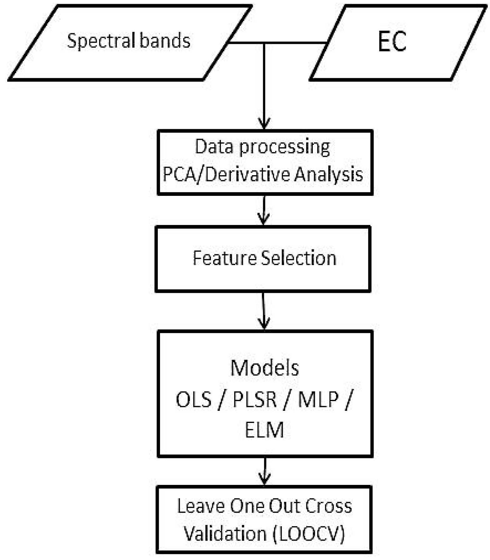
The methodology used to develop the models is presented in Figure 2. The first step consisted of model calibration or data processing. At this stage, laboratory reflectance data obtained with the FieldSpec Pro FR-3 were resampled to the 357 bands of the ProSpecTIR-VS airborne hyperspectral sensor. Earlier studies have shown that PCA can be useful in studies of soil salinity, since the first component is usually associated with the brightness (average reflectance) of the samples, which increases with salt concentration [20,21,22]. It was therefore decided that PCA should be applied to the laboratory data resampled to the bands of the ProSpecTIR-VS. As the first derivative can enhance spectral features associated with salts, derivative analysis was applied to the resampled reflectance data, preceded by the use of a moving average filter with a three-band window.

Due to the large number of attributes, both in the original data (reflectance) and in the transformed data (PCA and first derivative), the second step included feature selection from each data set. The forward feature selection process was used, where the selected attributes are initially unitary, and the remaining attributes are added according to an adjustment increment. The increment adopted was the adjusted coefficient of determination (adjusted R²). The stopping criteria for the algorithm were to obtain an adjusted R² greater than 95% and a maximum total of attributes equal to 25% of the sample size. This second criterion was adopted to avoid possible overfitting, thereby ensuring the generalization power of the model.

2.4.2. Model Validation

Model validation was performed using leave one out cross validation (LOOCV) (Figure 2). The parameters of the OLS, PLSR, MLP, and ELM models necessary for calibration and the resulting transformation matrices were obtained. The following parameters were used to evaluate the MLP neural network: five neurons in the hidden layer, randomly chosen weights, a learning rate of 95%, a logistic sigmoid activation function, and 5000 learning epochs. For the ELM model, the following parameters were used: five neurons in the hidden layer and a logistic sigmoid activation function.

2.5. Evaluation of the OLS, PLSR, MLP, and ELM Models with Laboratory Data

The evaluation of the four tested models was made according to the following statistical metrics: adjusted R², root mean square error (RMSE), the Pearson correlation coefficient (r), and the ratio of the performance to deviation (RPD). The coefficient of determination was calculated during the calibration stage. The other metrics were obtained during the validation stage.

As shown by Huang et al. [12], a large number of training samples are necessary to achieve the desired performance with the ELM model. Therefore, to optimize the total number of samples collected in the field, the technique of LOOCV was applied, where the separation of data into calibration and validation is repeated for a number of times equal to the total number of collected samples (n = 153), leaving out one sample. In each of the repetitions, the data set used for validation is unitary and new in relation to the other repetitions, a process that is repeated until all the collected samples have been used to validate the model. The results obtained with the validation metrics are equal to the average value of the results from the repetitions.

2.6. Model Application Using the ProSpecTIR-VS Hyperspectral Images

The best laboratory-calibrated model was inverted to the reflectance data obtained by the ProSpecTIR-SV airborne sensor. The image was acquired by the Fototerra Company on 23 May 2015. The sensor operates in 357 spectral bands located between 400 and 2500 nm, and spaced at intervals of 5 nm. The spatial resolution was 1 m, and the images were acquired at 1:00 p.m. (local time). During image acquisition, the agricultural fields were not under irrigation, which could affect the relationships between reflectance and soil salinity.

Radiance data measured by the ProSpecTIR-VS sensor were corrected for the effects of scattering and absorption by atmospheric gases and converted into surface reflectance using the ATCOR4. A rural tropical atmospheric model was adopted. The water vapor was calculated using the absorption bands located at 940 nm and 1130 nm. The images were corrected geometrically using data from the inertial navigation system of the aircraft.

To separate the pixels of exposed soil in the image from other scene components, the Normalized Difference Vegetation Index (NDVI) was calculated. Exposed soils generally exhibit NDVI values of less than 0.30 [23,24], a threshold that was tested and adopted in the present study. For the purposes of validating the laboratory-calibrated model applied to the image, EC data estimated for 32 pixels located in areas of exposed soil (NDVI < 0.30) in the image were plotted as a function of the EC values for the corresponding soil samples measured in the laboratory in the first campaign (12 May 2015). These pixels were selected independently from the training sample locations for model building.

2.7. Influence of Bandwidth and Band Positioning on Soil EC Estimates

To evaluate the performance of the four computational models as a function of the spectral resolution, we simulated two hyperspectral sensors and three multispectral instruments. The objective was to evaluate the influence of bandwidth and band positioning on the results. The selected hyperspectral instruments simulated from the laboratory data were the airborne ProSpecTIR-VS and the planned orbital Hyperspectral Infrared Imager (HyspIRI) with bandwidth of 5 nm and 10 nm, respectively, between 400 and 2500 nm. The multispectral sensors were simulated using their filter functions, including the RapidEye/REIS, High Resolution Geometric (HRG)/SPOT-5, and the Operational Land Imager (OLI)/Landsat-8)).

The RapidEye has five bands in the VNIR interval: 1 (blue; 440–510 nm), 2 (green; 520–590 nm), 3 (red; 630–685 nm), 4 (red edge; 690–730 nm), and 5 (NIR; 760–850 nm). The HRG has four bands in the VNIR/SWIR-1 spectral range: 1 (green; 500–590 nm), 2 (red; 610–680 nm), 3 (NIR; 780–890 nm), and 4 (SWIR-1; 1580–1750 nm). Finally, we simulated seven of the nine reflective bands of OLI: 1 (blue; 435–451 nm), 2 (blue; 452–512 nm), 3 (green; 533–590 nm), 4 (red; 636–673 nm), 5 (NIR; 851–879 nm), 6 (SWIR-1; 1566–1651 nm), and 7 (SWIR-2; 2107–22,294 nm).

Therefore, the simulation of ProSpecTIR-VS and HyspIRI, compared to the other sensors, represents the transition from narrowband to broadband sensors. On the other hand, the simulation from RapidEye to OLI represents the change in band positioning from the VNIR to the SWIR-1 and SWIR-2 spectral intervals.

Evaluation of the performance of the four models for the simulated sensors followed the protocol described before in Section 2.5.

3. Results

3.1. Spectral Reflectance of the Saline Soils and Feature Selection

Table 1. Descriptive statistics of the electrical conductivity (EC) of the soils and autocorrelation measurement between the samples.

Mean (dS·m−1)	Maximum (dS·m−1)	Minimum (dS·m−1)	Standard Deviation (dS·m−1)	Coefficient of Variation (%)	n	Moran’s Autocorrelation Index
7.82	19.90	0.90	4.67	21.83	153	0.261

shows the descriptive statistics of the EC that had a mean value of 7.82 dS·m⁻¹ and a standard deviation of 4.67 dS·m⁻¹. The Moran’s index indicated the absence of autocorrelation between the samples collected in the field. Figure 3 shows reflectance spectra representative of soils with increased levels of salinization or EC. Reflectance increased at the different wavelengths with soil salinization, expressed by different values of soil EC. When compared with other salts (e.g., CaCl₂ and MgCl₂), the effect of NaCl is to increase soil reflectance in the VNIR and SWIR [25]. The salt also produces absorption bands at 1450 nm and 1950 nm, related to fluid inclusion, absorbed water, or even soil moisture. In the spectra here, the absorption bands became deeper as soil salinity increased (Figure 3). The absorption band centered at 2200 nm, typically associated with the hydroxyl of clay minerals, was also detected in the spectra of soils from the study area.

When spectroradiometric data from the laboratory were simulated for the 357 bands of the ProSpecTIR-VS and subjected to the feature selection algorithm for estimating soil EC, the best results were obtained with the reflectance of three bands located at 395, 1642, and 1717 nm (adjusted R² = 0.953) (

Table 2. Feature selection between transformed spectroradiometric data (derivative analysis and principal component analysis - PCA) and non-transformed data (reflectance), after resampling to the 357 bands of the ProSpecTIR-VS hyperspectral sensor.

Data Transformation	n	Selected Feature	Adjusted R2
Reflectance (original)	3	395, 1642, 1717 nm	0.953
Derivative analysis	38	409, 596, 629, 657, 700, 724, 729, 738, 743, 772, 826, 994, 1133, 1140, 1171, 1196, 1222, 1234, 1241, 1398, 1410, 1542, 1573, 1817, 1829, 1867, 1904, 1910, 2016, 2173, 2191, 2229, 2279, 2304, 2348, 2354, 2379, 2429 nm	0.619
PCA	6	1, 2, 3, 5, 6, 10	0.957

). When PCA was applied to the reflectance data, the algorithm selected six principal components having an approximately equal value for the adjusted R² (0.957). On the other hand, band selection after derivative analysis was not effective, producing low values for the adjusted R² (0.619) even after the selection of a relatively large number of bands (38 bands in Table 2).

The relationships between soil EC and the reflectance of the ProSpecTIR-VS band located at 1642 nm (Figure 4a) and for the first principal component (PC1) (Figure 4b), were not completely linear, especially for EC values below 5 dS·m⁻¹. Assuming a linear relationship, the greatest value for R² was obtained with PC1 (R² = 0.895) when compared to the reflectance at 1642 nm (R² = 0.777).

3.2. Performance Evaluation of the OLS, PLSR, MLP, and ELM Models

The performance of the linear models and ELM to estimate soil EC with reflectance and PCA was better than that of the MLP. Compared to MLP, the OLS, PLSR, and ELM models presented larger values of r and RPD, and lower values of RMSE (

Table 3. Performance of Ordinary Least Squares (OLS), Partial Least Squares Regression (PLSR), Multilayer Perceptron (MLP), and Extreme Learning Machine (ELM) in estimating soil electrical conductivity (EC) using transformed and non-transformed reflectance data.

Transformation	Model	Mean Error (dS·m−1)	RMSE (dS·m−1)	r	RPD
Reflectance (no transformation)	OLS	0.001064	0.109996	0.9643	46.72
	PLSR	0.000982	0.099936	0.9698	46.73
	MLP	−0.008723	0.120006	0.7724	35.64
	ELM	−0.001077	0.110011	0.9585	44.55
Derivative Analysis	OLS	0.026216	3.744000	0.8168	1.25
	PLSR	−0.016673	3.732100	0.8274	1.26
	MLP	0.092369	4.159821	0.2644	1.12
	ELM	0.047595	3.840164	0.6237	1.22
PCA	OLS	−0.001354	0.140012	0.9735	32.04
	PLSR	−0.001278	0.130016	0.9758	32.05
	MLP	0.010228	0.140714	0.8579	29.44
	ELM	−0.001370	0.139988	0.9632	32.71

RMSE = root mean square error; r = Pearson’s correlation coefficient; RPD = ratio of the performance to deviation.

). None of the three models performed well with the first derivative data of the reflectance spectra, with RPD values equal to or less than 1.25, indicating unreliable predictive models.

When the values measured for EC were plotted as a function of the values estimated by the PLSR model using reflectance data (bands at 395, 1642, and 1717 nm), an RMSE value of 0.7705 dS·m⁻¹ was obtained (Figure 5).

3.3. Laboratory-Calibrated PLSR Model Applied to Estimate Soil EC in the ProSpecTIR-VS Image

Considering all of the metrics from Table 3, the best model was the PLSR with the reflectance (ρ) of the simulated bands of the ProSpecTIR-VS sensor located at 395, 1642, and 1717 nm (Equation (1)):

$$\mathrm{EC}=-3.75+32.3412{\mathsf{\rho }}_{395\mathrm{nm}}+96.5541{\mathsf{\rho }}_{1642\mathrm{nm}}-300.4515{\mathsf{\rho }}_{1717\mathrm{nm}}$$

(1)

When compared to data measured in the laboratory, the values for EC estimated by the PLSR model (Equation (1)) in the ProSpecTIR-VS scene, for 32 pixels equivalent to sample collection points in areas of exposed soil (NDVI < 0.30), produced an RMSE of 1.22 dS·m⁻¹ (Figure 6).

Figure 7a shows a false color composite of the study area, obtained with the bands of the ProSpecTIR-VS sensor located at 860, 648, and 549 nm displayed in red, green, and blue, respectively. Figure 7b shows EC values estimated with the PLSR model (Equation (1)) for the areas of exposed soils (NDVI less than 0.3). In Figure 7a, the arboreal vegetation and agricultural crops appear in reddish tones, while the areas of exposed soil appear whitish.

3.4. Influence of Bandwidth and Band Positioning on Soil EC Estimates

When the feature selection algorithm was applied over the data, a subset of three bands was selected for the simulated hyperspectral sensors (ProSpecTIR-VS and HyspIRI) and all the bands were chosen for the simulated multispectral instruments (RapidEye/REIS, HRG/SPOT-5 and OLI/Landsat-8) (

Table 4. Feature selection for bands of the simulated hyperspectral and multispectral sensors using the laboratory reflectance data.

Data Transformation	n	Selected Feature	Adjusted R2
ProSpecTIR-VS	3	395, 1642, 1717 nm	0.953
HyspIRI	3	390, 1200, 1630 nm	0.950
RapidEye/REIS	5	All bands	0.153
HRG/SPOT-5	4	All bands	0.456
OLI/Landsat-8	6	All bands	0.553

). The performance of the narrowband sensors (ProSpecTIR-VS and HyspIRI) was better than the broadband instruments, as indicated by the comparatively higher adjusted R² values (Table 4).

For the four studied computational models, the results improved with increased spectral resolution from the multispectral sensors to the hyperspectral instruments, as indicated by lower RMSE values and by larger r and RPD values observed for ProSpecTIR-VS and HyspIRI (

Table 5. Performance of the Ordinary Least Squares (OLS), Partial Least Squares Regression (PLSR), Multilayer Perceptron (MLP), and Extreme Learning Machine (ELM) models to estimate soil EC as a function of the spectral resolution simulation of different hyperspectral and multispectral sensors.

Simulated Sensor	Model	Mean Error	RMSE	R	RPD
		(dS·m−1)	(dS·m−1)
ProSpecTIR-VS	OLS	0.001064	0.109996	0.9647	46.72
	PLSR	0.000982	0.099936	0.9698	46.73
	MLP	−0.008723	0.120006	0.7724	35.64
	ELM	−0.001077	0.110011	0.9585	44.55
HyspIRI	OLS	−0.001078	0.110022	0.9596	46.65
	PLSR	−0.000914	0.099979	0.9685	47.71
	MLP	−0.007997	0.110012	0.8641	40.62
	ELM	0.001175	0.110018	0.9626	44.98
RapidEye/REIS	OLS	0.044688	4.619802	0.3127	1.01
	PLSR	0.043199	4.396226	0.3435	1.06
	MLP	−0.073114	5.133092	0.2901	0.90
	ELM	0.034349	4.530097	0.3247	1.03
HRG/SPOT-5	OLS	0.020606	2.130286	0.5112	1.75
	PLSR	0.019950	2.029891	0.5354	1.84
	MLP	−0.082261	2.369872	0.4632	1.56
	ELM	0.040459	2.089888	0.5242	1.78
OLI/Landsat-8	OLS	0.024781	2.561905	0.6216	2.10
	PLSR	−0.013974	2.439819	0.6529	2.21
	MLP	0.026442	2.840107	0.5468	1.87
	ELM	−0.024571	2.509813	0.6273	2.14

RMSE = root mean square error; r = Pearson correlation coefficient; RPD = ratio of the performance to deviation.

). From the set of simulated multispectral sensors, the RPD values increased from the RapidEye to the HRG and OLI, which indicated the importance of the SWIR-1 and SWIR-2 bands on soil EC estimates (Table 5).

Overall, the performance of the PLSR model was better than the other models to estimate soil EC for both simulated multispectral and hyperspectral sensors, as shown by the RPD values in the last column of Table 5.

4. Discussion

We studied the performance of four computational models with different spectral attributes as a function of the spectral resolution of hyperspectral and multispectral sensors, and used the best laboratory-calibrated model to estimate soil EC on a per-pixel basis in a hyperspectral image acquired by the airborne ProSpecTIR-VS instrument. Our findings showed that the OLS, PLSR, and ELM models performed better than the MLP model in estimating soil EC with the metrics related to soil brightness having greater predictive power than the metrics related to spectral features. The laboratory models were transferable to the aircraft level of data acquisition with their performance to estimate soil EC being better for simulated narrowband sensors (ProSpecTIR-VS and HyspIRI) than for simulated broadband instruments (RapidEye, HRG, and OLI).

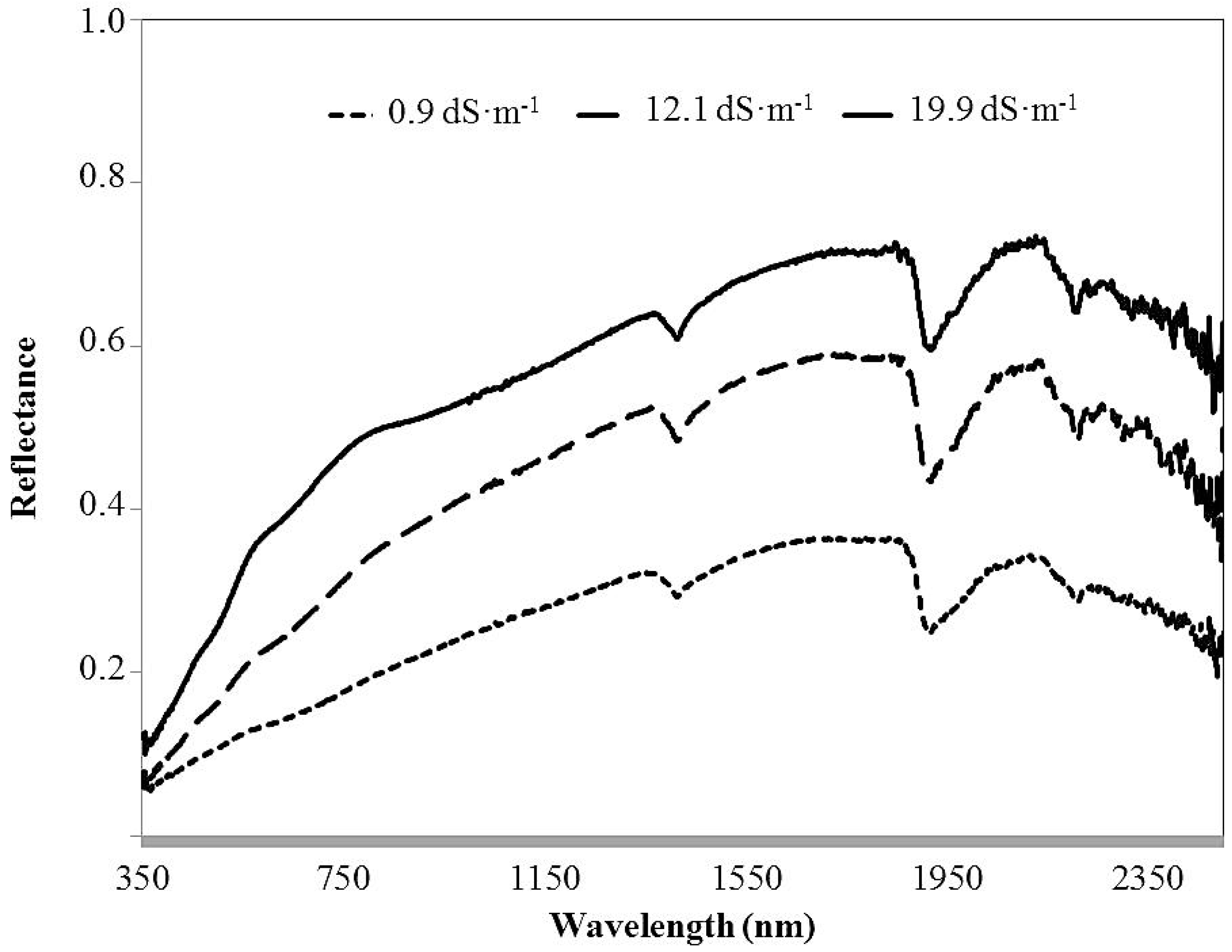
In our study, soil brightness was mostly controlled by variations in soil salinization. In contrast to the other salts (e.g., MgCl₂ and CaCl₂), the effect of NaCl is to increase soil brightness, as also observed in other studies [25]. In addition, NaCl produces also absorption bands at 1450 and 1950 nm related to fluid inclusions or absorbed water [26]. Unfortunately, these features in pixel spectra are coincident with strong water vapor absorptions that cannot be used in the data analysis even after atmospheric correction. Overall, our results are in agreement with those obtained by Moreira et al. [22], who observed a positive correlation between soil brightness and soil salinization, as expressed by increasing values of EC. Such correlation is not observed for all the salts and is typical of the predominance of NaCl. For instance, when treating the soils of the study area with increasing levels of salinization in the laboratory, Moreira et al. [27] observed an increase in brightness for NaCl and a decrease in brightness for MgCl₂ and CaCl₂ with increased salt concentration.

Compared to the absorption bands, which were indirectly represented by the calculation of first-order derivative spectra, our feature selection procedure confirmed that soil brightness, expressed by the reflectance of selected bands and PCA scores, was more sensitive to changes in salt concentration. When studying different computational models to estimate soil EC, Mashimbye et al. 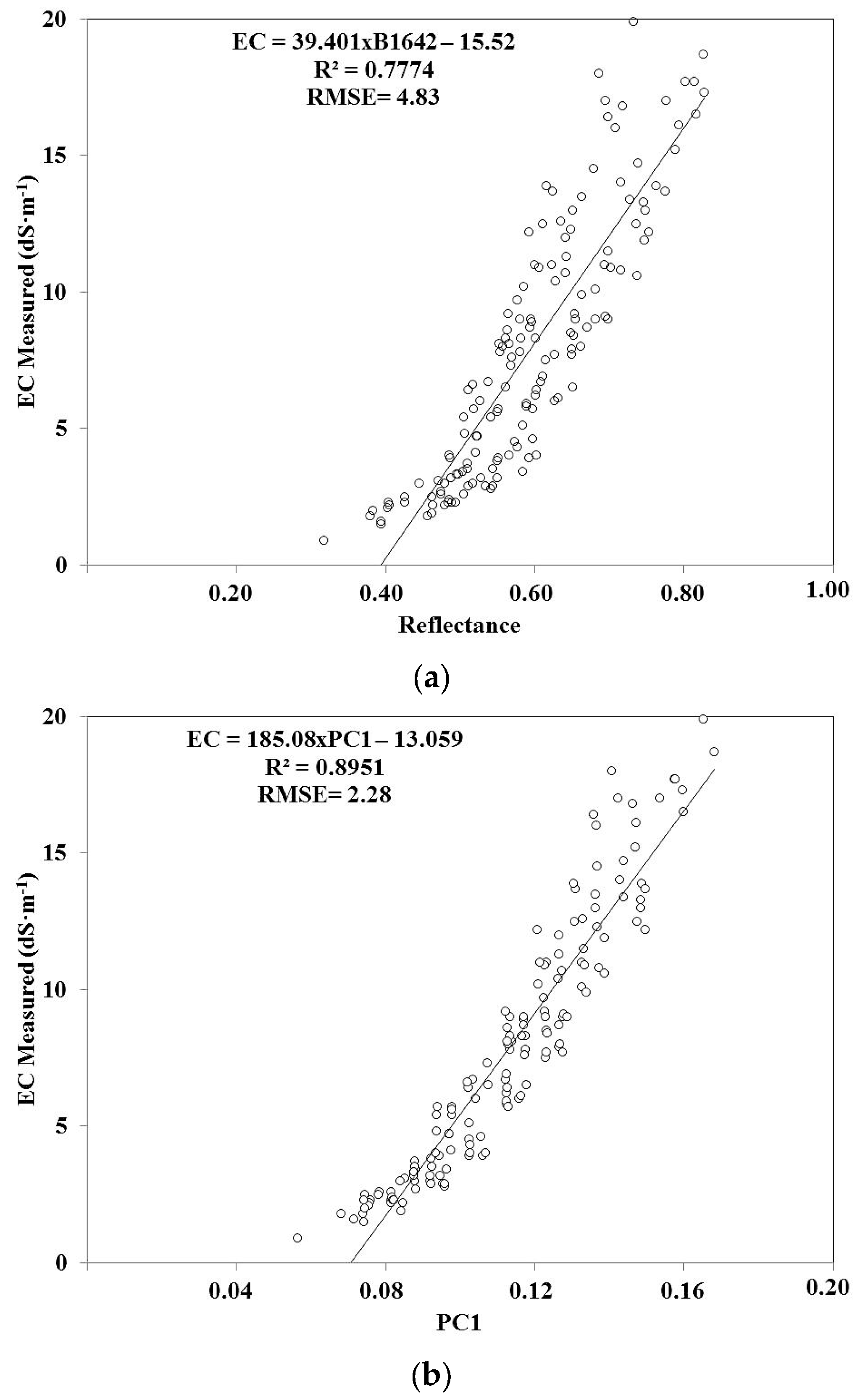[5] obtained a lower adjusted R² for the first-order derivative than for the original reflectance, which was in agreement with the current results. In the literature, soil brightness is generally related to the first principal component [22]. Brightness corresponds approximately to the mean reflectance calculated between 400 and 2500 nm. Our results confirmed PC1 as a proxy of soil brightness because its eigenvector loadings were approximately similar for the 357 simulated VNIR-SWIR bands of the ProSpecTIR-VS. As a result, PC1 was highly correlated with the average reflectance calculated between 400 and 2500 nm (r = +0.87), as also observed by Moreira et al. [22]. That was the reason that PC1 and the reflectance of three bands placed in this interval were selected as the best attributes for the computational models.

In order to estimate soil EC using remote sensing, most studies indicated a superior performance of the linear models compared to the non-linear models [11]. The best performance of the PLSR model to estimate soil EC in our study area was also consistent with the work by Kumar et al. [4], when using the reflectance of Hyperion bands as input variables for the model. However, the modified approach proposed by Huang et al. [12] in the ELM model produced results in northeastern Brazil comparable in performance with the PLSR, as indicated by the different statistical metrics (r, RMSE, and RPD). It is well known that neural networks models benefit from a large number of samples [12]. Therefore, the performance of the neural algorithms may be underestimated here because they have an accuracy that is generally affected by the number of training samples, which is relatively small in our work. Another factor that can affect the reliability of the models for detecting soil salinization is the spatial dependence of the soil samples collected in the field. In our study, we checked for spatial autocorrelation between the samples using the Moran’s Index with the value of 0.261 indicating the absence of spatial autocorrelation.

When evaluating the predictive ability of linear models to estimate soil EC using PCA, derivative analysis, and band ratioing, Mashimbye et al. [5] observed that the best results were associated with the PCA set of laboratory attributes. In agreement with our findings, Kobayashi et al. [8] noted that the predictive power of the reflectance of bands positioned between 1970 and 2130 nm was higher than the use of the first-order derivative. Because soil brightness is probably the most sensitive attribute to soil salinization in these studies [5,8,11], techniques to quantify absorption band parameters (e.g., derivative analysis and continuum removal) will not be effective to estimate soil EC in areas where NaCl is the predominant salt.

Our results from sensor simulation were in agreement with a recent study by Castaldi et al. [28]. When evaluating the potential of the current and forthcoming multispectral and hyperspectral sensors to estimate physico-chemical attributes of soils from Europe using PLSR, Castaldi et al. [29] found large RPD values for simulated hyperspectral instruments than for multispectral sensors. Although brightness was the best indicator of soil salinization in our study area, our results with the simulation of RapidEye, HRG, and OLI showed the importance of the SWIR-1 and SWIR-2 spectral information to compose this attribute, or if the choice is to use selected bands to estimate soil EC.

Some constraints should be analyzed with care during the transition from the laboratory to the airborne level of data acquisition. First, the models were developed under a controlled environment and the soils were dried and sieved. As a result, soil structure was not preserved, which is an important factor for salinization. Second, soil moisture in the field reduces the reflectance, from the VNIR to SWIR, which introduces uncertainties on the EC estimates of the pixels, especially during the rainy season. Finally, because brightness or the reflectance of selected bands of the airborne ProSpecTIR-VS were the most sensitive attributes to detect soil salinization in the study area, care is necessary during the planning of the flightlines. These attributes do not normalize bidirectional effects associated with variations in solar zenith angle (SZA) and relative azimuth angle (RAA) between the sensor and the sun. If several flightlines are programmed for a given region, the best strategy is to fix the period of data acquisition (time and date) and the direction of the lines (e.g., NNE/SSW) to reduce bidirectional effects on reflectance and EC estimates over the images. For differently oriented flightlines, an alternative is to look for the best band-ratio index to detect soil salinization and normalize the bidirectional effects.

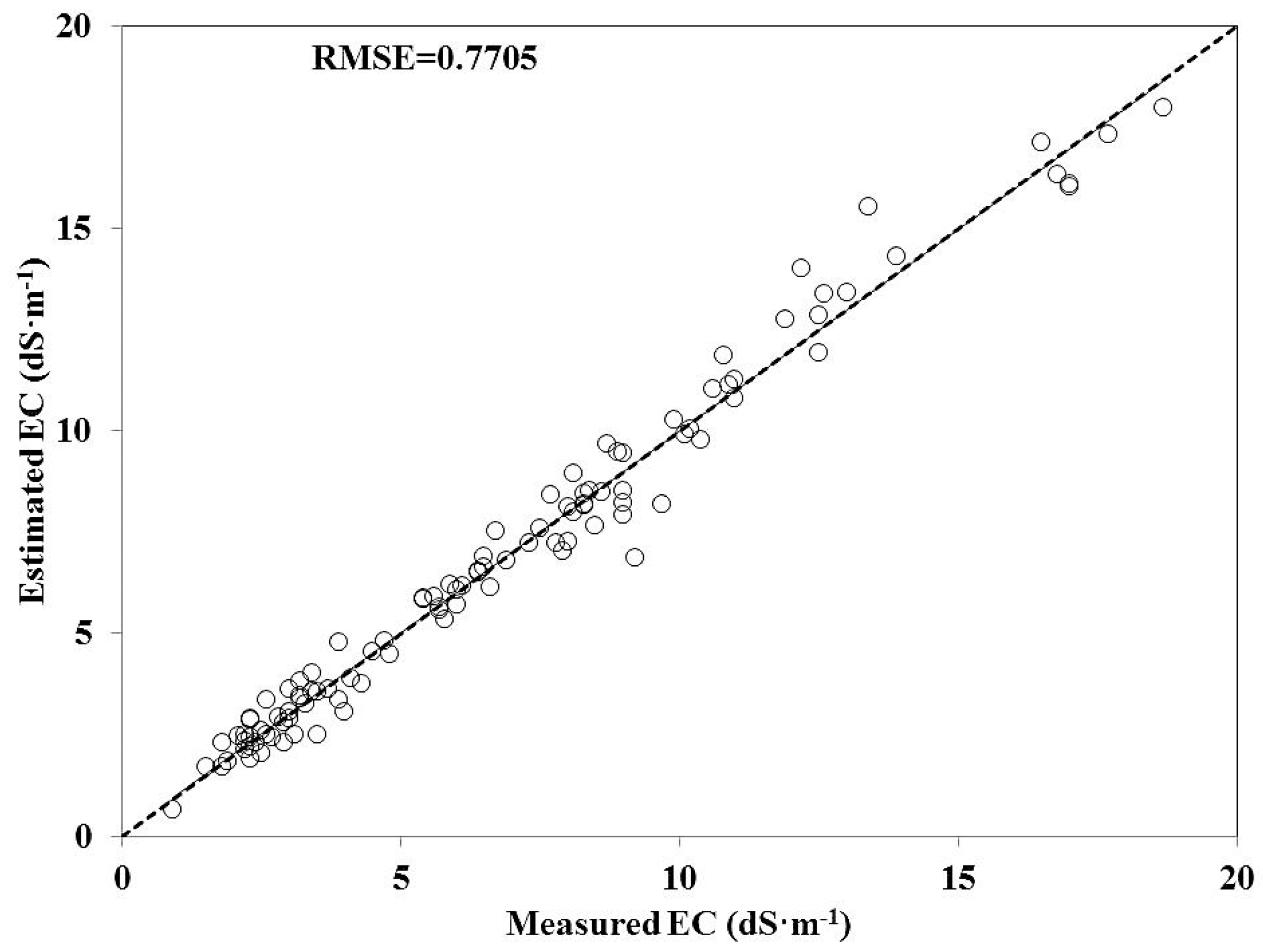
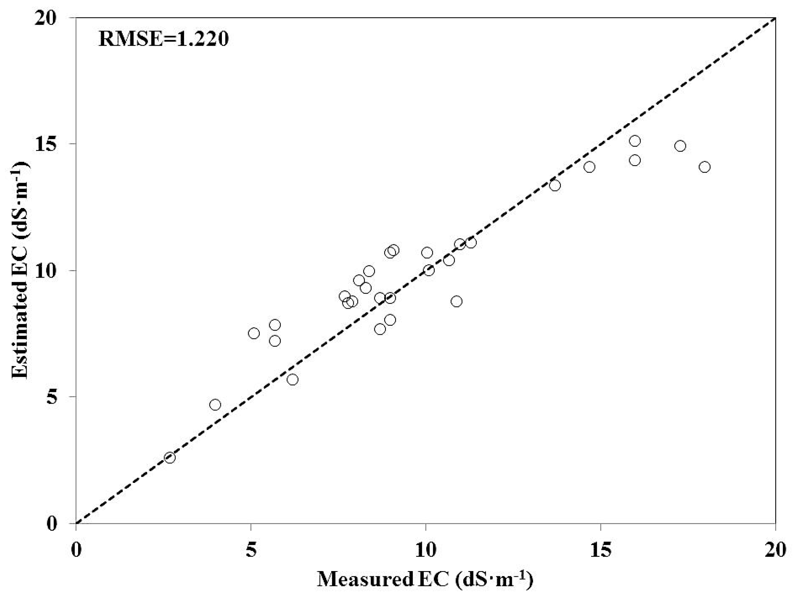
When the PLSR-calibrated model using reflectance of selected bands was applied to the ProSpecTIR-VS image, the RMSE from the validation set of samples was higher (1.22 dS·m⁻¹) than that obtained with soil samples under controlled laboratory conditions (RMSE = 0.77 dS·m⁻¹). This result was expected because the transition from the laboratory to the airborne level of data acquisition produces a greater influence of other factors over the EC estimates such as spectral mixture and signal-to-noise (SNR). Despite these factors, the RPD was 2.21, which still indicates the adequacy of the predictive ability of the PLSR model. The reduction in model performance with the scaling up of observations from laboratory to satellite was also observed by Zhang et al. [27], after modeling Ca²⁺ using Hyperion/EO-1 data in a land degradation area in China. They highlighted the poor SNR of Hyperion as one of the factors that affected the quality of the estimates.

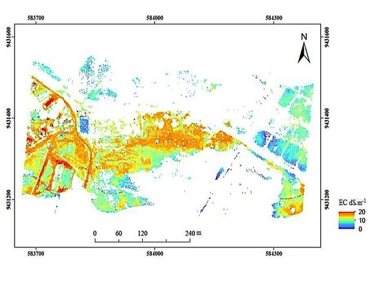
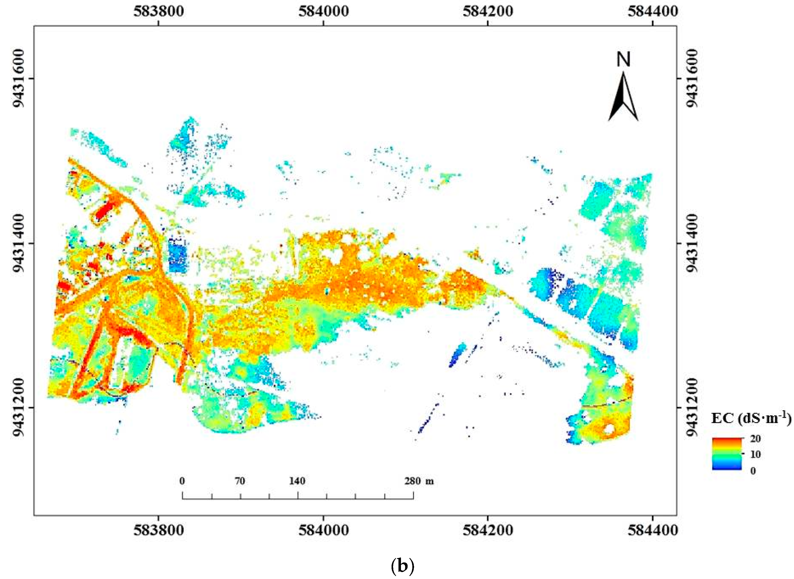
Our soil salinization map (Figure 7) detected greater amounts of saline soils in the central portion of the study area with EC ranging from 10 to 20 dS·m⁻¹. These values are generally the result of inadequate irrigation and poor drainage of soils, which affect crop yield (e.g., rice) and cause subsequent land abandonment [22]. Our results have shown the importance of testing different models to estimate soil EC using hyperspectral data. They can contribute to data analysis of the upcoming orbital hyperspectral missions such as the EnMAP, planned for 2019 [10], and the HyspIRI. The HyspIRI has been proposed to obtain high spectral resolution data (380–2500 nm) over large areas with 30 m spatial resolution and 145 km swath width [29].

5. Conclusions

We investigated the performance of four computational models (OLS, PLSR, ELM, and MLP) with different attributes (reflectance, PCA scores, and first-order derivative), as a function of the spectral resolution of simulated hyperspectral and multispectral sensors. In addition, we used the best laboratory-calibrated model to estimate soil EC to aircraft level in a hyperspectral image obtained by the ProSpecTIR-VS airborne sensor. From the four specific objectives defined in this study, the following conclusions were obtained:

(1)

The OLS, PLSR, and ELM models performed better than the MLP model in estimating EC in saline soils using spectroradiometric laboratory data. They presented larger adjusted R², r, and RPD, and lower RMSE than the MLP model;

(2)

From the spectral attributes tested for estimating soil EC, and after feature selection, the metrics related to soil brightness (reflectance and principal components) had greater predictive power than the metrics related to spectral features (first-order derivative), irrespective of the type of model used;

(3)

The laboratory models were transferable to the aircraft level of data acquisition (ProSpecTIR-VS hyperspectral sensor), continuing to perform well in the pixel-by-pixel estimation of the exposed soil EC in the image. The greatest salinity levels were detected in exposed soils (NDVI < 0.30) from the central part of the study area, with EC estimates ranging from 10 to 20 dS·m⁻¹;

(4)

Finally, for all the models and simulated sensors, the performance of the narrowband sensors (ProSpecTIR-VS and HyspIRI) to estimate soil EC was better than the performance of the broadband instruments (RapidEye, HRG, and OLI). Within the set of multispectral sensors, the RPD values increased from the RapidEye to the HRG and OLI, which indicated the importance of the SWIR-1 and SWIR-2 bands to estimate soil EC.